OSMOTIC POWER FOR REMOTE COMMUNITIES IN QUEBEC. Jonathan Maisonneuve. A Thesis. In the Department. Electrical and Computer Engineering

Transcription

1 OSMOTIC POWER FOR REMOTE COMMUNITIES IN QUEBEC Jonathan Maisonneuve A Thesis In the Department of Electrical and Computer Engineering Presented in Partial Fulfillment of the Requirements For the Degree of Doctor of Philosophy (Electrical and Computer Engineering) at Concordia University Montreal, Quebec, Canada August 215 Jonathan Maisonneuve, 215

2 This is to certify that the thesis prepared CONCORDIA UNIVERSITY SCHOOL OF GRADUATE STUDIES By: Entitled: Jonathan Maisonneuve Osmotic Power for Remote Communities in Quebec and submitted in partial fulfillment of the requirements for the degree of Doctor of Philosophy (Electrical and Computer Engineering) complies with the regulations of the University and meets the accepted standards with respect to originality and quality. Signed by the final examining committee: Dr. D. Dysart-Gale Dr. M. El-Hawary Dr. A. Athienitis Dr. L. A. C. Lopes Dr. H. Zad Dr. P. Pillay Chair External Examiner External to Program Examiner Examiner Thesis Supervisor Approved by: Dr. A. R. Sebak, Graduate Program Director August 12, 215 Dr. A. Asif, Dean Faculty of Engineering and Computer Science ii

3 ABSTRACT Osmotic Power for Remote Communities in Quebec Jonathan Maisonneuve, Ph.D. Concordia University, 215 This work investigates the process of pressure retarded osmosis (PRO) for salinity gradient energy conversion in power production applications. A mathematical model of the PRO process is developed with consideration for non-ideal effects including internal concentration polarization, external concentration polarization, and spatial variations that are caused by mass transfer and by pressure drop along the length of the membrane. A mathematical model of the osmotic power plant is also developed with consideration for pre-filtration and pick-up head, and for mechanical and electrical equipment efficiencies. A distinction is made between the gross power developed by the PRO process, and the net power available to the grid after parasitic loads are accounted for. This distinction leads to observation of a trade-off that exists between the different non-ideal effects. A method is developed for adjusting operating conditions in order to minimize the overall impact of non-ideal effects and to achieve maximum net power. Important improvements in net power densities are realized as compared to results obtained when general rules of thumb are used for operating conditions. The mathematical model is validated by experimental investigation of PRO at the bench-scale. It is found that test conditions generally used in the literature may not be appropriate for power production applications. Test conditions which strike a balance between pressure drop and other non-ideal effects may provide more realistic results. iii

4 An analog electric circuit is developed for a simplified PRO process and osmotic power plant. The analog circuit is used to develop strategies for controlling operating conditions of the system, including by control of the load and by control of a flush valve. Both of these provide satisfactory tracking of the desired operating conditions and can also be used for tracking the maximum power point. The proposed strategies respond quickly to changes in source and load. The osmotic power potential is evaluated for remote micro-grids in Quebec. The osmotic power potential of selected rivers is calculated and compared against peak power demand of nearby communities. In each case, only a small portion of river flow is needed to satisfy the peak power demand of the micro-grids. This suggests that osmotic power can serve as a reliable source of electricity in such applications. An osmotic power plant prototype is designed for Quebec and its potential for power production in remote communities is evaluated. iv

5 ACKNOWLEDGEMENTS I would like to sincerely thank my supervisor Dr. Pragasen Pillay for his constant guidance and trusted direction throughout my Ph.D studies. I hope to emulate his honesty, integrity and wisdom throughout my career and beyond. I would like to thank Dr. Claude B. Laflamme from Hydro-Québec for his close collaboration. It was a pleasure to work with such a passionate researcher and interesting individual. I would also like to thank Mr. Guillaume Clairet from H 2 O Innovation and Dr. Catherine Mulligan from Concordia University for their many contributions to the Osmotic Power (OSMOP) research project. Many thanks to all of the professors and colleagues in the Power Electronics and Energy Research (PEER) group for their help and insights. It is a great privilege to have been part of such a world-class research group. I would like to express my deepest gratitude to my parents for their unconditional support throughout my entire life, to my beloved wife Ariane Avril, for her emotional support and continuous encouragement, and to my two children Eva and Henri. This research work was done as part of the NSERC/Hydro-Québec Industrial Research Chair entitled Design and Performance of Special Electrical Machines. It was also supported in part by the Fonds de Recherche du Québec - Nature et Technologies, and in part by Mitacs. v

6 TABLE OF CONTENTS 1. Introduction Background Objectives Thesis Outline Mathematical Model of Pressure Retarded Osmosis Power System Introduction Osmotically Driven Membrane Processes Water and Salt Permeate Gross PRO Power Concentration Polarization Variations along the Length of the Membrane Osmotic Power Plants Summary Experimental Investigation of Pressure Retarded Osmosis for Renewable Power Applications vi

7 3.1. Introduction Experimental Set-Up Membrane Characterization Gross PRO Power Density Net PRO Power Density Summary Analog Electric Circuit Model for Pressure Retarded Osmosis Introduction Water and Salt Flux across a Semi-Permeable Membrane Concentration Polarization Spatial Variations Osmotic Power System Control of Operating Conditions Maximum Power Point Tracking Summary Osmotic Power for Remote Communities in Quebec vii

8 5.1. Introduction Micro-Grids in Quebec Freshwater and Seawater Resources in Remote Regions of Quebec Power Potential of Selected Rivers Osmotic Power Plant Prototype for Quebec Summary Conclusions and Recommendations Conclusions Proposed Future Research Contributions viii

9 LIST OF FIGURES Figure 1. History of experimentally obtained power densities by PRO process with different draw solutions, modified from [1]... 7 Figure 2. Osmotically driven membrane processes: (a) forward osmosis (FO), (b) pressure retarded osmosis (PRO), (c) osmotic equilibrium (OE), and (d) reverse osmosis (RO)... 9 Figure 3. Water permeate flux across a semi-permeable membrane as a function of hydraulic pressure difference (normalized over the osmotic pressure difference)... 1 Figure 4. Water and salt flux across a short section of hollow fiber membrane Figure 5. Gross PRO power density as a function of hydraulic pressure difference (normalized over the osmotic pressure difference), where the theoretical maximum power is obtained when ΔP = ΔΓ m / Figure 6. Concentration profile across a semi-permeable membrane due to polarization 16 Figure 7. Model for solving polarization equation and determining power density Figure 8. Effective concentration difference, water permeate flux, and gross PRO power density as functions of hydraulic pressure difference for small scale samples of membranes ix

10 Figure 9. Gross PRO power density as a function of hydraulic pressure difference for small scale samples of membranes 1-4 when structure parameter is reduced to S = 349 μm Figure 1. Variation in flow rate and concentration on the (a) feed side and (b) draw side of the membrane Figure 11. Variation in flow rates, concentrations and hydraulic pressures along the length of the membrane Figure 12. Model for solving polarization equation and considering spatial variations along the length of membrane Figure 13. Single hollow fiber membrane module Figure 14. Spatial variation of bulk concentration c b, cross-flow velocity u, effective concentration difference, water permeate flux and gross PRO power density along the length of commercial scale membranes 3 (with S = 349 μm) and 4, when hydraulic pressure difference = bar Figure 15. Power density as a function of hydraulic pressure difference at the inlet and outlet of commercial length hollow fiber membrane 3 (with structure parameter adjusted to S = 349 μm) and membrane Figure 16. Power flow during PRO process x

11 Figure 17. Schematic for an osmotic power plant showing flow rates and hydraulic pressures throughout the system Figure 18. Power flow in osmotic power plant Figure 19. Model for osmotic power plant Figure 2. Simulated water permeate flux and gross PRO power density as compared to experimental results published by [36] using the following feed and draw concentrations (g/l): (a) and 35, (b) 2.5 and 35, (c) 5 and 35, (d) and 6, (e) 2.5 and 6, (f) 5 and Figure 21. Performance of osmotic power plant operated with inlet velocities u F (x = ) = u D (x = ) =.133 m/s and given the other conditions from Table Figure 22. The impact of varying inlet velocities u F (x = ) = u D (x = ) on (a) effective concentration differences (b) pressure losses and (c) net electric power density, when ΔP (x = ) = bar and given the other conditions from Table Figure 23. Best operating velocities and hydraulic pressure difference for the osmotic power plant described in Table Figure 24. Best operating velocities and hydraulic pressure difference for an osmotic power plant with membrane parameters A = m 3 /Pa s m 2, B = m 3 /s m 2 and S = m and with other conditions from Table Figure 25. PRO bench unit in the Hydro-Québec laboratory (Shawinigan, QC) xi

12 Figure 26. Custom cell for housing membrane samples, with length L = 25 mm, width w = 35 mm, and channel height on both sides of the membrane h = 1.2 mm Figure 27. Characteristic membrane parameters A, B, and S determined under test conditions from Table 6; box plot analysis shows the median (middle red line), 25 percentile (bottom of blue box), 75 percentile (top of blue box), range of data (extended black lines), and outliers (red cross) Figure 28. PRO performance under test conditions from Table 7, where experimental results (red points) and simulation results (blue lines) are shown for water permeate flux and gross PRO power density as functions of hydraulic pressure difference Figure 29. PRO performance under test conditions from Table 9, where experimental results (red points) and simulation results (blue lines) are shown for water permeate flux, gross PRO power density, feed side pressure drop, and net PRO power density, as functions of hydraulic pressure difference Figure 3. Effective height of the feed side channel under membrane distortion caused by applied hydraulic pressure difference Figure 31. PRO performance under test conditions from Table 9; where experimental results (red points) and simulation results (blue lines) are shown for water permeate flux, gross PRO power density, feed side pressure drop and net PRO power density, as functions of hydraulic pressure difference xii

13 Figure 32. (a) Analog circuit for water permeate across a semi-permeable membrane as driven by pressure retarded osmosis, and (b) analog circuit for salt permeate (reverse salt leakage) across a semi-permeable membrane as driven by diffusion... 9 Figure 33. Analog circuit for salt flux across the polarization layer of a membrane profile, shown as the equilibrium between pressure driven convection and concentration driven diffusion Figure 34. Analog circuit for concentration polarization across the whole membrane profile, where each polarization layer is divided in to m number of blocks, and each block is from Figure Figure 35. Effective concentration difference, reverse salt flux, water permeate flux, and gross PRO power density as a function of hydraulic pressure difference for the mathematical model and the analog circuit model under the conditions from Table Figure 36. Analog circuit for salt flux across the polarization layer of a membrane profile when the salt storage capacity of water is considered Figure 37. Dynamic response of effective concentration difference, water permeate flux, reverse salt flux, and gross PRO power density to a step change in hydraulic pressure difference from ΔP = bar to ΔP = 12.5 bar at time t = 25 s Figure 38. Complete analog circuit for PRO process across a semi-permeable membrane representing (a) water volumetric flow rate and (b) salt mass flow rate with consideration xiii

14 for concentration polarization, spatial variations along the length of the membrane, and pressure drop Figure 39. Effective concentration difference, water permeate flux, reverse salt flux, and gross PRO power density as a function of position along the length of the membrane from the complete analogous circuit and the validated mathematical model under the conditions from Table Figure 4. Analog circuit for a simplified osmotic power plant Figure port equivalent (a) voltage source and (b) current source connected to simplified osmotic power plant Figure 42. Osmotic power plant with controlled feed and draw pumps Figure 43. Real time operating ratios in response to an instantaneous change in draw concentration, when (a) the load control strategy is used and (b) the flush valve control strategy is used Figure 44. Real time operating ratios in response to an instantaneous change in load, when the flush valve control strategy is used Figure 45. Osmotic power plant with operating conditions controlled at the maximum power point for (a) load control and (b) flush valve control Figure 46. Remote micro-grids throughout Quebec xiv

15 Figure 47. Variation in (a) temperature of the Ungava Bay, (b) concentration of the Ungava Bay and (c) flow of the Koksoaq river throughout the year Figure 48. Net electric power potential of selected rivers Figure 49. Procedure for the preliminary design of an osmotic power plant Figure 5. Schematic for osmotic power plant prototype Figure 51. Operating flow rates and hydraulic pressure difference for achieving maximum net electric power density xv

16 LIST OF TABLES Table 1. Membrane parameters Table 2. Conditions for simulation of PRO with small scale membrane samples Table 3. Conditions for simulation of PRO with commercial length membranes Table 4. Conditions for experimental tests conducted by [36] Table 5. Conditions for simulation of osmotic power plant Table 6. Conditions for membrane characterization tests... 7 Table 7. Conditions for testing gross PRO power density Table 8. Comparison of characteristic parameters and performance of various semipermeable membranes Table 9. Conditions for testing net PRO power density Table 1. Conditions used during simulation of analog circuit for concentration polarization across the membrane profile Table 11. Conditions used during simulation of complete analog circuit for PRO across a semi-permeable membrane Table 12. Overview of remote micro-grids in Quebec Table 13. Osmotic power plant parameters used for evaluating potential power xvi

17 Table 14. Osmotic energy potential versus community energy demand Table 15. Membrane properties and dimensions Table 16. Equipment specifications Table 17. Prototype performance Table 18. Potential for osmotic power plant near the remote community of Kuujjuarapik xvii

18 NOMENCLATURE CA ICP ECP FO OE OSMOP PRO RO TFC Cellulose Acetate Internal Concentration Polarization External Concentration Polarization Forward Osmosis Osmotic Equilibrium Osmotic Power Project Pressure Retarded Osmosis Reverse Osmosis Thin Film Composite xviii

19 LIST OF SYMBOLS A Water permeability (m s -1 Pa -1 ) a c Cross sectional area (m 2 ) a m Membrane surface area (m 2 ) B Salt permeability (m s -1 ) C Salt capacitance (m) c Concentration (g l -1 ) D Salt diffusion coefficient (m 2 s -1 ) d h F f h Hydraulic diameter (m) Turbulence correction factor Friction factor Channel height (m) h* Effective channel height (m) i v Van t Hoff coefficient J w Water permeate flux (m 3 s -1 m -2 ) J s Salt permeate flux (kg s -1 m -2 ) k Mass transfer coefficient (m s -1 ) L Membrane length (m) M Molar mass (kg mol -1 ) ṁ Mass flow rate (kg s -1 ) m n Number of finite layers in membrane profile Number of finite pieces in membrane length xix

20 P R Hydraulic pressure (Pa) Salt rejection ratio R Salt resistance (s m -3 ) R Water resistance (Pa s m -3 ) R g Gas constant (J mol -1 K -1 ) Re r S Sc Sh T t Reynolds number Radius (m) Structure parameter (m) Schmidt number Sherwood number Temperature (K) Time (s) u Velocity (m s -1 ) Volumetric flow rate (m 3 s -1 ) W Power (W) w Power density (W m -2 ) w x y Width (m) Axis along the membrane length Axis perpendicular to membrane surface Greek symbols: Γ α Osmotic pressure (Pa) Permeate to feed volume ratio xx

21 β γ δ ε η θ κ λ Draw to feed volume ratio Hydraulic to osmotic pressure ratio Boundary layer thickness (m) Support layer porosity Efficiency Active membrane layer thickness (m) Mass transfer constant Support layer thickness (m) μ Viscosity (Pa s) ρ Density (kg m -3 ) ρ Salt resistivity (s m -1 ) ρ Water resistivity (Pa s m -1 ) τ φ Support layer tortuosity Friction factor constant Subscripts: b D d e F i j Bulk Draw Diffusion Electric Feed Piece of membrane length Layer of membrane profile xxi

22 m P S s v w Membrane Permeate Support layer Salt Convection Water xxii

23 1. INTRODUCTION 1.1. Background One of the great challenges of our time is for society to adapt such that its activities become sustainable. Climate change and other socio-economic factors have created the incentive for renewable energy as an alternative to traditional fossil fuels [1]. The earth s hydrological cycle is a huge store of renewable energy, among which a significant portion is available in the form of salinity gradients. Solar radiation falling on the sea is absorbed by water as it is separated from solutes and evaporates into the atmosphere. When freshwater precipitation returns to the sea that potential energy is dissipated into the environment as heat and entropy. This source of power was first recognized in 1954 [2], when it was observed that the energy available from a river meeting the ocean is equivalent to that of a waterfall over 2 m high, or.66 kwh of energy per m 3 of freshwater. This means that all over the world, where rivers meet oceans there is a potential for power production. The global potential for this power is estimated at 2.6 TW [3], enough to supply 2% of the world s annual energy needs [4]. Several processes for salinity gradient energy conversion have been proposed [5, 6, 7, 8, 9]. Among the most developed is pressure retarded osmosis (PRO) [1, 11]. PRO is a membrane-based process that exploits the natural phenomenon of osmosis, which is driven by the chemical potential difference between solutions of different concentrations. In PRO a hydraulic pressure is applied to a volume of concentrated draw solution, which is introduced to one side of a semi-permeable membrane. When a volume of 1

24 diluted feed solution is introduced on the other side of the membrane, osmosis will cause water to permeate from the feed side to the draw side. The expanding volume of high-pressure draw solution can then be depressurized across a turbine and generator to produce electricity. The PRO concept was proposed by Norman [12, 13] in 1974 and pioneered by Loeb [14, 15, 16, 17] who conducted the first experimental verifications of the concept and developed the basic osmotic power plant configuration that is used today. Over the last several years the PRO concept has gained momentum with the number of publications on the subject rising sharply [18]. This has been primarily driven by oil prices, but also due to advances in pressure exchanger and membrane performance. In 29 the Norwegian power company Statkraft placed the first osmotic power prototype into operation, marking a milestone in the technology s development [19]. The potential applications for PRO (and salinity gradient energy conversion in general) are many. They include power production in natural estuaries where rivers meet oceans, in coastal settlements where wastewater is discharged into the sea, and at superconcentrated water bodies such as the Great Salt Lake and the Dead Sea [2, 21]. It also has potential for power production from waste heat via the osmotic heat engine [22], for hybrid power production with other renewables [23] and for energy storage via a closed loop PRO and RO cycle [24]. Perhaps the most immediate application will be for energy recovery from super-concentrated waste at desalination plants [25, 26, 27]. 2

25 Salinity gradient energy offers several advantages over other forms of energy. Perhaps the most important advantage is the consistency and predictability of the source, as compared to many other sources of renewable energy. Fluctuations in river and ocean concentration are usually minor and gradual. Energy density of salinity gradients also compares very favorably against other marine sources, as well as other common renewables such as wind and solar [3, 28]. Due to its predictability, salinity gradient energy may also find niche applications for stand-alone power production in isolated locations. In remote regions of Quebec where there are significant water resources, salinity gradient energy could possibly replace diesel-powered generating stations. The logistical challenges of transporting fuel into these remote regions, makes diesel-power production an expensive operation. Electricity generation in such regions currently costs an average of.46 $/kwh, and in some cases over 1. $/kwh [29]. There is also a strong environmental incentive for alternatives because electricity generation for a typical remote micro-grid in Quebec produces 1 tonnes of equivalent CO 2 emissions every year [3]. Energy conversion by PRO produces no greenhouse gas emissions and is environmentally benign. Osmotic power plants are run-of-river systems that require no damns (although they could also be integrated with conventional hydro-power plants). When only a small portion of river flow is consumed, the process should have limited impacts on local ecosystems [31]. However, estuaries are often ecologically sensitive areas and further investigation is needed. Other environmental impacts include disposal 3

26 of membrane units, and discharge of chemicals used for membrane maintenance. Detailed life cycle analysis of the technology has not yet been conducted Objectives The objectives of this thesis are: Develop a detailed mathematical model for the PRO process and osmotic power plant Experimentally validate the PRO mathematical model Develop an analog electric circuit to model the PRO process and osmotic power plant Improve PRO power production by controlling operating conditions Evaluate the potential of PRO for power production in remote regions of Quebec 1.3. Thesis Outline The thesis is divided into six chapters. Chapter two presents the mathematical model for the PRO process and osmotic power plant. This model is among the first in the literature to consider polarization across the feed side boundary layer, spatial variations along the membrane, cross-flow pressure drop, and system scale losses. The model is used to develop a novel approach to improving PRO performance, which consists of adjusting operating conditions in order to obtain significant increases in net power. In chapter three, an experimental investigation of PRO power is conducted and the results are used to validate the mathematical model across a range of operating conditions. A commercial 4

27 semi-permeable membrane is tested and yields power density that is among the highest reported in the literature. An important distinction between gross power and net power is made, and this leads to a novel analysis of the effect of operating conditions on power. Chapter four presents an analog electric circuit model for the PRO process and power plant, which is the first of its kind published in the literature. The analog circuit is a powerful tool for analysis and is used here to investigate control strategies for PRO power systems. In chapter five, the power potential of selected rivers in Quebec is evaluated. Also, the design is presented for an osmotic power plant prototype, which may become the first in Quebec and North America. Chapter six concludes the thesis and proposes future research. 5

28 2. MATHEMATICAL MODEL OF PRESSURE RETARDED OSMOSIS POWER SYSTEM 2.1. Introduction Power production by PRO can be improved by reducing non-ideal effects at the semipermeable membrane and throughout the osmotic power plant. Typically, research and development efforts have focused on improving membrane performance, especially by addressing the trade-off between water permeability and solute selectivity [32]. This approach requires a detailed understanding of the mass transport phenomena across the membrane. Most PRO mass transport models are based on the solution-diffusion model, which describes mass transport as a function of diffusion and convection [33]. The solution-diffusion model was first applied to PRO by [34], and then by many others, with minor changes and improvements [35, 36, 37, 38, 39]. These efforts have led to very important improvements in PRO membrane technology. Figure 1 provides a timeline of experimentally verified membrane power densities [1, 11]. The figure shows steady improvements since the technology s conception in the 197s, and then rapid improvements in recent years. The threshold of 5 W/m 2 which was proposed as a target for commercial viability [4, 41, 42] has now been surpassed in several laboratories [38, 43, 44]. 6

29 Figure 1. History of experimentally obtained power densities by PRO process with different draw solutions, modified from [1] Another approach to improving PRO power involves considering the entire osmotic power plant. At this scale, additional non-ideal effects must be considered, both in the membrane module and throughout the system. This increases the complexity of the model but can lead to important improvements in power. For example, considering PRO at this scale reveals several trade-offs in operating conditions which can be controlled and optimized [45, 46]. Another advantage of this approach is that results can more accurately translate to commercial installations, whereas small scale simulations and experiments tend to over-estimate power. Only recently have some few models been proposed for considering the dynamics in commercial scale membrane modules [47, 48] and in full scale osmotic power plants [49]. In this chapter, a detailed mathematical model of the PRO process is developed, with consideration for several non-ideal effects including concentration polarization, spatial 7

30 variations in concentration and flow rate, and pressure drop along the membrane. The scale of the model is also expanded to consider dynamics at the power plant scale, including pick-up head and filtration losses and mechanical and electrical equipment losses. This is among the most detailed mathematical models in the literature and one of only a few to consider osmotic power at the power plant scale. The model is used to examine the effect of operating conditions on power output. From this, a novel method to improving system performance is developed which is based on adjusting operating conditions in order to significantly increase power Osmotically Driven Membrane Processes Osmotic pressure is defined as the hydraulic pressure required to oppose permeate flow across a semi-permeable membrane, when solutions with different concentrations are present on opposite sides of the membrane. This naturally occurring flow of solvent is due to the chemical potential (or Gibbs free energy) difference that exists between solutions with different concentrations. Certain empirical relations for osmotic pressure Γ have been proposed [5] but it can reasonably be estimated by [51]: (1) i v is the number of ions in the solute, R g is the ideal gas constant, T is the absolute temperature, c is the solution concentration, and M is the molar mass of the solute. Throughout this work the solute is assumed to be sodium chloride (NaCl), for which i v = 2 and M = g/mol. 8

31 The process of osmosis is sometimes referred to as forward osmosis (FO) and is illustrated in Figure 2 (a). The flow of solvent is driven by the difference in osmotic pressure ΔΓ that exists because of the concentration difference between the solutions. When some hydraulic pressure ΔP is applied against the osmotic pressure difference, the permeate flow rate is reduced. This process is known as pressure retarded osmosis (PRO), illustrated in Figure 2 (b). When hydraulic pressure increases to match the osmotic pressure ΔP = ΔΓ the system reaches osmotic equilibrium (OE) and there is no permeate (Figure 2 (c)). When hydraulic pressure is greater than the osmotic pressure ΔP > ΔΓ the permeate flow is reversed. This process is known as reverse osmosis (RO) and is shown in Figure 2 (d). Within the range of PRO ( < ΔP < ΔΓ) there is an energy potential because both flow rate and hydraulic pressure are positive. In a sense, the direction of permeate flow rate can be considered up-hill. Figure 2. Osmotically driven membrane processes: (a) forward osmosis (FO), (b) pressure retarded osmosis (PRO), (c) osmotic equilibrium (OE), and (d) reverse osmosis (RO) During PRO it is convention to refer to the diluted solution (or freshwater) as feed solution, and the concentrated solution (or seawater) as draw solution. 9

32 2.3. Water and Salt Permeate The basic relationship that describes water permeate flux J w (volumetric flow rate per unit membrane area) across a semi-permeable membrane is: (2) A is the membrane water permeability, ΔP is the hydraulic pressure difference across the membrane, and ΔΓ m is the osmotic pressure difference across the membrane. Figure 3 illustrates the relationship between water permeate flux and hydraulic pressure difference over the range between FO and RO. As ΔP increases J w is reduced, until finally J w = when ΔP = ΔΓ m. Figure 3. Water permeate flux J w across a semi-permeable membrane as a function of hydraulic pressure difference ΔP (normalized over the osmotic pressure difference ΔΓ m ) 1

33 From equation (2) it is clear that to maximize water permeate flux it is desirable that the membrane be highly water permeable. Practically however, this is limited by the competing desire for the membrane to be highly selective to salts. Because the membrane is not perfectly impermeable to salt, a small amount will leak through the membrane from the draw side to the feed side. This process is driven by diffusion, and leads to the movement of salt in the direction opposite to the water permeate and is therefore referred to as reverse salt flux. Because of its undesirability, it is also sometimes referred to as reverse salt leakage. The basic relationship that describes reverse salt flux J s (mass flow rate per unit membrane area) in PRO is: (3) B is the membrane salt permeability, and Δc m is the concentration difference across the membrane. Recent efforts in membrane and material sciences have been made to optimize the trade-off between water permeability A and salt permeability B [32]. Figure 4 shows water and salt flux across a short section of hollow fiber membrane. Water permeate flux is driven by the balance between osmotic and hydraulic pressure. Reverse salt flux is driven by the concentration difference across the membrane. The semi-permeable membrane is composed of a thin active layer of thickness θ and a porous support layer of thickness λ. Feed solution flows on the inside of the fiber and draw solution flows on the outside. Generally, several thousand hollow fibers are bundled together within a single commercial membrane module [52]. Other membrane configurations include spiral wound [53] and flat sheet stacks [54, 55]. 11

34 Figure 4. Water and salt flux across a short section of hollow fiber membrane 2.4. Gross PRO Power Power from the PRO process is available from the expanding volume of high-pressure draw solution. Water permeate flux J w describes the rate of expansion of the draw side solution and hydraulic pressure difference ΔP is the exploitable pressure gradient. It follows then that gross PRO power density (power per unit membrane area) is the product of the two: (4) The objective therefore in PRO is to increase both J w and ΔP. These are inversely proportional however. By combining equations (2) and (4) it is possible to define the theoretical maximum power w max of the PRO process. Gross PRO power density is written here as a function of hydraulic pressure difference ΔP: 12

35 (5) Solving for d / dδp = gives the theoretical maximum power point ΔP = ΔΓ m / 2, as shown from the following operations: (6) (7) (8) (9) (1) Therefore = when ΔP = ΔΓ m / 2. Substituting this result in to equation (5) gives the maximum power available from the PRO process: (11) The relationship between gross PRO power density and hydraulic pressure difference is presented in Figure 5 and shows the theoretical maximum power point for the PRO process. 13

36 Figure 5. Gross PRO power density as a function of hydraulic pressure difference ΔP (normalized over the osmotic pressure difference ΔΓ m ), where the theoretical maximum power w max is obtained when ΔP = ΔΓ m / 2 This result indicates that in order to produce maximum power from the PRO process only half of the osmotic pressure gradient can be exploited. In other words, for maximum PRO power production only half of the potential energy available between the solutions can be extracted. All of the energy could theoretically be extracted by setting ΔP just slightly lower than ΔΓ m, however at this point, water permeate approaches zero, and hence so does power. The trade-off between power production and energy harvesting in PRO has previously been analyzed [56]. Values of PRO power are generally normalized over the membrane surface area and expressed in W/m 2. This provides a measure of the systems efficiency because system cost is proportional to the surface area of the membrane. It also provides a measure of membrane performance. This is useful because until now membrane technology has been 14

37 the focus of most PRO power research and development. A power density of 5 W/m 2 has been proposed as a target for the technology to reach commercial viability [4] Concentration Polarization Modeling Concentration Polarization Concentration polarization refers to the non-linear concentration gradient that develops across a semi-permeable membrane due to the accumulation of water and salt at the membrane surfaces and within the membrane support structure [57, 58]. The result is that the effective concentration difference across the membrane is much less than the concentration difference between the bulk solutions. Since osmotic pressure is a function of concentration, this ultimately leads to a drop in water permeate flux and power density. A representation of the steady-state concentration profile across a semi-permeable membrane is provided in Figure 6. The bulk feed and draw concentrations c F,b and c D,b are initially supplied to the membrane. Across the draw side boundary layer δ D the concentration reduces to c D,m, which is the concentration on the draw side of the membrane skin. Across the feed side boundary layer δ F the concentration increases to c F,S, which is the concentration at the interface between the feed solution and the support layer. c F,m is the concentration on the feed side of the membrane skin. The effective concentration difference across the active membrane layer is therefore c m = c D,m c F,m, which is significantly less than the bulk concentration difference c b = c D,b c F,b. The particular orientation shown in Figure 6, with the active layer facing the draw solution 15

38 and the support layer facing the feed solution, has been shown to minimize polarization [58]. Concentration drop across the membrane support layer is generally referred to as internal concentration polarization (ICP), and concentration drop across the boundary layers is called external concentration polarization (ECP). Figure 6. Concentration profile across a semi-permeable membrane due to polarization The resulting steady-state concentration profile across the membrane is the equilibrium between diffusion and convection as described by the solution-diffusion model [33]: 16

39 (12) The first term in this equation D dc / dy accounts for diffusion as driven by the concentration gradient in the y-axis (perpendicular to the membrane surface), where D is the salt diffusion coefficient, which is a measure of the solution s permeability to salt. The second term in the equation J w c accounts for salt carried by convection (carried by the water permeate), where c is concentration at the point of interest across the profile (yaxis). Convection is osmotically-driven and is in the opposite direction to salt flux. The balance of the first and second terms gives the salt flux across the differential element dy. By the conservation of mass, at steady-state the salt flux across the polarization layers must be equal to salt permeate across the membrane, and therefore equations (3) and (12) can be combined. (13) This provides a differential equation that can be used to solve for the concentration at any or all points across the membrane profile. The general solution of the equation obtained by method of separation is: (14) Z is a constant. 17

40 Using the boundary conditions for c and y described in Figure 6, expressions for c F,S, c F,m and c D,m can be defined as, (15) (16) (17) Finally, combining (16) and (17) provides an expression for the effective concentration difference c m = c D,m c F,m across the active membrane layer [34, 36]. (18) This expression has been derived elsewhere in the literature [35] [36] [38], however in those cases polarization across the feed side boundary layer was neglected. Although polarization across this layer is generally minor [59], this expression nonetheless improves upon previous work by providing a more complete solution that requires very little additional computation. The expression can be slightly modified to obtain a more useful form: 18

41 (19) k is the mass transfer coefficient and S is the support layer s structure parameter. In general form, the mass transfer coefficient k is a function of the Sherwood number Sh, which is a function of the Reynolds number Re and the Schmidt number Sc [2]: (2) (21) (22) κ 1, κ 2, and κ 3 are constants, and d h is the hydraulic diameter of the flow channel. Because the mass transfer coefficient is included as an exponential term in equation (19) it is very important to accurately define it. This can be challenging however, with many different expressions having been proposed in the literature and with relative errors on the order of ± 3% [6, 61, 62, 63, 64, 65, 66]. The structure parameter S can be determined through standard experimental testing [67] and is generally available from the membrane manufacturer. It is a measure of the effective thickness of the support layer, based on the porosity ε and tortuosity τ of the material [68]. 19

42 (23) (24) In the literature, a constant value is often assumed for the salt diffusion coefficient D [13, 15], however for improved accuracy it can be calculated from the empirical equation provided by [22]: (25) Equations (1), (2) and (19) form a complete solution for the osmotic pressure difference ΔΓ m, the water permeate flux J w, and the effective concentration difference Δc m which can be solved numerically. A MATLAB-based computer program is developed and described in Figure 7. The system of equations is solved by providing an initial guess and then updating iteratively. 2

43 Figure 7. Model for solving polarization equation and determining power density Concentration Polarization in Small Scale Membrane Samples Efficiency in the PRO process depends on achieving high water permeate while minimizing reverse salt leakage and the tendency of salt to accumulate in the boundary layers and support layer of the membrane. Previously, when RO membranes have been used for PRO applications low power densities have been reported. This is because RO membranes have thick and dense support layers that are needed in order to withstand the 21

44 large hydraulic pressures used during RO processes. This thick support layer hinders osmosis because it provides an area for the accumulation of salt. Consider for example membrane 2 shown in Table 1, which is a commercial RO cellulose-acetate (CA) membrane. The high structure parameter S leads to low peak power densities of only 1.6 W/m 2 as reported in experimental tests with freshwater and seawater [42]. Table 1. Membrane parameters Description Water permeability Salt permeability Structure parameter Source A B S ( 1-12 m 3 / m 2 s Pa) ( 1-7 m 3 / m 2 s) ( 1-6 m) 1 Commercial FO-CTA [36] 2 Commercial RO-CA [42] 3 Lab FO-TFC [42] 4 Lab PRO-TFC [38] During PRO and FO processes, membranes are subjected to much lower hydraulic pressures than during RO processes. The thickness of the support layer can therefore be significantly reduced (and its negative effect on osmosis can be minimized). This has been done in the case of membrane 1 (Table 1) which is a cellulose-triacetate (CTA) membrane designed for commercial FO applications. Experimental results reported power densities of 2.7 W/m 2 using freshwater and seawater [36]. 22

45 In addition to a minimal support structure, the ideal membrane for PRO applications should have high water permeability A and low salt permeability B. In reality, a trade-off between A and B must be optimized. This is necessary because as A increases, so does B. As the membrane becomes more permeable to water an increase in power is not always observed because of the accompanying increase in salt permeability. Membranes 3 and 4 (Table 1) were developed by carefully balancing these competing design objectives. Both are thin-film composite (TFC) experimental membranes and both show high water permeability. Lab tests using membrane 3 have reported power densities of 2.7 W/m 2 [42], and tests using membrane 4 have reported 1. W/m 2 [15]. These are encouraging results and represent a significant advance in the potential for PRO power development. In comparing these reported power densities it is important to note that different test conditions were used from one experiment to the next [4]. The effect of concentration polarization on a small scale sample of the membranes from Table 1 is simulated using the computer program described in Figure 7. The conditions for the simulation are listed in Table 2. A draw concentration of c D,b = 3 g/l is used since this is typical for seawater. Rivers typically have concentrations <.1 g/l and so for simplicity feed concentration of c F,b = g/l is assumed here [7]. Solution temperature of T = 1 C is used. This is more representative of ocean temperatures than what is often used in the literature (T 2 C), and leads to more conservative power estimates. However, the B and S membrane parameters are functions of temperature and are defined under test conditions where usually T 2 C [67]. This makes it difficult to evaluate PRO performance under different climatic conditions. For improved accuracy the B and 23

46 S parameters can be adjusted by referring to the definitions provided in [4]. In general, a decrease in T will lead to a decrease in both B and S. The effect of temperature on PRO performance is the subject of on-going research [67, 68]. A constant salt diffusion coefficient D is assumed [47]. Flow rates are set so as to obtain inlet flow velocities of u =.25 m/s [67]. Table 2. Conditions for simulation of PRO with small scale membrane samples Membrane length L mm 1 Feed channel hydraulic diameter d h,f mm.2 Draw channel hydraulic diameter d h,d mm.1 Feed concentration c F,b g/l Draw concentration c D,b g/l 3 Feed cross-flow velocity u F m/s.25 Draw cross-flow velocity u D m/s.25 Salt diffusion coefficient D m 2 /s Temperature T C 1 Figure 8 shows the simulation results, where effective concentration difference Δc m, water permeate flux J w and gross PRO power density are plotted as functions of hydraulic pressure difference ΔP. The solid line shows performance when both ICP and ECP are considered. The peak available from the membrane samples are 2., 2.1, 4.8 and 7.7 W/m 2 for membranes 1 to 4 respectively. These results suggest that 24

47 membrane 3 and 4 may have potential for commercial power applications based on the target of 5 W/m 2. These are quite different from the results reported in the literature. This is because of the different conditions used for simulation and experiments. When the test conditions are replicated the results obtained from the simulation corresponds to the published data. For example in the case of membrane 1, using simulation conditions T = 24 C, u =.133 m/s, Δc b = 35 g/l, L = 75 mm, and d h =.95 mm gives peak = 2.7 W/m 2, just as reported in [36]. Maximum PRO power density occurs when hydraulic pressure difference ΔP = ΔΓ m / 2, however it may be preferable to use a lower ΔP given the power curve s diminishing rate of return. For example, in the case of membrane 4 a 5% increase in (from 7.3 to 7.7 W/m 2 ) requires a 3% increase in ΔP (from to 8.8 to 11.4 bar). Identifying the best ΔP will depend on the net balance between increased pumping loads and increased power output at the generator. 25

48 Membrane 1 Membrane 2 Membrane 3 Membrane 4 Effective concentration difference (g/l) 3 2 ideal X: 11.6 Y: with ICP 1 with ICP and ECP X: Y: X: 12.8 Y: X: Y: x x x x 1-5 Water permeate flux (m 3 /s*m 2 ) 4 2 X: 11.6 Y: 1.714e X: Y: 1.781e X: 12.8 Y: 3.991e X: Y: 6.771e Power density (W/m 2 ) 2 1 X: 11.6 Y: Hydraulic pressure difference (bar) 2 1 X: Y: Hydraulic pressure difference (bar) X: 12.8 Y: Hydraulic pressure difference (bar) X: Y: Hydraulic pressure difference (bar) Figure 8. Effective concentration difference Δc m, water permeate flux J w, and gross PRO power density as functions of hydraulic pressure difference ΔP for small scale samples of membranes 1-4 Equation (19) shows that concentration polarization can be minimized by reducing the structure parameter S, by reducing the salt permeability B, and by reducing the feed side and draw boundary layers δ F and δ D respectively. It is interesting to consider the potential improvements in PRO power that can be achieved by these approaches. Analyzing equation (22) and expanding the expression for Reynolds number reveals that film thickness is inversely proportional to flow velocity to the power of κ 1. During operation, high feed and draw flow rates can be supplied over the membrane surface in 26

49 order to achieve high flow velocity, and thereby minimize external concentration polarization. This option is simulated here by letting u, in which case ECP becomes negligible and only ICP affects the performance. The results are shown by the large hatched line in Figure 8. The option of reducing structure parameter S is simulated here by letting S. The short hatched line in Figure 8 shows this ideal case where both ICP and ECP are eliminated. Although physically impossible, these conditions allow for the effects of ICP and ECP to be isolated and compared. Figure 8 confirms that the effect of ICP is more important than ECP, accounting for a 15%, 17%, 37% and 44% decrease in power density relative to ideal in membranes 1-4 respectively. On the other hand, ECP accounts for a 12%, 11%, 17% and 23% drop in power density relative to ideal. Results indicate that the portion of losses attributed to ECP could potentially be eliminated by controlling flow velocities over the membrane. Another scenario is also simulated to show the effect of minimizing structure parameter in each of the membranes. The structure parameter does not have a direct relation with A and B and therefore S = 349 μm can theoretically be used for each of the membranes listed in Table 1. Figure 9 shows gross PRO power density as a function of hydraulic pressure difference ΔP for membranes 1-4 when their structure parameter is reduced to S = 349 μm. Despite the improvement, membranes 1 and 2 still yield less than 2.5 W/m 2. However in the case of membrane 3 the approach is effective, leading to peak = 5.9 W/m 2. 27

50 1 8 X: Y: membrane 4 Power density (W/m 2 ) 6 4 X: Y: membrane 2 X: Y: membrane 3 2 X: Y: 2.17 membrane Hydraulic pressure difference (bar) Figure 9. Gross PRO power density as a function of hydraulic pressure difference P for small scale samples of membranes 1-4 when structure parameter is reduced to S = 349 μm 2.6. Variations along the Length of the Membrane Modeling Variations along the Length of the Membrane Variations along the length of the membrane (x axis) are caused by water and salt permeate [45, 47]. Water permeate flux J w causes feed flow rate to decrease and draw flow rate to increase along the length of the membrane (as functions of x). Also, water permeate flux J w and reverse salt flux J s combine to cause bulk feed concentration c F,b to increase and bulk draw concentration c D,b to decrease along the length of the membrane (again as functions of x). Spatial variations between the membrane inlet at x = and the 28

51 membrane outlet at x = L are illustrated in Figure 1, where L is the length of the membrane. Figure 1. Variation in flow rate and concentration on the (a) feed side and (b) draw side of the membrane The primary effect of these variations is a reduction in power density, resulting from the drop in concentration difference, Δc (x = L) < Δc (x = ). A secondary effect is a change in the thickness of the polarization boundary layers. As draw flow increases so does mixing, and the boundary layer δ D is reduced. On the other hand, the feed side boundary layer δ F increases because of the drop in feed flow. As a result feed side polarization 29

52 becomes more significant and draw side polarization becomes less significant as flow advances along the membrane length. These variations and their effects are often neglected in the literature, on the assumption that permeate volumes are insignificant relative to much larger feed and draw volumes [35, 36, 37, 38]. This is sometimes the case at the bench scale, where small membrane samples yield only small volumes of permeate. But this is far from the case at the commercial scale, where a significant portion of the feed solution permeates across the membrane, for example 8% [42]. Very few mathematical models have included this effect [45, 47] and as a result membrane power potentials are often over-evaluated. Flow rates and concentrations along the length of the membrane can be evaluated by taking the membrane surface integral of the water and salt fluxes as shown: (26) (27) (28) (29) Using volumetric flow rates assumes that densities remain constant along the membrane length [72]. 3

53 Equations (26)-(29) show that variations in flow rate and concentration can be minimized by increasing flow rates. For example, as (x = ), (x) (x = ), and c (x) c (x = ). Variations along the length of the membrane (x axis) are also caused by the drop in hydraulic pressure P drop that occurs on each side of the membrane due to friction [58]. These pressure losses are generally ignored during PRO modeling in the literature. Some recent publications have mentioned their importance in commercial scale modeling but not included them [13, 17]. This is among the first models to consider spatial variations caused by pressure drop during PRO. Pressure drop can be described by [6, 73]: (3) ρ is density, and f is the friction factor. The general form of the dimensionless friction factor is [6, 73]: (31) φ 1 and φ 2 are constants. Pressure drops on the feed side P F,drop and on the draw side P D,drop are usually uneven. This leads to spatial variation in the hydraulic pressure difference across the membrane, i.e. ΔP (x = ) ΔP (x = L). Hydraulic pressure difference as a function of position can be evaluated from: 31

54 (32) Equations (3) and (31) show that pressure drop is proportional to flow velocity to the power of (2 + φ 2 ). In other words, as flow rates increase so will parasitic pressure losses. This is therefore in competition with and sets a limit to the previously identified approach of reducing concentration polarization and spatial variations via increased flow rates. When spatial variations are considered, the fundamental flux equations (2) and (3) and the gross PRO power density equation (4) can be rewritten as functions of position x along the length of the membrane: (33) (34) (35) When comparing membrane performance, it is useful to consider the average water permeate flux and average gross PRO power density that are obtained over the whole length of the membrane: (36) (37) The total water permeate flow rate available at the membrane outlet is therefore the surface integral of J w over the whole membrane area: 32

55 (38) Spatial variations can be modeled by either taking an average of inlet and outlet variables, or by finite element analysis of the membrane length [45, 47]. The latter approach is more accurate and is the one employed here. The finite difference model is illustrated in Figure 11, where a simple mass balance of water and salt is accounted for at each finite section of membrane length. The membrane is divided in to n number of pieces each with surface area a m / n, where a m is the total membrane surface area. Water and salt flow rates at membrane piece i + 1 are calculated based on water and salt permeate at membrane piece i. Flow rates and concentrations can then be calculated from the updated mass flow rates. Figure 11. Variation in flow rates, concentrations and hydraulic pressures along the length of the membrane 33

56 The finite difference equations for flow rates, concentrations and hydraulic pressure are provided in equations (39) (44). (39) (4) (41) (42) (43) (44) A MATLAB-based computer program was developed using these equations, and is shown in the flow chart in Figure 12. The program contains two feedback loops. The first is used to solve the concentration polarization system of equations, as previously explained. The second is the finite difference cycle used to consider variation along the length of the membrane, where output from membrane piece i is used as input for membrane piece i

57 Figure 12. Model for solving polarization equation and considering spatial variations along the length of membrane 35

58 Variations in Commercial Length Membranes The simulation results for small scale samples of membranes 3 and 4 (from Table 1) showed gross PRO power densities of > 5 W/m 2 (when their structure parameters were adjusted to S = 349 μm). These results suggest the potential for commercial feasibility but neglect the influence of spatial variations that will be significant at the commercial scale. Their performance at the commercial scale is here evaluated by simulation, using the mathematical model described in Figure 12. Membranes 1 and 2 are not considered since they failed to generate acceptable power densities at even small scales. A single hollow fiber membrane configuration was considered, as shown in Figure 13. Feed solution flows through the inside of the hollow fiber while draw solution flows on the outside of the fiber. A hollow fiber with length L = 1 m was considered during simulation. The other simulation conditions are described in Table 3. In the case of membrane 3, the adjusted structure parameter S = 349 μm was used. Figure 13. Single hollow fiber membrane module 36

59 Table 3. Conditions for simulation of PRO with commercial length membranes Membrane length L m 1 Radius of hollow fiber mm.1 Radius of module casing mm.15 Feed concentration c F,b (x = ) g/l Draw concentration c D,b (x = ) g/l 3 Feed cross-flow velocity u F (x = ) m/s.25 Draw cross-flow velocity u D (x = ) m/s.25 Salt diffusion coefficient D m 2 /s Temperature T C 1 Figure 14 shows the spatial variation in bulk concentrations c b and in cross-flow velocity u which occurs in the axial direction of commercial length membranes 3 and 4. As expected water and salt permeate lead to c F,b, c D,b, u F and u D. This ultimately leads to a drop in the effective concentration difference Δc m, and to diminishing water permeate flux J w and gross PRO power density. 37

60 3 Membrane 3 3 Membrane 4 Bulk concentration (g/l) 2 draw X: 1 Y: feed X: 1 Y: draw X: 1 Y: feed X: 1 Y: Cross-flow velocity (m/s) draw feed X: 1 Y:.3145 X: 1 Y: draw feed X: 1 Y:.3273 X: 1 Y: Effective concentration difference (g/l) X: Y: X: 1 Y: X: Y: X: 1 Y: Water permeate flux (m 3 /s*m 2 ) x 1-5 X: Y: 5.191e-6.2 X: 1 Y: 3.15e x 1-5 X:.8 Y: 6.771e X: 1 Y: 3.351e Power density (W/m 2 ) X: Y: X: 1 Y: Membrane length (m) X: Y: X: 1 Y: Membrane length (m) Figure 14. Spatial variation of bulk concentration c b, cross-flow velocity u, effective concentration difference Δc m, water permeate flux J w and gross PRO power density along the length of commercial scale membranes 3 (with S = 349 μm) and 4, when hydraulic pressure difference = bar 38

61 For membrane 3 a 39% decrease in is observed (from 5.9 to 3.6 W/m 2 ), while for membrane 4 a 51% decrease is observed (from 7.7 to 3.8 W/m 2 ). These results are important because they illustrate that spatial variations are more significant in high flux membranes, such as membrane 4. Spatial variations therefore have the tendency to equalize the performances of various membranes. To further illustrate, consider the average gross PRO power density obtained along the length of the membranes, which are 4.6 W/m 2 for membrane 3 and 5.6 W/m 2 for membrane 4. These are much closer to one another than anticipated from the earlier simulation of small scale samples, which showed = 5.9 W/m 2 and 7.7 W/m 2 for membranes 3 and 4 respectively. Again, this is because spatial variations are more pronounced in high flux membranes, leading to a proportionately greater performance drop than in low flux membranes. In order for improved membrane performance to carry over from the bench scale to the commercial scale, future consideration should therefore be given to adjusting membrane geometry and adjusting the feed and draw flow rates. Polarization across the feed side boundary layer is usually minor compared to polarization across the support layer and across the draw side boundary layer. However, the u F and c F,b shown in Figure 14, indicates that feed side ECP will become progressively more important along the length of a commercial scale membrane. Polarization across the feed side boundary layer is usually neglected in the literature, however these results suggest that it may be important to consider, especially for 39

62 modeling commercial scale membranes. As mentioned previously, this is among the first models to consider polarization across the feed side boundary layer. The results shown in Figure 14 are for the case where = bar, because this was previously identified in Figure 9 as the peak power point for a small scale membrane sample. Spatial variations however can lead to a new peak power point. Figure 15 shows gross PRO power density as a function of average hydraulic pressure difference for both the inlet and outlet of commercial length membranes 3 and 4. As shown, the best is not the same at the inlet and outlet. For example, in the case of membrane 4 the best will be somewhere between 11.4 bar (peak power at the inlet) and 1.6 bar (peak power at the outlet). 4

63 1 Membrane 3 Power density (W/m 2 ) inlet outlet X: Y: increasing membrane length X: 1.87 Y: Power density (W/m 2 ) inlet outlet Membrane 4 X: Y: increasing membrane length X: 1.63 Y: Hydraulic pressure difference (bar) Figure 15. Power density as a function of hydraulic pressure difference at the inlet and outlet of commercial length hollow fiber membrane 3 (with structure parameter adjusted to S = 349 μm) and membrane Osmotic Power Plants Efficiency of PRO Energy Conversion Process Losses during PRO are illustrated in Figure 16. Concentration polarization and spatial variations modify water permeate flux J w and hydraulic pressure difference ΔP such that 41

64 gross PRO power density will be less than the maximum PRO power density w max. The power consumed by the parasitic pressure losses is then the difference between the gross PRO power density and the net PRO power density. Balancing the competing requirements for reducing concentration polarization, spatial variations and pressure losses, is ultimately a matter of maximizing the net power density of the PRO process. The efficiency of the PRO process η PRO can be obtained from: (45) Figure 16. Power flow during PRO process Net PRO power can be evaluated by considering the difference between power available at the membrane outlet and inlet. (46) 42

65 (47) Net PRO power density can then be obtained by normalizing over the membrane area: (48) Efficiency of Osmotic Power Plant Ultimately, the objective of PRO for power applications is to produce net electric power. This depends not only on the efficiency of the PRO process, but also on the efficiency of the whole osmotic power plant. The basic configuration of the osmotic power plant is provided in Figure 17. Feed solution is supplied by an electric pump and is filtered before being introduced to one side of the semi-permeable membrane unit. Similarly, draw solution is supplied by an electric pump and is filtered. Before being introduced to the membrane unit, it is pressurized through a pressure exchanger and electric boost pump. This establishes the desired hydraulic pressure difference across the membrane. At the membrane outlet, draw solution is recirculated through the pressure exchanger while permeate flow is depressurized across a turbine and generator. This pressure exchanger and boost pump combination is currently among the best options for maintaining a pressurized draw solution. Pressure exchangers can reach 97% efficiencies making them more efficient than to any combination involving pumps, 43

66 motors, turbines or generators [71]. The boost pump makes up for the minor losses in the pressure exchanger. Figure 17. Schematic for an osmotic power plant showing flow rates and hydraulic pressures throughout the system Gross power developed by the PRO process is the product of permeate flow rate and its hydraulic pressure above ambient, which is equal to the draw side hydraulic pressure at the membrane outlet. This is the power available at the inlet to the hydroturbine shown in Figure 17. (49) This hydraulic power is converted to electric power by a turbine and generator. The gross electric power output is a function of the turbine and generator efficiencies η turbine and η generator. (5) 44

67 The net electric power available for the grid is then be gross electric power minus the power consumed by each of the electric pumps. (51) Parasitic loads supplied by the pumps include the pressure drops along the length of the membrane, as well as pre-treatment filtration P filter, pick-up head P pickup, and losses in the electrical and mechanical equipment. Figure 17 shows how each of these loads might be distributed among the pumps. The feed pump supplies the losses on the feed side of the membrane unit, the filtration losses, and the pick-up head. The electric power consumed by the feed pump is therefore: (52) η pump η motor is the combined pump and motor efficiency. The draw pump supplies the draw side filtration losses and pick-up head. The electric power consumed by the draw pump is: (53) The boost pump is used to supply losses on the draw side of the membrane unit and in the pressure exchanger. The electric power that it consumes is: 45

68 (54) η px is the pressure exchanger efficiency. The power flow in an osmotic power plant is summarized in Figure 18. The ratio of the net electric power output of the system to the maximum PRO power potential gives an evaluation of the overall efficiency of the osmotic power plant. (55) Figure 18. Power flow in osmotic power plant A mathematical model has been developed for evaluating net electric power output of an osmotic power plant. The model is summarized by the flow chart in Figure 19 and has been developed in MATLAB. The program builds upon the previously described models, 46

69 with two feedback loops - one for solving the polarization system of equations, and a second for considering variations along the length of the membrane. The net performance of the plant can be evaluated when given membrane characteristics, site data, operating conditions and equipment specifications. 47

70 Figure 19. Model for osmotic power plant 48

71 Validation of the Mathematical Model In order to validate the model, simulation results were compared against experimental data available in the literature. The results published by [36] are particularly valuable because they present experimental results for permeate flux, as well as a detailed description of the experimental setup and test conditions used. The experimental set-up is summarized in Table 4. Table 4. Conditions for experimental tests conducted by [36] Properties of membrane sample Water permeability A m 3 /Pa s m Salt permeability B m 3 /s m Structure parameter S m Geometry of membrane sample Surface area a m cm Length L mm 75 Width mm 25 Channel height mm 2.5 Hydraulic diameter d h mm.946 Operating conditions Temperature T C 24 Feed velocity u F m/s.133 Draw velocity u D m/s

72 A rectangular flat-sheet CTA membrane sample was tested by [36]. Six scenarios were considered during which c F,b was equal to, 2.5 and 5. g/l and c D,b was equal to 3 and 6 g/l. Water permeate flux was measured at hydraulic pressure differences of, 3.1, 6.5 and 9.7 bar, and gross PRO power density was calculated. The measured data points are marked on Figure 2 along with the simulated curves generated from the proposed mathematical model. A good correlation between the experimental data points and the simulated curves is observed. This confirms that the proposed mathematical model accurately describes bench scale PRO dynamics. The simulated curves closely resemble those that were generated by [36], including a similar error between the simulated and experimental results of case (f). The advantage of the model proposed here is that by considering spatial variations and system losses, this model can be applied to much larger systems. There are however no experimental results available in the literature for commercial scale PRO systems and therefore validation of certain dynamics remains limited. 5

73 Figure 2. Simulated water permeate flux and gross PRO power density as compared to experimental results published by [36] using the following feed and draw concentrations (g/l): (a) and 35, (b) 2.5 and 35, (c) 5 and 35, (d) and 6, (e) 2.5 and 6, (f) 5 and Simulating Performance of an Osmotic Power Plant Consider the performance of a commercial scale PRO power plant using the same membrane material tested by [36] (same A, B and S parameters) assembled into a hollow fiber configuration. Although this material is currently available on the market in only spiral configurations, the hollow fiber configuration is promising for PRO applications. Hollow fiber membranes are self-supporting and therefore do not need spacers, which 51

74 reduce performance in spiral elements. Also, higher packing densities can be achieved in hollow fiber elements, facilitating industrial scale-up. Recently developed hollow fiber membranes have shown excellent performance under laboratory conditions [43, 44]. Commercial scale hollow fiber membrane elements can be modelled by considering flow through a single hollow fiber channel and then scaling results linearly based on the number of fibers within the element [76]. Results can also be scaled linearly based the number of membrane elements that are placed in parallel within the system. The dimensions of the proposed hollow fiber membrane element are summarized in Table 5, along with other simulation parameters. The hydraulic diameter d h,d and cross sectional area a c,d of flow on the draw side of a single hollow fiber are important dimensions. They can be calculated from the given membrane geometry and by assuming a certain hollow fiber packing density. Packing density affects the space that is left around each hollow fiber. In this case it is assumed that hollow fibers are packed to a density of.5, or in other words that they occupy half of the element s cross section. It follows then that d h,d = 2 r out and that A c,d = π r 2 out, where r in and r out are the inner and outer radius of the hollow fiber respectively. Constant equipment efficiencies are assumed based on data reported in [77, 78, 79]. In reality efficiencies will vary as functions of operating conditions, however this provides a useful first approximation. 52

75 Table 5. Conditions for simulation of osmotic power plant Properties of membrane element Water permeability A m 3 /Pa s m Salt permeability B m 3 /s m Structure parameter S m Geometry of membrane element Total surface area a m m Length L m 1.52 Inner radius of hollow fiber r in mm.25 Outer radius of hollow fiber r out mm.35 Operating conditions Temperature T C 24 Feed concentration c F,b (z = ) g/l Draw concentration c D,b (z = ) g/l 35 Equipment specifications Pump and motor efficiency η pump η motor % 77 Pressure exchanger efficiency η px % 97 Turbine and generator efficiency η turbine η generator % 85 Pickup and pre-treatment head loss P pickup + P filter Pa 53

76 Using inlet velocities of u F (x = ) = u D (x = ) =.133 m/s [36], the performance of an osmotic power plant is simulated. The results are presented in Figure 21. The ideal power curve (neglecting all non-ideal effects) is plotted as a function of inlet hydraulic pressure difference ΔP (x = ) and reveals the maximum power w max = 4.9 W/m 2 that can be obtained from PRO in these conditions. In the next curve below, the effect of polarization is included, but not the effect of spatial variations. This is equivalent to gross PRO power density at the inlet of a commercial length membrane (x = ). Polarization leads to a 28 % drop in power density. The next curve below shows the effect of polarization as well as the effect of spatial variations caused by water and salt mass transfer. This is equivalent to the average power density observed over the full length of the membrane. An additional 1 % drop in power density results from spatial variations. Finally the net electric power density curve is plotted. When inlet hydraulic pressure difference of ΔP (x = ) = 14.8 bar, the net electric power density =.18 W/m 2. The overall power plant efficiency is therefore η plant = 4.4 % (= / =,18 / 4,9). 54

77 Ideal With polarization With mass transfer Net X: 14.8 Y: 4.94 Power density [W/m 2 ] X: 14.8 Y: X: 14.8 Y: X: Y:.3292 X: 14.8 Y: Hydraulic pressure difference at membrane inlet [bar] Figure 21. Performance of osmotic power plant operated with inlet velocities u F (x = ) = u D (x = ) =.133 m/s and given the other conditions from Table 5 For the membrane designer, the curve that considers polarization and spatial variations may be of the most interest, because this provides a measure of membrane performance. However, for power production applications it is ultimately the net electric power curve that is of most importance. For an electric utility company the question then becomes, what is the most net electric power that can be generated with the available technology, and what operating conditions are necessary to achieve this? Among the parameters that can be controlled by a system operator are: (1) the feed and draw flow rates and 55

78 that are supplied to the system (within the limits of the available resources); and (2) the hydraulic pressure difference ΔP at which the system is operated [1]. From Figure 21 it is clear that the best operating ΔP is significantly lower than the theoretical ΔΓ m / 2. In this case, operating the system at ΔP (x = ) = bar gives net electric power =.33 W/m 2, while ΔP = ΔΓ m / 2 = 14.8 bar gives only =.18 W/m 2. This is because there is a diminishing rate of return on the power curve. At some point this rate falls below the rate of system losses as defined by equipment efficiencies. In other words, when equipment efficiencies are low, operation at high pressures becomes increasingly costly and the best ΔP is reduced. The system operator is also able to control the supply flow rates (and hence velocities). Analysis of equations (2) shows that the polarization boundary layer δ is inversely proportional to flow velocity to the power of κ 1, i.e.. In other words, concentration polarization can be reduced by increasing flow rates to the membrane. By the same token, analysis of equations (26)-(29) shows that spatial variations along the length of the membrane can be minimized by increasing flow rates. This is because, as flow rates increase, water and salt permeate becomes relatively small compared to the bulk flow and concentration. The trade-off to these improvements is that pressure drop along the length of the membrane is proportional to flow velocity. Equations (3) and (31) show that pressure losses along the membrane are proportional to flow velocity to the power of (2 + φ 2 ), i.e.. 56

79 These competing requirements for reducing non-ideal effects are illustrated by the simulation results shown in Figure 22. Inlet flow velocities are varied between and.25 m/s, and the response of effective concentration difference Δc m, pressure drop P drop and net electric power density is plotted. Simulation results are based on parameters from Table 5 and a hydraulic pressure difference ΔP (x = ) = bar (the best ΔP from Figure 21). Figure 22 (a) shows Δc m at both the membrane inlet and outlet. The inlet curve shows that polarization can be reduced up to a certain limit defined by internal polarization (in this case Δc m 3 g/l). The outlet curve shows that at low flow rates spatial variations lead to a large drop between Δc m (x = ) and Δc m (x = L). On the other hand, at high flow rates, Δc m (x = L) Δc m (x = ). Figure 22 (b) shows the rapid increase in both feed side and draw side pressure drops P drop as a function of increasing flow velocity u. Figure 22 (c) shows the combined effect on net electric power density. The best operating point is clearly observed. At this point the combined effects of polarization, spatial variation, pressure drop, and system losses are balanced and the peak net electric power is achieved. This adjustment in flow velocities gives improved net power by a factor of almost 4 when compared to power obtained with the default velocities u F = u D =.133 m/s which were used by [36]. 57

80 35 3 (a) X:.133 Y: Effective salinity difference [g/l] Inlet Outlet X:.133 Y: (b) Pressure loss [bar] 1.5 Freshwater side X:.133 Y:.3593 X:.133 Y:.352 Seawater side X:.56 Y: (c) Net power density [W/m 2 ] 1.5 X:.133 Y: Freshwater and seawater inlet velocty [m/s] Figure 22. The impact of varying inlet velocities u F (x = ) = u D (x = ) on (a) effective concentration differences Δc m (b) pressure losses P drop and (c) net electric power density, when ΔP (x = ) = bar and given the other conditions from Table 5 58

81 Net electric power density can further be increased by considering feed and draw velocities u F and u D independently from one another, since they do not necessarily have the same effect. Also, for any given combination of flow velocities there exists a best hydraulic pressure difference ΔP. Therefore all three of these variables should be considered independently. The mathematical model is used here to sweep through a range of flow velocities and hydraulic pressure differences, in order to identify the best operating conditions. The simulation results are presented in Figure 23. Figure 23 (a) shows as a function of inlet velocities u F (x = ) and u D (x = ), when ΔP (x = ) = bar. The range of velocities considered is from to.2 m/s because it is clear from the figure that beyond this there is a drop off in power density. The best inlet velocities are identified as u F (x = ) =.65 m/s and u D (x = ) =.5 m/s, yielding = 1.33 W/m 2. Figure 23 (b) shows the best hydraulic pressure difference for these particular flow velocities is ΔP (x = ) = bar. By this approach, net electric power densities are achieved that are more than 7 times greater than those obtained under the default conditions used by [36]. 59

82 (a) Net power density [W/m 2 ] Seawater inlet velocity [m/s] X:.6493 Y:.4956 Z: Freshwater inlet velocity [m/s] Ideal With polarization With mass transfer Net (b) X: 14.8 Y: 4.94 Power density [W/m 2 ] X: Y: X: 14.2 Y: X: Y: Hydraulic pressure difference at membrane inlet [bar] Figure 23. Best operating velocities u (x = ) and hydraulic pressure difference ΔP (x = ) for the osmotic power plant described in Table 5 These results represent a very important improvement in system performance. It is difficult however to generalize the findings because they are specific to the particular osmotic power plant studied. Best operating conditions will vary with membrane parameters, with element geometry, with site conditions, and with equipment 6

83 specifications. It is useful however to consider the following principles which should be used for achieving best operating parameters of osmotic power systems: (1) as the membrane parameters A and B, the best operating velocity u ; (2) as the membrane length L, the best u ; (3) as the cross sectional profile area a c, the best u ; and (4) as the equipment efficiencies η, the best ΔP. For the sake of comparison, consider a membrane with water permeability A = m 3 /Pa s m 2, salt permeability B = m 3 /s m 2 and structure parameter S = m. These parameters have been suggested as membrane design targets [42]. Figure 24 presents the simulation results for the target PRO membrane, holding all other dimensions and inputs as constant from Table 5. The best operating parameters are identified as u F (x = ) =.132 m/s, u D (x = ) =.16 m/s and ΔP (x = ) =13.32 bar. The achieved by such a system is 5.8 W/m 2. 61

84 (a) Net power desnity [W/m 2 ] Seawater inlet velocity [m/s] X:.1316 Y:.156 Z: Freshwater inlet velocity [m/s] 25 2 Ideal With polarization With mass transfer Net (b) X: 14.8 Y: Power density [W/m 2 ] 15 1 X: 14.5 Y: X: Y: X: Y: Hydraulic pressure difference at membrane inlet [bar] Figure 24. Best operating velocities u (x = ) and hydraulic pressure difference ΔP (x = ) for an osmotic power plant with membrane parameters A = m 3 /Pa s m 2, B = m 3 /s m 2 and S = m and with other conditions from Table 5 It is interesting also to consider the relationship between feed flow rate, draw flow rate, and permeate flow rate. The ratios of / =.8 and / = 1.6 have been suggested by [42] as rules of thumb for flow rates during PRO. For the case illustrated in Figure 24, the best operating conditions give ratios of / =.74 and / =

85 For the case illustrated in Figure 23, best operating conditions give ratios of / =.44 and / = These are significantly lower than the suggested rules of thumb. Therefore, while the rules of thumb may be useful for estimating PRO power, improving power output requires that operating conditions be carefully analyzed and controlled Summary A mathematical model is developed to simulate salinity gradient energy conversion by PRO. The effects of internal and external concentration polarization, spatial variation, pressure drop and power plant system losses are explained. The model is validated against experimental data from the literature. This is among the first models to consider polarization across the feed side boundary layer. Although this effect is minor at the bench-scale, it becomes more important at the commercial scale where feed side flow rates reduce significantly along the length of the membrane. This is also among the first models to consider spatial variations along the length of commercial membranes. Only some few models have considered variations in flow rates and concentrations, and none (so far as the author is aware) have considered variations in hydraulic pressure. Several general trends are identified. The drop in concentration difference along the length of the membrane is proportionately greater in high flux membranes and therefore tends to equalize membrane performances. Unless this is addressed it is possible that the potential of new and improved membranes will not be realized at the commercial scale. 63

86 Important improvements in net power can be achieved by carefully setting the input feed and draw flow rates, and the hydraulic pressure difference across the membrane. Identifying the best operating conditions is a matter of balancing the competing requirements for reducing different non-ideal effects. While the best flow rates are unique to each particular system, the results suggests that the rule of thumb ratios of / =.8 and / = 1.6 do not necessarily yield the most power. Also, due to system losses and equipment inefficiencies, the best hydraulic pressure difference is less than the theoretical ΔP < ΔΓ m / 2. Best operating conditions depend on membrane parameters, membrane geometry, equipment efficiencies and site conditions. The following general principles are identified: (1) as the membrane parameter A and B, the best operating velocity u ; (2) as the membrane length L, the best u ; (3) as the channel profile area a c, the best u ; and (4) as the equipment efficiencies η, the best ΔP. 64

87 3. EXPERIMENTAL INVESTIGATION OF PRESSURE RETARDED OSMOSIS FOR RENEWABLE POWER APPLICATIONS 3.1. Introduction The first laboratory tests of PRO were conducted by Loeb who achieved gross PRO power densities of.35 W/m 2 [16]. Since then many new membranes have been developed and tested and power densities of up to 11. W/m 2 have been reported [44]. A summary of PRO laboratory results was presented in Figure 1. In evaluating and comparing power densities, it is important to recognize that operating conditions used during testing have a significant influence on results [45, 46]. Membranes are tested under a variety of operating conditions, however in general flow rates are set such that cross flow velocities approach.25 m/s [67]. The advantage of operating at relatively high flow rates such as these is that non-ideal effects, like external concentration polarization and spatial variations in concentration and flow, are minimized [8]. The disadvantage is that parasitic pressure losses will increase significantly. These losses however are rarely reported in the literature, and yet they can in fact outweigh the advantages of operating at high flow. Consequently, it may be unlikely that similar high flow rates will be used at the commercial scale, and that the reported power densities will be realized. Moreover, the relationship between membrane performance and operating conditions is non-linear, meaning that membranes which perform well at high flow rates may not necessarily be the same that perform well at low flow rates. 65

88 In this chapter, an experimental investigation of the PRO process is conducted. A commercial membrane is tested using standard methodology and shows power densities that are among the highest reported in the literature. Experimental results are used to validate the mathematical model over a range of operating conditions. The effect of operating conditions on membrane performance is also examined and an important distinction is made between gross power and net power. This provides important context for the power density results, which so far has been lacking from the literature Experimental Set-Up An experimental investigation of the PRO process was conducted to further validate the mathematical model described in Chapter 2, and to further study the influence of operating conditions on PRO performance. The investigation was carried out from September 214 to March 215 in the Hydro-Québec Laboratoire des Technologies de l Énergie (Shawinigan, QC) using the bench unit shown in Figure 25. Solutions are supplied to the membrane cell from 15 l reservoirs via hydrostatic pumps (Cole Parmer, Vernon Hills, IL). Flow rates are set by automated control of pump speed. Hydraulic pressure inside the cell is regulated using a back pressure valve. A thermostatic bath is used to maintain constant solution temperatures. Digital flow meters (Bronkhorst, Ruurlo, Netherlands) located on the draw side inlet and on the feed side inlet and outlet are used to calculate water permeate. For verification, mass change over time is also recorded for the inlet and outlet reservoirs. Digital pressure sensors (Omega, Stamford, CT) are used to measure hydraulic pressure at both the feed and draw inlets and outlets. 66

89 Figure 25. PRO bench unit in the Hydro-Québec laboratory (Shawinigan, QC) Chemical-grade sodium chloride (NaCl) (Fisher Scientific, Waltham, MA) is dissolved in demineralized water to form concentrated solution. Concentrations are measured using a conductivity meter (Hach, Loveland, CO). 67

90 Membranes are tested in a custom 4-port rectangular cell with length L = 25 mm and width w = 35 mm. The channel height on both sides of the membrane is h = 1.2 mm. Figure 26 shows the custom cell assembly. Figure 26. Custom cell for housing membrane samples, with length L = 25 mm, width w = 35 mm, and channel height on both sides of the membrane h = 1.2 mm Commercial FO membrane samples are handled according to supplier instructions. They are prepared by soaking in demineralized water for 2 minutes. Once secured in the cell, the membrane is rinsed by circulating demineralized water on both sides of the membrane for 2 minutes. The membrane is then pressure loaded for 6 minutes by applying 6.9 bar (1 psi) to the support side of the membrane (which corresponds to the draw side in PRO). Between trials the membrane is rinsed with demineralized water 68

91 and is not allowed to dry out. Diamond configuration mesh-type spacers (thickness.9 mm, filament spacing 3 mm) are placed on both sides of the membrane Membrane Characterization In an effort to standardize membrane testing and performance evaluation, a methodology for membrane characterization was proposed by [67]. This methodology is used here to determine water permeability A, salt permeability B and structure parameter S of the membrane. The experimental conditions used during these tests are summarized in Table 6 and further explained in the subsections , and In all cases, trials are conducted over 6 minute intervals, after allowing sufficient time for the system to reach steady-state (approximately 6 minutes). A minimum of 5 trials are conducted for each of the membrane parameter tests. Throughout all trials, solution temperatures are maintained at 2 ±.5 C. Flow rates of 113 ml/min are supplied at the membrane inlet. These flow rates gave inlet flow velocities of only.5 m/s, as compared to the recommended velocities of.25 m/s. This is due to limits in the bench unit s pumping capacity. This is not expected to influence the results for A, but it may affect the results obtained for B and S, where higher external concentration polarization can obscure the results. In all tests, the membrane is oriented with the active layer facing towards the feed solution, and with the support layer facing towards the permeate or draw solution. 69

92 Table 6. Conditions for membrane characterization tests Water permeability A Salt permeability B Structure parameter S Description RO test RO test FO test Temperature 2 C 2 C 2 C Feed concentration c F,b (x = ) g/l 2 g/l g/l Feed flow rate (x = ) 113 ml/min 113 ml/min 113 ml/min Feed velocity u F (x = ).5 m/s.5 m/s.5 m/s Draw concentration c D,b (x = ) No draw solution is supplied, i.e. only permeate is collected on the side of the membrane opposite the feed solution g/l Draw flow rate (x = ) n/a n/a 113 ml/min Draw velocity u D (x = ) n/a n/a.5 m/s Hydraulic pressure difference ΔP 6.9 bar (applied to feed side) 6.9 bar (applied to feed side) bar Trial length 6 min 6 min 6 min Membrane orientation Active layer facing feed Active layer facing feed Active layer facing feed 7

93 Water Permeability of the Membrane To determine the membrane s water permeability A, a reverse osmosis (RO) test is conducted. Demineralized water is supplied as the feed solution. Hydraulic pressure difference ΔP = 6.9 bar is applied to the feed side. Permeate flow rate is recorded and normalized over the membrane s surface area a m to calculate water permeate flux J w, as shown in equation (56). The membrane s water permeability A is calculated by dividing J w by ΔP, as shown in equation (57): (56) (57) In the RO water permeability test there is no spatial variation in hydraulic pressure difference ΔP because the compressed channel receives very little flow (only the permeate). This, and the fact that there is no polarization, leads to constant water permeate flux J w along the membrane Salt Permeability of the Membrane A RO test is conducted to determine the membrane s salt permeability B. Feed solution with concentration c F = 2 g/l is supplied and a hydraulic pressure difference ΔP = 6.9 bar is applied to the feed side. Permeate flow rate is recorded using a digital flow meter and the permeate concentration c P is measured using a conductivity meter. The membrane s salt permeability B is calculated from equation (58): 71

94 (58) R is the salt rejection ratio: (59) Structure Parameter of the Membrane To determine the membrane s structure parameter S, a forward osmosis (FO) test is conducted. Feed solution is supplied with c F = g/l (deionized water), and draw solution is supplied with c D = g/l (1M NaCl). The hydraulic pressure on both sides of the membrane is maintained at <.7 bar (1 psi), such that the hydraulic pressure difference across the membrane ΔP =. Permeate flow rate is recorded and the outlet concentrations of the feed and draw solutions c F (x = L) and c D (x = L) are measured using a conductivity meter. The structure parameter S is calculated from equation (6): (6) Where Γ D,b is the osmotic pressure of the bulk draw solution and Γ F,m is the osmotic pressure of the feed solution at the membrane surface. Because the feed concentration at the membrane surface c F,m cannot be directly measured in order to calculate Γ F,m, it is assumed that c F,m = c F,b. The logarithmic average value between c (x = ) and c (x = L) is used to account for spatial variations in the feed and draw concentrations. 72

95 Experimental results for the A, B, and S parameters are shown in Figure 27. Data points for each of the trials are marked with a red dot. The MATLAB statistical package is used to generate the associated boxplot, with which the outliers are identified (marked with a red cross). The boxplot shows the median (middle red line), 25 percentile (bottom of blue box), 75 percentile (top of blue box) and the maximum and minimum values (extended black lines). The mean water permeability is A = m 3 /s m 2 Pa (4.21 LMH/bar). The mean salt rejection is R = 9.3 % and the mean salt permeability is B = m 3 /s m 2 (1.43 LMH). The mean structure parameter is S = m. The significance of these values is explained in more detail in Section 3.4. Water permeability (m 3 /s*m 2 *Pa) 2 x Salt permeability (m 3 /s*m 2 ) 1 x Structure parameter (m) 5 x Experimental 1 Test trial 1 Test trial 1 Test trial Figure 27. Characteristic membrane parameters A, B, and S determined under test conditions from Table 6; box plot analysis shows the median (middle red line), 25 percentile (bottom of blue box), 75 percentile (top of blue box), range of data (extended black lines), and outliers (red cross) 3.4. Gross PRO Power Density To evaluate membrane performance PRO tests are conducted by supplying draw solution with concentration c D,b = 3 g/l at hydraulic pressure differences of =, 2, 4, and 6 bar. Feed solution is supplied with concentration c F,b = g/l. Water permeate flow rate 73

96 is recorded, and gross PRO power density is calculated from the product of and. The test conditions are summarized in Table 7. Table 7. Conditions for testing gross PRO power density Description PRO test Temperature 2 C Feed concentration c F,b (x = ) Feed flow rate (x = ) Feed velocity u F (x = ) Draw concentration c D,b (x = ) Draw flow rate (x = ) Draw velocity u D (x = ) Hydraulic pressure difference Trial length Membrane orientation g/l 113 ml/min.5 m/s 3 g/l 113 ml/min.5 m/s, 2, 4, 6 bar 6 min Active layer facing draw Experimental results for gross membrane performance are compared against simulation results generated from the mathematical model previously described in Figure 12. For the mass transfer coefficient in equation (22), values for turbulent flow in a spacerfilled channel are used, namely κ 1 =.65 F, κ 2 =.875, and κ 3 =.25. F is the spacer correction factor suggested by [61] and [63]. In this case, the constant F = 6 is found to 74

97 provide satisfactory results [61]. Turbulent flow is assumed based on reports that such flow can be observed at very low Reynolds numbers (Re < 5) in spacer-filled channels [65, 66]. The hydraulic diameter of a spacer-filled channel can be calculated as described in [6], and in this case d h = 2 h, given the high porosity of the spacers and given that the channel width is much greater than the channel height. Figure 28 shows the experimental results for water permeate flux and gross PRO power density obtained at the hydraulic pressure differences =, 2, 4, and 6 bar. The simulation curve generated from the mathematical model is also provided, and shows good correlation with the experimental data. The coefficient of determination R 2 is also calculated between the simulated curve and the mean of the trials at each. Water permeate flux = m 3 /s m 2 and gross PRO power density = 5 W/m 2 were observed experimentally at hydraulic pressure difference = 6 bar. From the simulation curve it is expected that peak gross PRO power density = 6.6 W/m 2 can be achieved at hydraulic pressure difference = 9.9 bar. 75

98 Water permeate flux (m 3 /s*m 2 ) x 1-5 Simulation Experimental R 2 = Hydraulic pressure difference (bar) Gross power density (W/m 2 ) 8 X: Y: Hydraulic pressure difference (bar) Figure 28. PRO performance under test conditions from Table 7, where experimental results (red points) and simulation results (blue lines) are shown for water permeate flux and gross PRO power density as functions of hydraulic pressure difference This evaluation of gross PRO performance is conservative, because it is done with flows that are significantly lower than those used elsewhere in the literature (i.e. u =.25 m/s) [67]. As such, concentration polarization and spatial variations will be much more pronounced. The experimental set-up limited the ability to test at high flow, however the mathematical model is used to simulate membrane performance at higher flow rates. Using the suggested flow velocities u F (x = ) = u D (x = ) =.25 m/s, it is possible to achieve gross PRO power density of up to = 7.1 W/m 2, when hydraulic pressure difference = 1.4 bar. Table 8 shows that the commercial FO membrane tested in this study compares very favorably with other membranes that have been reported in the literature. Gross PRO power density from the FO membrane far exceeds that obtained in the first ever PRO tests [16] and that obtained from another commercially available membrane [36]. It also 76

99 surpasses the design objectives suggested in [42]. While certain newly developed membranes show better performance [38, 44], those results are from hand-cast laboratory samples that are not yet commercially available. Table 8. Comparison of characteristic parameters and performance of various semipermeable membranes Membrane Water permeability A ( 1-12 m 3 /s m 2 Pa) Salt permeability B ( 1-6 m 3 /s m 2 ) Structure parameter S ( 1-6 m) Gross PRO power (W/m 2 ) Present study, commercial FO a Du Pont Permasep, commercial hollow fiber [16] HTI-CTA, commercial asymmetric [36] n/a n/a n/a MP, laboratory asymmetric [38] PRO-TFC, laboratory TFC [44] Design targets [42] > 5 a T = 2 C, c F,b (x = ) =, c D,b (x = ) = 3 g/l, u F (x = ) = u D (x = ) =.25 m/s, = 1.4 bar This study s membrane shows water permeability A that is above the design target and close to those of the high-performance lab membranes. As might be expected however, 77

100 this comes with the trade-off of a high salt permeability B. The membrane also shows a structure parameter S that is among the lowest in the literature Net PRO Power Density Net PRO power density is evaluated for several combinations of feed and draw flow rates between 11.3 ml/min and 113 ml/min. These correspond to flow velocities between.5 m/s and.5 m/s, and to Reynold s numbers between 1 and 1. Feed solution is supplied with concentration c F,b = g/l and draw solution is supplied with concentration c D,b = 3 g/l. Flow rates and hydraulic pressures at both inlets and outlets are recorded and used to calculate net PRO power density using equations (47) and (48). Tests are conducted for hydraulic pressure differences =, 2, 4, and 6 bar. At least 3 trials are conducted at each of the average hydraulic pressures. Erreur! Source du renvoi introuvable. summarizes the conditions for testing net PRO power density. 78

101 Table 9. Conditions for testing net PRO power density Description PRO test Temperature 2 C Feed concentration c F,b (x = ) Feed flow rate (x = ) Feed velocity u F (x = ) Draw concentration c D,b (x = ) Draw flow rate (x = ) Draw velocity u D (x = ) Hydraulic pressure difference Trial length Membrane orientation g/l 11.3, 22.6, 56.5, 113 ml/min.5,.1,.25,.5 m/s 3 g/l 11.3, 22.6, 56.5, 113 ml/min.5,.1,.25,.5 m/s, 2, 4, 6 bar 6 min Active layer facing draw Experimental results are again compared against simulation results from the mathematical model previously described in Figure 12. For the friction factor in equation (31), the values suggested by [6] for turbulent flow in a spacer-filled channel are used, φ 1 =.3164 and φ 2 = The R 2 value is calculated between the simulated curve and the mean of the trials at each. The results in Figure 29 show that membrane performance is significantly influenced by operating conditions. Gross PRO power density increases from 1.3 to 6.6 W/m 2 as feed and draw inlet flow rates (x = ) = (x = ) are increased from 11.3 to

102 ml/min. This improvement in gross PRO power density is achieved as the effects of concentration polarization and spatial variations are minimized by the elevated flow rates. On the other hand, parasitic pressure losses are also proportional to flow rates, as described in equation (3). Figure 29 shows the increase in feed side pressure drop P F,dro (x = L) from.3 to 3.5 bar (at the peak power point) as the feed and draw inlet flow rates (x = ) = (x = ) are increased from 11.3 to 113 ml/min. When we consider the power that is required to supply these parasitic loads, we find that the apparent increase in gross PRO power density is of little consequence because the overall net PRO power density is reduced. Between 11.3 ml/min and 22.6 ml/min there is a modest increase in net PRO power density, from 1.2 to 1.5 W/m 2. However beyond this the increase in parasitic pressure loads become dominant and cancels out any improvement in gross PRO power density. In fact, beyond 22.6 ml/min the net PRO power density actually becomes negative. Such parasitic pressure losses and the trade-offs associated with operating at high flow rates are rarely considered or reported in the literature. As demonstrated however, they can quickly offset any improvement in gross PRO power density. These results suggest that testing under high flow rates may not be most appropriate for evaluating membrane performance for power production applications, because such conditions are not likely to be used in an industrial power plant. In fact additional pressure losses (such as during pre-filtration) will further reduce net PRO power density and further shift the best operating flow rates to lower values. 8

103 V = 11.3 ml/min (u =.5 cm/s) V = 22.6 ml/min (u = 1 cm/s) V = 56.5 ml/min (u = 2.5 cm/s) V = 113 ml/min (u = 5 cm/s) Water permeate flux (m 3 /s*m 2 ) x 1-5 Simulation Experimental R 2 = x R 2 =.7549 R 2 = x x 1-5 R 2 = Gross power density (W/m 2 ) X: Y: X: Y: X: Y: X: Y: Feed side pressure drop (bar) Net power density (W/m 2 ) X: Y: Hydraulic pressure difference (bar) X: 7.19 Y: Hydraulic pressure difference (bar) Hydraulic pressure difference (bar) Hydraulic pressure difference (bar) Figure 29. PRO performance under test conditions from Table 9, where experimental results (red points) and simulation results (blue lines) are shown for water permeate flux, gross PRO power density, feed side pressure drop P F,drop (x = L), and net PRO power density, as functions of hydraulic pressure difference In Figure 29 only the feed side pressure drop is shown because in this scenario only the pressure drop on this side of the membrane has a significant effect on net power density. This is due to membrane distortion. Semi-permeable membranes bend under the application of hydraulic pressure, leading to distortion of the membrane and flow channels [81]. In the case of PRO, hydraulic 81

104 pressure is applied to the draw side of the membrane. This leads to compression of the feed channel and expansion of the draw channel. Such distortion can have a significant influence on the hydrodynamics of the PRO process. For example, it has been shown that membrane distortion can lead to changes in the characteristic membrane parameters A and B [81]. Also, as the feed channel is compressed the flow velocity in that channel will increase. This will reduce the feed side polarization. Conversely, as the draw side channel expands the draw velocity will decrease and the draw side polarization will become more pronounced. Pressure losses are particularly affected by membrane distortion because of their strong relationship to channel height. For example, analysis of equations (3) and (31) shows that for rectangular channels when d h = 2 h, pressure drop is inversely proportional to the cube of the channel height,. A compression of the feed channel will therefore lead to a very large increase in feed side pressure losses. Inversely, expansion of the draw channel will tend to minimize draw side pressure losses. While certain mathematical models have been proposed to describe membrane distortion under varying operating conditions [81], it is not in the scope of this study to model this dynamic. However, membrane distortion has a significant impact on channel geometry, including hydraulic diameter, which is a very important parameter in many of the equations described previously. Therefore in order to account for it, an empirical relationship based on the experimental data is used to describe membrane displacement as a function of applied hydraulic pressure. 82

105 Rearranging equation (3), and using hydraulic diameter d h = 2 h, the effective height of the flow channel h* can be written as a function of the pressure drop observed along the full membrane length P drop (x = L). (61) Data for the pressure drop along the whole membrane length P drop (x = L) was collected during the PRO tests from Table 9. This is used in equation (61) to calculate the effective channel height h*. Results are then plotted as a function of applied hydraulic pressure difference ΔP as shown in Figure 3. The proposed empirical relationship has a root mean squared R 2 =.91: (62) Effective feed channel height (m) 2 x Experimental Curve fit Hydraulic pressure difference (bar) Figure 3. Effective height of the feed side channel h F * under membrane distortion caused by applied hydraulic pressure difference ΔP 83

106 The result suggest that the feed channel is compressed by up to 97% (= h F * / h F =.4 /.12) when hydraulic pressure difference ΔP = 6 bar. The data also suggests that once the membrane is pressure loaded during installation it does not return to its original position. For example, Figure 3 shows that even at ΔP = bar the feed channel remains compressed by up to 9% (= h F * / h F =.12 /.12). Compression of the feed channel is accompanied by an exact and opposite expansion of the draw channel, such that the modified draw channel height h D * = h D + h F h F *. In an effort to maximize net PRO power density it is important to observe that while the more significant pressure drop occurs on the feed side (due to compression of that channel by membrane distortion), the more significant external polarization occurs on the draw side. In light of this, it may be possible to simultaneously reduce each of these undesirable effects by increasing draw side flow rates and reducing feed side flow rates. This is done for 3 cases and the results are shown in Figure 31, where (x = ) = 11.3 and (x = ) = 56.5 ml/min in Figure 31 (a), where (x = ) = 22.6 and (x = ) = 56.5 ml/min in Figure 31 (b), and where (x = ) = 56.5 and (x = ) = 113 ml/min in Figure 31 (c). From among these combinations the highest net PRO power density = 4.5 W/m 2 is achieved in case (a). Under these conditions, the pressure drop along the length of the membrane is reduced to almost zero, leading to only a slight difference between = 4.5 W/m 2 and the gross PRO power density = 4.6 W/m 2. 84

107 Water permeate flux (m 3 /s*m 2 ) VF = 11.3 ml/min (uf =.5 cm/s) VD = 56.5 ml/min (ud = 2.5 cm/s) x 1-5 Simulaton Experimental R 2 = VF = 22.6 ml/min (uf = 1 cm/s) VD = 56.5 ml/min (ud = 2.5 cm/s) x VF = 56.5 ml/min (uf = 2.5 cm/s) VD = 113 ml/min (ud = 5 cm/s) 2 x 1-5 R 2 = R 2 = Membrane power density (W/m 2 ) X: 9.34 Y: X: Y: X: 1.1 Y: Feed side pressure drop (bar) Net power density (W/m 2 ) X: 9.34 Y: Hydraulic pressure difference (bar) X: Y: Hydraulic pressure difference (bar) Hydraulic pressure difference (bar) Figure 31. PRO performance under test conditions from Table 9; where experimental results (red points) and simulation results (blue lines) are shown for water permeate flux, gross PRO power density, feed side pressure drop P F,drop (x = L) and net PRO power density, as functions of hydraulic pressure difference These results are significant for several reasons. The results show that the gross PRO power density = 7.1 W/m 2 observed under the standard test conditions [67], will 85

108 not be obtained at the commercial scale because parasitic pressure losses make such high flow conditions inappropriate for power production applications. Using flow rates that balance the trade-off between non-ideal effects can provide a more realistic assessment of membranes and their potential for power production. The results also indicate that even when parasitic loads are considered, this particular membrane can achieve net power density = 4.5 W/m 2 which approaches the target of 5 W/m Summary The performance of a commercial membrane is evaluated experimentally. The membrane shows good performance, with gross PRO power density of 7.1 W/m 2 obtained under standard test conditions. This is well above the proposed target of 5 W/m 2, suggesting that PRO membrane technology is approaching commercial viability. A distinction is made between gross PRO power density, as it is usually reported in the literature, and net PRO power density, which considers parasitic pressure losses and their associated loads. This is among the first investigations of net power density and pressure drop along the length of a membrane in PRO. This analysis provides an insightful perspective on membrane performance. The results clearly demonstrate the trade-off between concentration polarization, spatial variations and pressure losses. While the first two effects can be reduced with high flow, the latter effect is proportional to flow. It is found that in this case (and likely in many others) the high flow rates generally used for PRO testing (flow velocities ~.25 m/s) favor gross PRO power density, but result in negative net PRO density. These test conditions are therefore inappropriate for power 86

109 production applications and as such it is unlikely that the power densities seen in the literature will translate to the commercial scale. For future experiments, test conditions that maximize net PRO power density, as opposed to gross PRO power density, should be considered. In this study inlet feed flow rates of 11.3 ml/min (velocity of.5 m/s) and inlet draw flow rates of 56.5 ml/min (velocity of.25 m/s) are experimentally shown to strike the right balance between the non-ideal effects and to yield the highest net power density of 4.5 W/m 2. This shows that even after pressure losses are accounted for, membrane performance can approach the 5 W/m 2 target. When other pressure losses and system inefficiencies at the power plant scale are considered, it is expected that power output will be reduced and that best operating flow rates will shift lower so as to minimize these non-ideal effects. Net PRO power performance is as much an evaluation of the membrane, as it is of the spacer and membrane cell geometry. As such, this analysis can be very useful in optimizing the design of membrane modules, including their configurations, dimensions and materials. It is expected that such analysis can lead to significant improvements in PRO performance Simulation results from the mathematical model showed good correlation with the experimental data (with the exception of very low flow rates, Re < 2). This is among the first models in the literature to be validated across a range of flow rates. The most sensitive and challenging parameters to model include the mass transfer coefficient, the 87

110 friction factor and the membrane distortion. Better understanding of these parameters can improve the predictive power of the model and allow it to be applied more generally. 88

111 4. ANALOG ELECTRIC CIRCUIT MODEL FOR PRESSURE RETARDED OSMOSIS 4.1. Introduction Analog electric circuits are useful analysis tools that have found applications in many fields including for hydraulic systems [82]. The comparison is generally made between the flow of water driven by a pressure head in a hydraulic system and the flow of electric charge driven by a potential difference in an electric system. When appropriately applied, this analogy can simplify analysis by allowing circuit software to solve complex systems. In this chapter an analog electric circuit model is developed to represent the PRO process and power plant. A few publications have considered the application of analog circuits to membrane-based processes but none to PRO [83, 84]. The analog circuit is then used to develop osmotic power system control strategies and to analyze their performance. This is the first such investigation Water and Salt Flux across a Semi-Permeable Membrane Consider equation (2) which describes water permeate flux J w across a semi-permeable membrane as a function of the pressure gradient ΔΓ m ΔP and as a function of the membrane s water permeability A. This equation has the same form as Ohm s law and a useful analogy can be made. In PRO, the flow of water across a membrane driven by a pressure gradient can be analogous to the flow of electric charge through a resistance driven by a potential difference. The analogy is illustrated in Figure 32 (a), where ρ A is 89

112 the membrane s resistivity to water, which is the inverse of the membrane s water permeability A: (63) Figure 32. (a) Analog circuit for water permeate across a semi-permeable membrane as driven by pressure retarded osmosis, and (b) analog circuit for salt permeate (reverse salt leakage) across a semi-permeable membrane as driven by diffusion The osmotic pressures in Figure 32 (a) are shown as negative values. This is because osmotic pressure is technically defined as the pressure required to stop osmosis. Therefore the osmotic pressure difference will be given as the balance between the negative feed side and negative draw side osmotic pressures ΔΓ m = -Γ F,m -Γ D,m = Γ D,m Γ F,m. The hydraulic pressure difference across the membrane will be the balance of the draw side and feed side hydraulic pressures ΔP = P D P F. The osmotic pressure drives the water permeate flux, while the hydraulic pressure opposes (i.e. retards) the flux. A similar analogy can be made for reverse salt flux across a semi-permeable membrane. Consider equation (3) which describes reverse salt flux J s as a function of the 9

113 concentration difference across the membrane Δc m = c D,m c F,m and as a function of the membrane s permeability to salt B. Figure 32 (b) shows the analog circuit for the process, where the flow of salt is analogous to the flow of electric charge, and where the driving concentration difference is analogous to a potential difference. ρ B is the membrane s resistivity to salt and is the inverse of the membrane s salt permeability B: (64) Salt flux is in the opposite direction to water flux, and hence is referred to as reverse salt leakage due to its undesirability. Figure 32 (a) and (b) are separate circuits each representing their own unique analogy. In the first, water flux is driven by the pressure gradient in a process known as pressure retarded osmosis. In the other, salt flux is driven by the concentration gradient in a process known as diffusion Concentration Polarization Concentration polarization refers to the non-linear concentration gradient that develops across the profile of a semi-permeable membrane during PRO. This gradient is the result of accumulating salt within the membrane s support layer and boundary layers. It can be described by the solution-diffusion model: (65) 91

114 This equation can be solved analytically, and the solution was previously presented in equation (14). It can also be solved by considering an electric circuit analogy of the phenomenon. To develop the analogy, consider each part of equation (65) individually: the diffusion component D dc / dy and the convection component J w c. Let the diffusion component equal J s,d and the convection component equal J s,v. Writing these in discrete form gives: (66) (67) The equation for the diffusion component has the same form as Ohm s law. Therefore the diffusion of salt J s,d across a finite section of the membrane profile Δy driven by a concentration difference c (j+1) c (j) can be analogous to current driven across a resistance by a potential difference. The salt resistivity of the profile section ρ y is: (68) Given the thickness of the support layer λ (or its effective thickness S) and the thickness of the feed and draw boundary layers δ F and δ D, the salt resistivity for each of the polarization layers is: Across the support layer: (69) 92

115 Across the feed side boundary layer: Across the draw side boundary layer: (7) (71) The equation for convection describes the movement of salt that is carried by the water permeate J w, which has a concentration c o that is the average over the discretized profile section. This can be analogous to a controlled current source. When both convection and diffusion are combined using Kirchoff s current law, the resulting analog circuit is given in Figure 33. Figure 33. Analog circuit for salt flux across the polarization layer of a membrane profile, shown as the equilibrium between pressure driven convection and concentration driven diffusion This 2-node block represents convection and diffusion of salt over a finite section of the membrane profile. The complete profile is modeled by dividing each polarization layer into sub sections and connecting several of these 2-node blocks in series, with one block for each section. As the number of blocks is increased and approaches infinity, the size of the discretized space is reduced and the accuracy of the model approaches the actual 93

116 behavior. The salt resistivity of each subsection will be ρ y / m, where m is the number of sub sections. This approach is illustrated in Figure 34. Figure 34. Analog circuit for concentration polarization across the whole membrane profile, where each polarization layer is divided in to m number of blocks, and each block is from Figure 33 So far as the author is aware, this is the first analog electric circuit model for describing concentration polarization during PRO. A few publications have developed similar models but for other applications [83, 84]. This analog circuit represents the solution-diffusion equation and can be easily solved using standard circuit analysis software. To illustrate, the circuit is built in Simulink and the software s circuit solver is used to find water and salt flux under the conditions summarized in Table 1. For simplicity, constant feed and draw side polarization layers δ F = δ D = m are assumed [76], as well as constant salt diffusion coefficient D = m 2 /s [36]. 94

117 Table 1. Conditions used during simulation of analog circuit for concentration polarization across the membrane profile Operating conditions Temperature T Feed concentration c F,b Draw concentration c D,b 2 C g/l 3 g/l Hydraulic parameters Circuit parameters Water permeability A m 3 /Pa s m 2 Water resistivity ρ A Pa s/m Salt permeability B m 3 /s m 2 Salt resistivity ρ B s/m Structure parameter S m Support layer salt resistivity ρ S s/m Boundary layer thickness δ Diffusion coefficient D m m 2 /s Boundary layer resistivity ρ δ s/m The simulation results from the analog circuit are presented together with results from the validated mathematical model. Two cases are shown for the analog circuit, where the 95

118 polarization layers are divided into a number of sections m = 2, and m = 5 respectively. The latter case shows very good correlation with the validated mathematical model. Effective concentration difference (g/l) Water permeate flux (m 3 /s*m 2 ) 2 x m = 2 m = 5 mathematical x Reverse salt flux (kg/s*m 2 ) Power density (W/m 2 ) Hydraulic pressure difference (bar) Hydraulic pressure difference (bar) Figure 35. Effective concentration difference Δc m, reverse salt flux J s, water permeate flux J w, and gross PRO power density as a function of hydraulic pressure difference ΔP for the mathematical model and the analog circuit model under the conditions from Table 1 This representation of the solution-diffusion equation refers to concentration polarization at steady state. A more complete expression should consider the transient behavior of water and salt flux across the membrane profile. The main dynamic component of such a 96

119 system is the potential for a volume of water to store salt as dissolved solute. This is analogous to the potential for a capacitor to store electric charge. Therefore, a more complete expression for the salt flux J s is [85]: (72) C is the salt capacitance of the water volume. C is also equal to the thickness of the profile section, which in discretized form is C = Δy. The improved analog circuit is presented in Figure 36. Figure 36. Analog circuit for salt flux across the polarization layer of a membrane profile when the salt storage capacity of water is considered Given this capacitance, the step response of the system to a change in the applied hydraulic pressure difference is illustrated in Figure 37. At time t = 25 s the hydraulic pressure difference is increased from ΔP = (which is the condition for forward osmosis) to ΔP = 12.7 bar (which is the peak power point). The resulting change in effective concentration difference, reverse salt flux J s,, water permeate flux J w, and gross PRO 97

120 power density are plotted in solid black. The same conditions from Table 1 are used and the polarization layers are subdivided into m = 5 sub sections. The steady-state conditions match those obtained from the validated mathematical model, which are marked in dashed red. The time constant is 4 τ = 26 sec. Effective concentration difference (g/l) Water permeate flux (m 3 /s*m 2 ) 2 x steady state transient X: 51 Y: 8.223e-6 X: 51 Y: 8.62e x Reverse salt flux (kg/s*m 2 ) Power density (W/m 2 ) Time (s) Time (s) Figure 37. Dynamic response of effective concentration difference Δc m, water permeate flux J w, reverse salt flux J s, and gross PRO power density to a step change in hydraulic pressure difference from ΔP = bar to ΔP = 12.5 bar at time t = 25 s 98

121 4.4. Spatial Variations Water and salt permeate across the membrane lead to variations in flow rates and concentrations along the length of the membrane. These will lead to spatial variations in the concentration polarization profile. To consider this, the analog circuit for polarization should be solved for finite pieces of the membrane length. This can be done by placing several branches of the water flux and salt flux circuits in parallel, with resistances adjusted to represent the equivalent area accounted for by each branch. By so doing, flow rates and concentrations are updated along the membrane length. It is also important to consider variations in hydraulic pressure that are the result of pressure drops along the membrane length due to friction. The pressure drop along the length of a membrane was previously described in equation (3). (73) f is the friction factor and is again given here: (74) Consider pressure analogous to voltage and flow rate analogous to current. The term u 2 in equation (73) suggests that pressure drop (voltage) is non-linearly proportional to flow rate (current), and hence does not follow Ohm s law. However, when equation (74) is expanded and combined with equation (73), Ohm s law is satisfied under the condition that φ 2 = 1. For simplicity, it is assumed here that φ 2 = 1, however in reality φ 2 will 99

122 vary as a function of flow regime and membrane configuration. For more realistic modeling, φ 2 1 can be used if cross flow resistance is modelled with a current controlled variable resistor. Using the assumption that φ 2 = 1, the expression for crossflow resistance R drop becomes: (75) μ is the flow viscosity and a c is the cross-sectional area of the flow channel. A complete analog circuit model for PRO across a semi-permeable membrane is presented in Figure 38. The model consists of two distinct circuits that communicate. In Figure 38 (a) water volumetric flow rate is analogous to current, and pressures (both hydraulic and osmotic) are analogous to voltage. The basic building block for the circuit is from Figure 32 (a). The membrane length is divided in to n number of pieces. The water permeate J w a m / n across each membrane piece i is driven by the balance of the osmotic pressure difference ΔΓ m and the hydraulic pressure difference ΔP = P D P F. Osmotic pressure difference is controlled by the effective concentration difference Δc m which is measured across the active membrane layer in Figure 38 (b). Hydraulic pressure difference changes along the length of the membrane because of pressure drop across the resistance R drop / n. In Figure 38 (b) salt mass flow rate is analogous to current, and concentration is analogous to voltage. The basic building block for this circuit is from Figure 34 and Figure 36. The salt permeate J s a m / n across each membrane piece i is driven by the 1

123 balance of salt diffusion and salt convection. Diffusion is driven by the bulk concentration difference Δc b = c D,b c F,b and at each branch the bulk feed and bulk draw concentrations c F,b and c D,b are controlled by dividing incoming salt mass flow rate ṁ and water volumetric flow rate. Convection is driven by water permeate J w, which is measured across the corresponding branch in Figure 38 (a). The membrane s polarization profile is divided into m sections. The measured value for water permeate is input to each section j. The salt resistance for each polarization section is (ρ y / m) (n / a m ). The salt capacitance of each polarization section is (C / m) (a m / n). 11

124 Figure 38. Complete analog circuit for PRO process across a semi-permeable membrane representing (a) water volumetric flow rate and (b) salt mass flow rate with consideration for concentration polarization, spatial variations along the length of the membrane, and pressure drop 12

125 This analog circuit is built in Simulink and the software is used to simulate water and salt flux along the length of the membrane under conditions from Table 11. The membrane length is divided into n = 5 number of pieces. The polarization layers are divided into m = 5 number of sections. The membrane is a commercial scale module with total surface area a m = 2 m 2. Constant values for the channel geometry, friction factor and viscosity are assumed, such that the cross-flow resistance R drop is the same over both sides of the membrane. The hydraulic pressure difference is maintained at ΔP (in) = 9.8 bar and the flow rates are set at F (in) =.18 m 3 /s and D (in) =.28 m 3 /s. Table 11. Conditions used during simulation of complete analog circuit for PRO across a semi-permeable membrane Operating conditions Temperature T Feed concentration c F,b (in) Draw concentration c D,b (in) 2 C g/l 3 g/l Hydraulic parameters Circuit parameters Water permeability A m 3 /Pa s m 2 Water resistivity ρ A Pa s/m Salt permeability B m 3 /s m 2 Salt resistivity ρ B s/m 13

126 Structure parameter S m Support layer salt resistivity ρ S s/m Boundary layer thickness δ m Boundary layer resistivity ρ δ s/m Diffusion coefficient D m 2 /s Cross flow resistance R drop Pa s/m 3 Membrane surface area a m 2 m 2 Capacitance of support layer C S m Flow channel cross sectional area a c.33 m 2 Capacitance of boundary layer C δ m Membrane length L 1.5 m Hydraulic diameter of flow channel d h.1 m Flow viscosity μ.1 Pa s Friction factor constant φ Friction factor constant φ 2 1 The simulation results for the analogous circuit are given in Figure 39, together with the simulation results from the validated mathematical model. The analog circuit agrees well 14

127 with the mathematical model. The correlation improves as the length of the membrane is divided into a larger number of pieces. Effective concentration difference (g/l) Water permeate flux (m 3 /s*m 2 ) 1.5 x 1-5 mathematical circuit x Reverse salt flux (kg/s*m 2 ) Power density (W/m 2 ) Position (m) Position (m) Figure 39. Effective concentration difference Δc m, water permeate flux J w, reverse salt flux J s, and gross PRO power density as a function of position along the length of the membrane from the complete analogous circuit and the validated mathematical model under the conditions from Table Osmotic Power System The complete analog circuit presented in the previous section represents a semipermeable membrane including all of its resistances to water and salt mass transfer. In order to operate, this semi-permeable membrane must be supplied with feed and draw 15

128 solutions, the draw side must be pressurized, and a load must be connected to extract power. The simplified osmotic power plant illustrated in Figure 4 can be used to do each of these. The system consists of a feed pump, a draw pump, a resistive load, and a flush valve. The complete analog circuit can be connected to the power plant, or if desired some other 4-port equivalent circuit can be used. Figure 4. Analog circuit for a simplified osmotic power plant This osmotic power plant includes several simplifications as compared to the more detailed schematic from Figure 17. For example, the pressure exchanger and filters are omitted. This simplified system however provides a satisfactory first approximation of the fundamental dynamics of an osmotic power plant. The analogous circuit of this simplified osmotic power plant can be used to analyze the system s dynamic response to variations in load and source. It can also be used to develop preliminary control strategies, and maximum power tracking strategies. Each of these applications is considered here. 16

129 4.6. Control of Operating Conditions Efficiency of the PRO process and of the whole power plant is influenced by operating conditions, including feed and draw flow rates and hydraulic pressure difference. These are conditions that can be controlled. Generally operation objectives are expressed by the following three ratios: (76) (77) (78) α is the ratio of permeate flow rate to the inlet feed flow rate. β is the ratio of draw flow rate to inlet feed flow rate. γ is the ratio of hydraulic pressure difference to osmotic pressure difference across the membrane. By observation the following limits can be imposed: Different combinations of these operation objectives can be achieved by coordinated control of these three parameters: (1) pressure across the feed pump P F,pump, (2) pressure 17

130 across the draw pump P D,pump, and (3) one of either load resistance R load, or flush valve resistance R flush. Using a flush valve allows operation objectives to be achieved independently of load and therefore provides greater flexibility. On the other hand, the pressure drop across the flush valve is in fact a parasitic load and reduces overall efficiency of the plant. Both load control and flush valve control are considered here. The control signal for each of these three parameters can be obtained in terms of either water permeate flow rate or in terms of osmotic pressure difference ΔΓ m. Writing the transfer functions in terms of water permeate flow rate is convenient for real time system operation because water permeate can easily be measured at the membrane outlet. Writing the transfer functions in terms of osmotic pressure can be convenient for simple approximations where some value of osmotic pressure is assumed based on bulk concentration difference for example. The necessary control transfer functions can be determined by considering an equivalent 4-port voltage source or current source, as shown in Figure 41. Cross-flow resistance along the length of the membrane R drop is divided into two parts, one on each side of the source. This assumes that pressure drop is distributed linearly along the length of the membrane. In reality the pressure drop is non-linear, however this simplification provides a satisfactory approximation. 18

131 Figure port equivalent (a) voltage source and (b) current source connected to simplified osmotic power plant 19

132 Consider the expressions for feed and draw flow rates at both the membrane inlets and outlets: (79) (8) (81) (82) These feed and draw flow rates can also be written in terms of water permeate flow rate: (83) (84) (85) (86) Combining equations (79) - (82) with equations (83) - (86), and solving gives the transfer functions. Equation (87) can be used to express the transfer functions in terms of either water permeate flow rate or osmotic pressure difference. Transfer functions are expressed here in terms of water permeate flow rate. 11

133 (87) During load control, the flush valve is removed and hence its resistance is shorted R flush =. The transfer functions for load control are: (88) (89) (9) During flush valve control, the load resistance R load is not controlled. The transfer functions for flush valve control are given by: (91) (92) (93) Analysis of these functions reveals that the load resistance and flush valve resistance are constant and independent of the equivalent source. On the other hand, the feed pump pressure P F,pump and draw pump P D,pump pressure are source dependent. Figure

134 illustrates how water permeate flow rate can be measured at the membrane outlet and used together with the transfer functions to control the feed and draw pump pressures. Figure 42. Osmotic power plant with controlled feed and draw pumps Because these transfer functions are based on an equivalent source that is only an approximation of the actual membrane-based PRO process, there can be some discrepancy between the target operating conditions and the actual operating conditions. The effectiveness of the proposed control strategies can be evaluated by considering the ability of the system to track the target operating ratios. Two scenarios are considered, using the same parameters listed previously in Table 11. In each case, the membrane length is divided into n = 5 number of pieces, and the polarization layers are divided into m = 5 number of sections. 112

135 In the first scenario, there is a change in the source s draw concentration from c D,b = 3 g/l to c D,b = 35 g/l. Figure 43 shows the response of the system as both load control and flush valve control are used respectively to maintain the target operating ratios of α =.8, β = 1.6 and γ =.5. During load control, the load resistance from equation (9) is R load = Pa s/m 3. During flush valve control, the flush valve resistance from equation (93) is R flush = Pa s/m 3 for the case where R load = Pa s/m 3. In the second scenario, there is a change in the load from R load = Pa s/m 3 to R load = Pa s/m 3. Only flush valve control can be used in this case with variable loads. Target operating ratios are again α =.8, β = 1.6 and γ =.5. Figure 44 shows the response of the system. Both of the proposed control strategies show acceptable performance. Load control tracks the desired operating conditions with only a minor difference between the actual and target for α and β. It also allows the system to respond quickly to the step change in source concentration. Flush valve control shows even more impressive tracking of the operating conditions and allows the system to respond quickly to both source changes and load changes. 113

136 Draw concentration (g/l) (a) actual target (b) Alpha Beta Gamma Time (s) Time (s) Figure 43. Real time operating ratios in response to an instantaneous change in draw concentration, when (a) the load control strategy is used and (b) the flush valve control strategy is used 114

137 Load resistance (Pa*s/m 3 ) 4 x actual target Alpha Beta Gamma Time (s) Figure 44. Real time operating ratios in response to an instantaneous change in load, when the flush valve control strategy is used 115

138 The primary limitation of these control strategies is that they are based on the simplified equivalent source block shown from Figure 41. In cases where the cross flow resistance becomes large, the non-linear variation in hydraulic pressure along the length of the membrane will become more pronounced and will further diverge more from the linear pressure drop that is assumed in the equivalent source block. The practicality of these control strategies is also limited. They require data for the membrane resistance ρ A / a m and for the feed and draw side cross-flow resistances R F,drop and R D,drop. This data may not be available and can vary under different conditions. Also, the ability of the strategies to track γ can be difficult to assess in practice because the effective osmotic pressure difference across the membrane m cannot be measured directly Maximum Power Point Tracking The proposed control strategies automatically maintain system operation at the desired conditions, even under variations in source and load. However they require that the operating targets be manually selected. As demonstrated in Chapters 2 and 3, the efficiencies for the PRO process and for the osmotic power plant are strongly influenced by the operating conditions. Certain rules of thumb have been suggested in the literature, such as α =.8, β = 1.6 and γ =.5 [42], however these do not necessarily produce maximum power. A strategy for automatic tracking of the operating conditions that yield maximum power is proposed. Consider net power as the balance between power at the load and power at the membrane inlet: 116

139 (94) (95) Using the transfer functions, net power can be written as a function of operating conditions α, β, and γ. In the case where load control is used, net power can be expressed as: (96) In the case where flush valve control is used, net power is given by: (97) 117

140 If the cross flow resistances are neglected R drop =, then a simplified expression for net power in terms of osmotic pressure difference can be obtained, where equation (98) is for load control, and equation (99) is for flush valve control: (98) (99) Analysis of equation (98) shows that maximum power for load control is obtained when γ =.5, giving: (1) This is the same expression for theoretical maximum PRO power that was derived previously in equation (11). Comparison of equations (98) and (99) confirm that net power will be lower for flush valve control than for load control. Using equation (96) for load control and equation (97) for flush valve control, it is possible to sweep through a range of combinations for α, β and γ in order to identify the maximum power point for a given water permeate flow rate. These operating conditions can be used as inputs to the previously defined transfer functions for pump and resistance controls. The maximum power point tracking strategy is illustrated in Figure

141 Figure 45. Osmotic power plant with operating conditions controlled at the maximum power point for (a) load control and (b) flush valve control 119

142 4.8. Summary An analog electric circuit is developed for the PRO process, including consideration for concentration polarization, spatial variations along the length of the membrane and pressure drop along the membrane. The salt storage capacity of water is also included to model the dynamic behavior of salt flux. The analog circuit is validated against the previously validated mathematical model. Using a simplified osmotic power plant and equivalent PRO source, strategies are developed for the control of operating conditions. Transfer functions are defined for load control and for flush valve control. These strategies successfully track the desired operating conditions, even under variations in the load and source. The same transfer functions are used to define an expression for power as a function of operating conditions. Using this expression, a mathematical model can be used to determine operating conditions that yield maximum power and this can be used together with the control strategies for maximum power point tracking. 12

143 5. OSMOTIC POWER FOR REMOTE COMMUNITIES IN QUEBEC 5.1. Introduction Although most of Quebec is supplied by a well-developed hydro-electric network, there are 3 remote communities that rely on locally supplied micro-grids. There are 22 microgrids in all throughout the province (19 diesel-powered, 2 hydro-powered and 1 powered by fuel oil). While the main grid supplies electricity at prices between.5-.1 $/kwh, in certain micro-grids rates reach over 1. $/kwh [29]. Also, the diesel-generated electricity has a much larger carbon footprint and local emissions reduce air quality. For these reasons there is interest in developing cleaner and less expensive renewable energy systems for these remote communities. Plans have been announced to develop wind-diesel hybrid systems in several locations but these have yet to materialize [29]. Other studies have suggested the potential for hydrokinetic power [86]. Salinity gradient power offers another option with several advantages. One of the main advantages is its reliability. While variations in wind speed and to a lesser degree river speed are rapid and unpredictable, variations in concentration and temperature are minor and very gradual, generally occurring over the space of several days. Also based on preliminary estimates the land use footprint of PRO is comparable to solar, 6 times less than wind and 8 times less than hydroelectricity (with reservoirs) [28]. In this chapter, the osmotic power potential is evaluated for 1 sites located within close proximity to micro-grids. The potential for this power source to supply community loads 121

144 is evaluated. Also, the design process and specifications for an osmotic power plant prototype are given. This prototype may become the first of its kind in Quebec and North America Micro-Grids in Quebec Quebec s 22 remote micro-grids are shown on the map in Figure 46. They are located mainly along the northern coastline of the province, in the Nunavik region. Others are found on the Îles-de-la-Madeleine and Île-d Anticosti in the Gulf of Saint-Lawrence and in the Basse-Côte-Nord region. Grids in the Shefferville and Haute-Mauricie regions are unique in that they are land-locked. For the most part these regions are only accessible by airplane and therefore fuel supplies must be flown in. Table 12 provides an overview of energy use for each of the micro-grids, showing the annual use, peak demand and average price of electricity [29, 3]. The 3 dominant grids are Lac-Robertson and Schefferville which are hydro-powered and Cap-aux-Meules which is powered by fuel oil. Among the diesel-powered grids, the largest loads are Kuujjuaq (annual load of 18.4 GWh and peak demand of 3.45 MW) and La Romaine (annual load of 13.1 GWh and peak demand of 3.23 MW). Akulivik, Aupaluk and Ivujivik have the highest electricity prices of 1.1, 1.19 and 1.32 $/kwh respectively. Equivalent CO 2 emissions for the diesel and fuel oil grids are also shown. Since an osmotic power plant produces no greenhouse gas emissions, using it to replace dieselpower would reduce the equivalent CO 2 emissions. 122

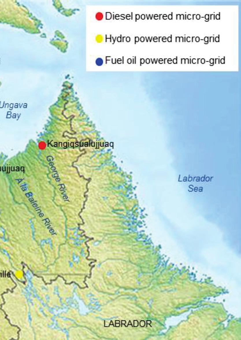
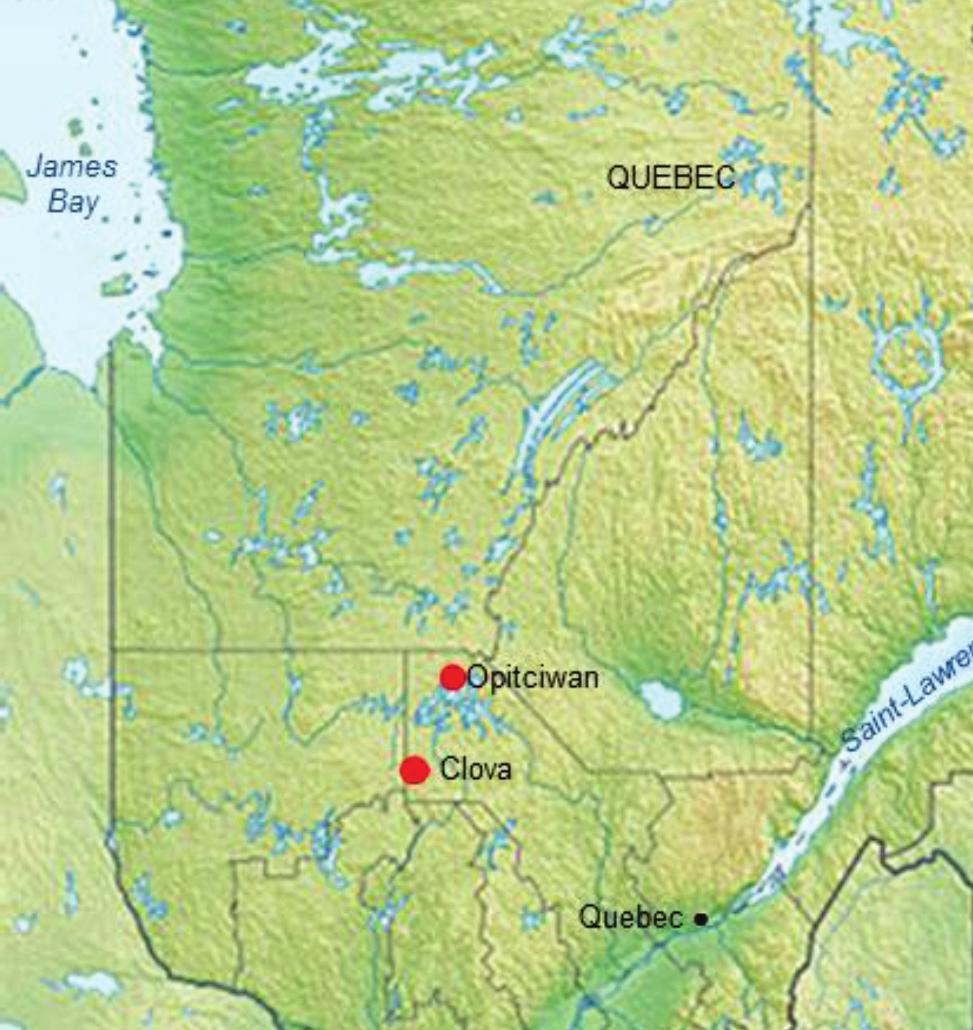
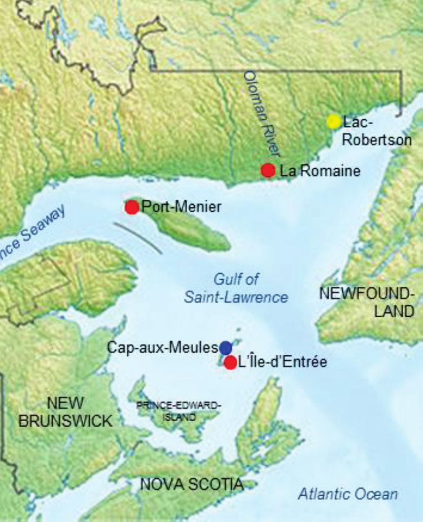
145 Figure 46. Remote micro-grids throughout Quebec 123