USE OF HYDRAULIC SIMULATION SOFTWARE TO EVALUATE FUTURE INFRASTRUCTURE UPGRADES FOR A MUNICIPAL WATER DISTRIBUTION SYSTEM IN BEGGS, OKLAHOMA

Transcription

1 USE OF HYDRAULIC SIMULATION SOFTWARE TO EVALUATE FUTURE INFRASTRUCTURE UPGRADES FOR A MUNICIPAL WATER DISTRIBUTION SYSTEM IN BEGGS, OKLAHOMA By MICHAEL C. LEA Bachelor of Science in Chemical Engineering Ohio State University Columbus, Ohio 2000 Submitted to the Faculty of the Graduate College of the Oklahoma State University in partial fulfillment of the requirements for the Degree of MASTER OF SCIENCE May, 2009

2 USE OF HYDRAULIC SIMULATION SOFTWARE TO EVALUATE FUTURE INFRASTRUCTURE UPGRADES FOR A MUNICIPAL WATER DISTRIBUTION SYSTEM IN BEGGS, OK Thesis Approved: Dr. Dee Ann Sanders Thesis Adviser Dr. John Veenstra Dr. Arthur Stoecker Dr. A. Gordon Emslie Dean of the Graduate College ii

3 ACKNOWLEDGMENTS I would like to thank Dr. Dee Ann Sanders for readily providing to me her knowledge and guidance throughout all stages of this project. I m happy to have worked with you as my thesis advisor. I would also like to thank Dr. Art Stoecker for sharing his time and efforts, especially his extensive help in managing project data. This thesis is based on elements of a larger project, funded through the Oklahoma Water Resources Research Institute, which aims to create a decision support model for water distribution infrastructure upgrades in rural Oklahoma. I want to thank project Team Lead, Dr. Brian Whitacre, and the five research assistants other than myself for all their contributions to our project. Fellow Research Assistants: Ernest Atta-Asiamah, Neha Bhadbhade, Deepayan Debnath, Jong San Choi, and Sara Senyondo. I would like to acknowledge Cliff Speer, Beggs Municipal Water Director, who provided to me the majority of my information about Beggs water distribution as it exists today. Also, Beggs Water Treatment Plant Manager David Brown provided similar assistance with respect to water treatment, and Amos Gaines, who maintains the pipeline distribution system, agreed to examine my final Beggs Year 2008 pipeline layout. I thank all of you. iii

4 I would like to thank my parents, John and Mary Lea, for all their support throughout my secondary education pursuits, and specifically to thank my father for his time and assistance provided during our conversations concerning this thesis. Lastly, I must acknowledge the faculty and staff of the Civil & Environmental Engineering College as a whole for their roles in providing to me opportunity and the necessary tools in preparation for my entry into the Environmental Engineering field. iv

5 TABLE OF CONTENTS Chapter Page I. INTRODUCTION...1 Purpose...1 Project Background - General...2 Project Background Site Description...4 II. REVIEW OF LITERATURE...7 Water System Design Principles...7 Components of the Hydraulic Model...10 Hydraulic Simulation Software...13 III. METHODOLOGY...16 Data Collection...16 Creating a Basic Software Model of the Pipeline Layout...19 Assign Populations to Nodes by Using Google Earth...24 Convert Population Data for Each Node Into a Water Demand...24 Hydraulic Modeling Using EPANET2 (Version )...27 IV. ANALYZING FINDINGS AND DEVELOPING SOLUTIONS...36 Analysis of Year 2008 Beggs...36 Peak Analysis...43 Diurnal Analysis...51 Analysis of Year 2050 Beggs...54 Peak Analysis...57 Diurnal Analysis...60 v

6 Chapter Page V. CONCLUSIONS AND RECOMMENDATIONS...63 Year Year Recommendations for Further Study...67 REFERENCES...69 APPENDICES...71 Appendix A: Example of Calculations for Adding Water Demands to Nodes...72 Appendix B: Calculations for Determining Pipe Lengths...73 Appendix C: Calculation of Elevated Main Tower Height...74 Appendix D: Peerless Pump Curve...75 Appendix E: Summary Table of Simulation Results...76 Appendix F: Determination of Beggs Average Daily Water Demand...77 Appendix G: Graphs of High Water Age Nodes Reaching Steady-state...78 Appendix H: Time Patterns...79 Appendix I: Year 2008 Suggested System Additions /Modifications...81 Appendix J: Process Control Rules...83 Appendix K: Year 2050 Suggested System Additions /Modifications...85 Appendix L: Final Diurnal EPANET *.inp Files...87 vi

7 LIST OF TABLES Table Page Table 1 Roughness Coefficients for New Pipe...32 Table 2 Test Showing C = 81.4 Simulates Constricting Pipe Diameter by 16.34% 33 Table 3 Test Showing C = Simulates Constricting Pipe Diameter by 12%...34 vii

8 LIST OF FIGURES Figure Page Figure 1 Beggs WTP...5 Figure 2 Beggs Pump Station...5 Figure 3 Beggs Elevated Water Tower...5 Figure 4 Beggs Underground Water Tank...5 Figure 5 Map of Beggs...6 Figure 6 Physical Components in a Water Distribution System...10 Figure 7 Typical Pump Head and Efficiency Curves...12 Figure 8 EPANET Graphical User Interface for a Tutorial Model...15 Figure 9 Screenshot of EPANET-Z after Adding the Basic Pipeline...21 Figure 10 Use of Google Earth to View Census Block Boundaries...23 Figure 11 8-Point Pump Curve for Pump Station Pump...30 Figure 12 Beggs Pumps...38 Figure 13 Flow Rate Patterns When Pump Is Active...39 Figure 14 Pipeline Additions to Accommodate Fireflows for the 2008 System...47 Figure 15 Schematic of Added Hilltop Tower and Related Pipes...50 Figure 16 Diurnal Time Pattern Used...52 Figure 17 Pump Curve for Year 2050 Peak Analysis...58 Figure 18 Recommended Year 2050 Beggs Pipeline Layout...60 viii

9 CHAPTER I INTRODUCTION Purpose This study directly addresses the steps required to assess Beggs water distribution system s current and future drinking water usage needs, required distribution infrastructure, and alternative solutions for providing increased or otherwise improved water distribution. This requires the effective use of hydraulic simulation software and population projections. Detailed equipment design is not within the scope of this study or the larger Oklahoma State project on which this study is based. Although a detailed cost analysis will be completed for the broader Oklahoma State project, this study will rely on more qualitative comparisons of implementation costs for each alternative. At the conclusion of this report, recommendations will be presented and justified based on the likely goals of decision makers and the appropriate legal regulations. This study utilized hydraulic simulation software to calculate system water quality, flows, and pressures for current conditions as well as possible future alternatives. An ancillary goal of this study was to ensure that the methodology is economical and accessible for others who would like to use this report as a guide to develop their own rural water distribution system analysis. Accordingly, this study uses free software developed by the EPA, called EPANET2, for hydraulic simulation, as opposed to any of 1

10 the other software solutions that must be purchased and can have a higher learning curve. EPANET2 is discussed in greater detail later in this report. There are potentially useful considerations that this report does not discuss because they stray from the focus of this study, which is to improve delivery of potable water through use of hydraulic software simulation. For example, issues such as access for maintenance, minimum spacing of shutoff valves, availability and capacity of auxiliary power, the probable duration of power failure, and the promptness with which repairs can be made, among other multidisciplinary concerns, lie outside the scope of this study. Another goal of this study was to effectively document the data gathering process because this first step can be especially difficult when working with rural water districts that do not have detailed records. Project Background General The Environmental Protection Agency s 1999 Drinking Water Infrastructure Needs survey estimated that Oklahoma will need 2.7 billion dollars to update their infrastructure in the next 20 years, of which 720 million dollars will be required for systems serving fewer than ten thousand people (Sanders, et al. 2008). Many rural water systems have unique needs and struggle with various aspects of planning for the future of their infrastructure, including assessments of its current status and what improvements or consolidation efforts are needed to accommodate future population/industry growth (Sanders, et al. 2008). Funding limitations of such rural communities require an economical approach to analyzing and creating a plan for 2

11 infrastructure upgrades. Unfortunately, rural communities often have incomplete records. This introduces difficulty in assessing the water district s current status. This study consists of elements from a broader project that is being carried out by a group of professors and research assistants, including myself, at Oklahoma State University. This broader project aims to create an accessible, cost-effective methodology to provide assistance to rural water systems for planning and updating their water supply infrastructure. The Oklahoma Water Resources Research Institute (OWRRI) funded and set the scope for the general Oklahoma State project, which includes the water distribution study carried out for this report. The city of Beggs was chosen for this study because it fit the characteristics of a typical rural water district in need of assistance with water system improvements. For the purposes of this study, rural refers to a town or community with fewer than 10,000 persons that is not a suburb of a larger city people currently reside in Beggs, OK, accounting for 650 water service connections (ODEQ 2008). The majority of Beggs water distribution system was installed during or before the early 1960 s and has accumulated a high degree of bacterial, rust-related, and/or mineral deposits within its pipelines (Speer 2008). Beggs water treatment plant (WTP) currently cannot be operated at its rated maximum treatment flow rate without violating water quality standards for total organic carbon (TOC). This difficulty limits the maximum flow rate of water available for distribution over extended time periods, though this has not been a problem to date. Violations of halogenated alkanes regulations within the distribution system have typically occurred several times per year, possibly due to excessive total organic carbon (ODEQ 2008). 3

12 Project Background Site Description The city of Beggs occupies approximately 4.3 square miles within Okmulgee County, Oklahoma, and lies approximately 25 miles south of Tulsa, OK (USGS 2008). The latest U.S. Census determined that 1364 persons resided in Beggs in the year The Oklahoma Department of Commerce predicts a population of 1650 persons by the year 2030 (OSDC 2008). Beggs Lake, which serves as the city s public drinking water supply source, has provided an ample supply of water throughout droughts, including the drought that occurred recently during late 2005 to early 2006, when the WTP intake at the lake did not have to be lowered to accommodate reduced lake levels (Speer 2008). Beggs WTP (Figure 1), built in 1995, lies adjacent to Beggs Lake and provides treated water to an underground tank (Figure 2) that is adjacent to the Pump Station located at the outskirts of the main city. This Pump Station (Figure 3) delivers water from a 150,000 gal intermediate underground tank to the city s only elevated water tower. This elevated, 50,000 gal main tower (Figure 4), located in central Beggs, serves water to the city by gravity feed. A chlorine booster pump is located at the Pump Station to ensure adequate chlorine residuals because the underground tank is large enough to create water age problems otherwise. The majority of Beggs' water pipelines were installed during or before the early 1960 s and are composed of cast iron. Exact installation dates are currently unavailable or are unknown to the city of Beggs. Newer pipeline additions, composed of polyvinyl chloride (PVC), have been installed within the last 10 years to serve the new Beggs school in the northeast and the developing Hilltop neighborhood located to the southeast of Beggs, among other locations. All of Beggs pipelines are either 2, 3, 4 (the majority), or 6 in diameter, with the lone exception being the 8 4

13 pipeline that connects the WTP to the pump station s underground tank (Speer 2008). The Beggs distribution system is modeled as if there were no emitters, which are orifices that discharge to the atmosphere at whatever flow rate is delivered to it. The school uses 50,000 gal/month during the school year (Speer 2008). No major sources of industrial water used were identified. Figure 5 shows a map of the city with landmarks labeled. The locations of highest elevation within Beggs are located near the elevated water tower and also in southeastern Beggs in the Hilltop region. Figure 1 Beggs WTP Figure 2 Beggs Underground Water Tank Figure 3 Beggs Pump Station Figure 4 Beggs Elevated Water Tower 5

14 Figure 5 Map of Beggs 6

15 CHAPTER II REVIEW OF LITERATURE Water System Design Principles Nearly 80 to 85% of a water supply project s cost is due to the distribution system; therefore, using a rational system for distribution design will provide significant savings (Swamee 2008). Factors that should be considered for optimal distribution system design include the following: a determination of the required lifespan of the designed additions projections on population commercial, and industrial growth that will allow for projections on future water needs the current per capita water consumption peak factors for water demand the minimum/maximum allowable water pressures and pipe sizes reliability considerations (Swamee 2008) Additionally, a water distribution system should have adequate water storage available to ensure that extended periods of high usage do not require more water flow than the system can provide. Water storage requirements should take into consideration the peak 7

16 daily water use, the maximum day demand plus the required fire flow, the capacity of the normal and standby pumping equipment, the availability and capacity of auxiliary power, the probable duration of power failure, and the promptness with which repairs can be made (Salvato 1992). Also, it is recommended that half of a maximum day s demand be contained as water storage, and that at least half of that water storage be contained in elevated towers to ensure that water pressures can be maintained during short-term, high demand events such as a structure fire that must be extinguished. Water mains should be designed on the basis of 4 to 6 fps liquid velocity with maximums of 10 to 20 fps (Salvato 1992). Design velocities as high as 10 to 15 fps are not unusual. Author Joseph Salvato suggests that a minimum water pressure of 35 psi is preferred, though a minimum of 20 psi may be acceptable (Salvato 1992). Oklahoma Public Water Safety Construction Standards require that all mains have no less than a 6 diameter (ODEQ 2008). The Insurance Services Office (ISO) develops standards by which fire fighting capabilities can be classified for the purpose of setting insurance premiums in the United States. ISO utilizes a tiered Fire Suppression Rating Schedule to classify firefighting capabilities. Beggs decision makers currently have chosen a goal of a Class 8 Public Protection Classification. Class 10 is the minimum for ISO recognition and Class 1 is the highest. To achieve Class 8 status, ISO requires that all locations being considered for structure insurance have the capability to be served by 250 gpm fireflows at peak daily water demand conditions while maintaining a minimum of 20 psi (ISO Mitigation Online 2008). Improvements in the capability of a water distribution system to deliver water during a fire event will typically result in lower insurance premiums (Salvato 1992). 8

17 Even if the resulting savings on insurance premiums does not financially justify the cost to improve the fire protection class, the greater safety to life and property makes the value of improved fire protection more persuasive (Salvato 1992). Installed municipal water pipes must have a protective inner surface covering to prevent corrosion (Salvato 1992). Design velocities within the pipes at a pump station should be ft/s. It is a common practice of many water companies in the United States to design pipe diameters based on average hour demands rather than maximum hour demands of the maximum consumption month. This helps keep the investment costs associated with installing new pipelines reasonable and seems to provide a good tradeoff between these costs and reliability concerns (Trifunovic 2006). A pump station s water pumps must have the ability to fill the system s elevated water towers within a 6-12 hour time period (Salvato 1992). Some head loss is expected at the pump station. Friction, pipe bends, and valves are the largest sources of head losses attributed to the pump station (ODEQ 2008). Water hammer can result from a very rapid acceleration of cessation of flow, resulting in very large momentary positive and negative pressure changes (surges) from normal (Salvato 1992). Dead-ends should be eliminated to avoid problems with high water age and insufficient water pressures (ODEQ 2008). House count, census records, and predictions of future populations can be used to develop a forecast of future water demand (Swamee 2008). Though heuristics are available, the selection of a suitable peak factor ultimately requires the judgment of the engineer (Swamee 2008). To design the system for worst-case scenario, the peak factor can be based on the ratio of hourly demand of the maximum day of the maximum month 9

18 to average hourly demand (Swamee 2008). For a city with a population of less than 2000 persons, a peak factor of 5 should be suitable (Swamee et al. 2008). Components of the Hydraulic Model Hydraulic modeling of a water distribution system has proven to be an effective and reliable technology to analyze an existing or proposed system under a wide range of hydraulic conditions. Such hydraulic modeling is most easily accomplished by computer software that utilizes laws of conservation of mass and energy to determine pressure and flow distributions throughout the network (Mays 2000). Conservation of mass dictates that for each node the algebraic sum of flows must equal zero. Conservation of energy requires that along each closed loop, the accumulated energy loss must be zero (Mays 2000). A hydraulic model of a water distribution system is represented as a collection of links connected to nodes. The links represent pipes, pumps, and control valves and the nodes represent junctions, tanks, and reservoirs. Figure 6 below illustrates an example system of nodes and the links that connect them (Rossman 2000). Figure 6 - Physical Components in a Water Distribution System (Rossman 2000) 10

19 Each node contains information about its elevation, water demand, and initial water quality. A successfully run simulation computes hydraulic head, water pressure, and water quality for each node at various times. The solution for heads and flows at a particular point in time involves simultaneously solving the conservation of flow equation for each junction and the head loss relationship across each link in the network. This process, known as hydraulically balancing the network, requires using an iterative technique to solve the nonlinear equations involved (Rossman 2000). Reservoirs are nodes that represent an infinite external source or sink of water to the network. They are used to model such things as lakes, rivers, groundwater aquifers, and tie-ins to other systems. Tanks are nodes with storage capacity, where the volume of stored water can vary with time during a simulation. Pipes are links that convey water from one point in the network to another. The software used for this study, EPANET2, assumes that all pipes are full at all times. The principal hydraulic input parameters for pipes are start/end nodes, diameter, length, and roughness coefficient for head loss. Principal water quality parameters related to pipes are the bulk reaction coefficient and wall reaction coefficient. The section of this report titled Hydraulic Modeling Using EPANET2 discusses coefficients in more detail. Valves are links that limit the pressure or flow at a specific point in the network. The principal input parameters for valves are start/end nodes, diameter, initial open/closed status, and a flow/pressure control point setting to allow for automated control of the valve s open/closed status. Upon completion of a successful simulation, modeling software can calculate flow rate and head loss for each valve. The EPANET software allows for process controls of various equipment that can affect flows, using either pre-defined controls or using rule-based 11

20 controls that require programming language statements to be written. Pumps are links that impart energy to a fluid, thereby raising its hydraulic head. The principal input parameters for a pump are its start and end nodes and its pump curve (Rossman 2000), which represents the combination of heads and flows that the pump can produce (Figure 7). Output parameters for pumps are flow and head gain (Rossman 2000). A pump efficiency curve (Figure 6) is used for energy use calculations and describes the relationship between power efficiency and pump flow. The location representing the most energy efficient operating point occurs at the apex, or maximum, of the efficiency curve (Swamee 2008). Figure 7 Typical Pump Head and Efficiency Curves (Hegberg 1999) Hydraulic modeling software tracks the fate of discrete parcels of water as they move along pipes and mix together at junctions between fixed-length time steps. It calculates the concentration and size for each of a series of non-overlapping segments of water filling each pipe of the network. Water quality can be analyzed as a fate and 12

21 concentration of a reactive chemical, or in terms of water age, which refers to the average length of time that water at a specific location has been circulating within the pipeline (Rossman 2000). For each water quality time step, the contents of each water segment are subjected to reaction, and a cumulative account is kept of the total mass and flow volume entering each node. The new positions of the segments are then updated (Rossman 2000). Water at nodes can have a slightly higher age than water along the pipes they are a part of if they are dead ends because they represent the age at the end of the pipe rather than the average age along a pipe s length. Correspondingly, water within pipes can have higher age than water at nodes if water flow is continually reversing direction within the pipe, causing water near the middle of the pipe to be the oldest. Dead zones and short circuiting within tanks can be modeled by creating an imaginary second compartment within a tank. The tank is assumed to have both its inlet and its outlet located at the first compartment, and each compartment is assumed to be individually completely mixed. Routing input water directly from the input to the output without sending overflow water from the first compartment to the second compartment models short circuiting. Additionally, assigning dead zone properties to the second compartment simulates a dead zone within this second compartment (Rossman 2000). Hydraulic Simulation Software Researchers and engineers use hydraulic simulation software to better understand properties of a water system and to investigate alternatives without the need for rigorous hand calculations for each alternative. In the 1990 s, the EPA s Water Supply and Water Resources Division developed a software program to perform extended-period simulation 13

22 of the hydraulic and water quality behavior within pressurized pipe networks (EPA 2008). This software, EPANET2, is free of charge and available for download at the EPA website, There is a modification of EPANET2 called EPANET-Z, which will be discussed later. Within this study, these hydraulic modeling programs will be generically referred to as EPANET unless a distinction between the two is necessary (EPA 2008). EPANET provides a fully equipped, extended-period hydraulic analysis package can do the following: Compute friction head loss using the Hazen-Williams, the Darcy Weisbach, or the Chezy-Manning head loss formula Include minor head losses for bends, fittings, etc. Model constant or variable speed pumps Compute pumping energy and cost Model various types of valves, including shutoff, check, pressure regulating, and flow control Consider multiple demand categories at nodes, each with its own pattern of time variation Model pressure-dependent flow issuing from emitters (sprinkler heads) Base system operation on simple tank level or timer controls as well as on complex rule-based controls Model the age of water throughout a network (EPA 2008) EPANET software can assist with pipe, pump, and valve placement and sizing, energy minimization, fire flow analysis, vulnerability studies, and operator training (EPA 2008). Figure 8 shows a screenshot of the EPANET graphical user interface. 14

23 Figure 8 EPANET Graphical User Interface for a Tutorial Model 15

24 CHAPTER III METHODOLOGY Data Collection The scope of this study encompasses rural Public Drinking Water Supply districts with either deteriorated infrastructure and/or a future population growth that will require infrastructure upgrades. After identifying a community that fits these qualifications, the first step taken was to independently research the target water district. Though rural communities often lack detailed records of their infrastructure and water usage, there are resources available that provide reliable information on even the smallest of water districts. A government website, provides current population estimates and population projections (USCS 2008). The U.S. Census Bureau website, American Factfinder, provides population data such as the number of persons per household, which is equal to 2.51 in Beggs, OK (USCB 2008). The Oklahoma Department of Commerce, is an additional source for population data (ODOC 2008). Population data at the census block level can be obtained from the website of Environmental Research Systems Institute, Inc. (ESRI), which is a privately owned company and one of the more prominent developers of Geographic Information Systems (GIS) software. 16

25 Block level data is the smallest division of area for which the U.S. Census data is available to the public (ESRI 2008). To download the census block boundaries as *.shp files, the user must navigate to and download Census Blocks 2000, which is a 462 kb file for Okmulgee County. To download census block population metadata, navigate to and download Census Block Demographics (SF1), which is a 5.4mb file for Okmulgee County. An Oklahoma Department of Environmental Quality website, provides water quality sampling data, a record of quality violations, and other site-description information for water districts in Oklahoma (ODEQ 2008). The Oklahoma Water Resources Board (OWRB) website provides files of pipeline distribution layouts and associated metadata such as pipe diameters and system water demand for rural water districts. Unfortunately, some small cities (such as Beggs) that are not nominally considered to be rural water districts are not as well documented (OWRB 1998). A United States Geological Survey (USGS) website, called The National Map Seamless Server, provides elevation information, including a downloadable.adf file that contains all elevation data for any user-defined rectangular geographic area (USGS 2008). To download this file, the user must navigate to the website, choose View & Download United States Data, and then use the controls in the sidebar to zoom in to the geographic area of interest. The user then selects Define Rectangular Download Area and click-and-drags the mouse pointer over the area of interest. A pop-up window will appear that will allow the.adf file to be saved as a zipped file. The user can optionally first select Modify Data Request and change the National Elevation Dataset from 1 arc 17

26 second to 1/3 arc second to obtain a higher resolution for elevation data; however, I found that the default 1 arc second dataset yielded elevations that matched the 1/3 arc second dataset to within one decimal place in units of feet, so using the higher resolution dataset appeared to be unnecessary for purposes of this study. The higher resolution elevation data may not be available for all geographic areas. Following preliminary research, interviews were conducted with public officials, system managers, and the community to better understand the water system (Sanders, et al. 2008). Information collected included the following important issues: Problems the water district is currently having with their water supply such as inadequate flows, water quality, deposits on the inside of pipelines, etc. Water usage records (from treatment plant, water utility billing, or other sources). Any information about the potential for future population, commercial, or industrial growth. Equipment in service: towers, boosters, pumps, valves, tanks, etc. Water Treatment Plant and equipment specifications. Pipeline specifications such as pipeline layout drawings, diameters, lengths, etc. Contact information of those who work for the water district/city/county or otherwise that may provide useful information. Water pressure measurements at key locations Previous studies that relate to water or population distribution of the target community 18

27 Creating a Basic Software Model of the Pipeline Layout This section describes how the graphical user interface of EPANET and other software were used to create a basic pipeline layout, add necessary equipment, and incorporate data parameters such as elevations and water demands into a system model of a distribution system. Later, in the section titled Hydraulic Modeling Using EPANET2, choices of parameters required to hydraulically model the system will be discussed in more detail, including a discussion of the selection of hydraulic coefficients and various parameters for tanks and pumps. As discussed in the previous Data Collection section, because the OWRB website does not provide metadata.shp files for Beggs, OK, all parameters, such as pipe lengths, diameters, and locations, were researched or calculated and incorporated into the model manually. Software programs such as Microsoft Excel macros were utilized to automate portions of this process. The present-day conditions of the Beggs water distribution system were the first to be modeled. Later, future conditions were modeled. Digital pipeline layout maps were not available for Beggs, so instead, a hard copy of two pipeline layout maps was obtained from the municipal water director of Beggs. One map was drafted in the early 1960 s by an engineer, presumably following implementation of improvements to the system. The other map was created by a member of the Oklahoma Department of Environmental Quality (DEQ) after a drive around the streets of Beggs in which pipeline locations were identified by a city employee who maintains the pipeline system. Neither map was complete by itself, but between the two maps and input from the municipal water director, I pieced together the layout of the pipeline system as closely as possible. 19

28 Creating a basic digital layout of a pipeline requires only a list of all pipes in the system and the associated x,y-position coordinates for each pipe endpoint. Though this can be accomplished by manually entering columns of data into a simple text file, the EPANET-Z graphical user interface provides a more visually straightforward way to achieve this. EPANET-Z is a modification of EPANET2 that automatically incorporates internet-based maps, such as Google maps or Yahoo maps, as a background for the pipeline layout. Because EPANET-Z is an unofficial modification of EPA software, it should only be used to create or edit the pipeline system file, while EPANET2 should be used for final analysis. Using EPANET-Z s toolbar icons for node and link placement, each pipeline and pipe endpoint carefully placed by clicking directly onto the appropriate locations on the map background (Figure 9). Where necessary, vertices were placed to allow for pipe bends within one length of pipe. Unlike a node, the only data that can be assigned to a vertex is x,y-position and elevation data. The locations of water demand, which play a role in node placement, were added to the model to simulate the water consumed daily by the residents of Beggs. Although the most intricate way of modeling water demand is to place a node (which is the only type of object that can be assigned a water demand) at every location within the system where water is consumed, the system can be simplified by instead placing nodes at pipe junctions/endpoints and bends, with water demands within the proximity of each node being grouped and assigned to the appropriate node. Typically, this suggests that nodes need only be placed at each end of a straight portion of pipe; however, the software only calculates results for pressure and quality at node locations, so nodes were added along the length of any straight pipes at intermediate 20

29 locations where specific, calculated results were desired, such as locations where population density was large compared to surrounding areas. Figure 9 Screenshot of EPANET-Z after Adding the Basic Pipeline Beggs supplies water from an elevated main tower in central Beggs via gravity as well as from an underground tank at the outskirts of Beggs from which water is pumped. The Main Tower, underground tank, and Pump Station pump were added to the pipeline system. When placing the pump, it was necessary to orient it such that water flows in the correct direction. Setting water levels, pump curves, etc. for equipment will be discussed later within the section titled Hydraulic Modeling Using EPANET2. All pipeline and equipment parameters, such as water demand, pipe diameter, etc., were assigned to each pipe, node, and piece of equipment via a dialog box. Using these 21

30 dialog boxes, I manually added the individual pipe diameters for each pipe. The hydraulic software allowed for the editing of multiple pipes or nodes at once. The method for determining numerical values to enter for water demands is a multi-step process. Though location of water demand is primarily a function of the location of residents, it may also be necessary to consider industries, commercial businesses, or institutions that consume large quantities of water if decision making could be affected by their exclusion. The mayor and the municipal water director of Beggs identified no significant water consuming industry, businesses, or institutions, so the location of residents became the focus. Although a model can be created that assumes population is distributed evenly among any placed nodes such that each single node is assigned the same water demand, a more accurate representation can be obtained from block level census data. Google Earth provides an easy and effective way for visually representing block level census data; however, the.shp file for block level population boundaries (that can be obtained from the ESRI website (ESRI 2008) must first be converted to a Google Earth file with a.kml file extension using software called Shp2kml, which was developed by the same people who created the EPANET-Z modification (Zonum Solutions 2008). Because Shp2mkl and the ESRI website data are provided as is without liability by private entities, the U.S. Census Bureau website American Factfinder can be used to confirm the accuracy of the population data (USCB 2008). The opening screen of Shp2kml prompts the user for the source *.shp file, for which the WGS 1984 Global Definition is a suitable coordinate system. I proceeded through the various pages of options in Shp2kml, making sure to check-mark all fields 22

31 underneath Balloon Definition for the sake of clarity, otherwise, the default settings sufficed. Using Google Earth to open the.kml file generated by Shp2kml, I viewed the color-coded blocks of Beggs. Figure 10 shows a slightly zoomed-in view of these census blocks. Figure 10 Use of Google Earth to View Census Block Boundaries As mentioned previously in the Data Collection section, the other block level population file of importance is the Census Block Demographics (SF1) file, which has a file extension of.dbf and can be opened directly in Microsoft Excel as tables of population data organized by block. Block level populations were used to assign water demands to a particular node by the following method: 23

32 Assign Populations to Nodes using Google Earth and a Census Block.kml File Identify the population for a particular census block. Use the overhead map satellite view to visually identify and count each residence within the block. For each house, determine which node in the vicinity best represents the location of pipe from which its water is drawn. For each appropriate node, enter into the EPANET-Z dialog box Tag blank a value equal to the number of associated homes multiplied by the weighted fraction of population these homes account for within the census block. For example, for a census block with 4 homes and a population of 10 persons, entering 7.5 into the Tag blank for Node 12 serves as a notation that three out the block s four homes have been assigned to Node 12, because 10 persons multiplied by three-fourths equals 7.5 persons. NOTE: EPANET-Z does not utilize information entered into the Tag blank. The population value that has been entered into this Tag blank will be converted to water demand in gpm using Excel in a later step. Repeat the previous steps for all census blocks until all census block populations within the water district have been assigned to a node. Use EPANET-Z s export function to save the pipeline layout as an editable text file with an *.inp file extension. Convert Population Data for Each Node into a Water Demand Open the saved *.inp file in a text editor such as Wordpad, then copy the [TAGS] section and paste the data into an empty Excel spreadsheet. Within Excel, sum all population values in the [Tag] section to find what total population was assigned to the nodes. This value should equal the city s total population. In another new column and for each node, multiply each node s assigned population by the same conversion factor such that this entire new column sums to a value of 100. These new values represent the water demand in gpm assigned to each node; therefore the total water demand of the city is set to 100 gpm with each node being accountable for a different fraction of that total demand. NOTE: Now, within the EPANET software, if you want to simulate a system with a total water demand of gpm, you should enter into the Analysis Options/Demand Multiplier blank. 24

33 Replace the original demand data in the [JUNCTIONS] section of the *.inp file with the new demand data (that was calculated in the previous step). To achieve this using Excel, copy the entire [JUNCTIONS] section into an empty Excel spreadsheet, then paste the new demand values over the original demand values, then save the [JUNCTIONS] spreadsheet as a Formatted Text (Space Delimited) *.prn file. Open this *.prn file containing the new data in a new instance of Wordpad. Copy the contents of the *.prn file, and then switch to the original instance of Wordpad and paste over the original [JUNCTIONS] section. Save the adjusted *.inp in Wordpad to complete the process. This newly saved *.inp file now has proper values for water demand entered at each node. Appendix A shows the Excel spreadsheet used to calculate and add water demands to each node by following steps similar to those above. Other parameters such as pipe lengths and elevations were determined and incorporated into the model. Elevation differences are directly measured as static hydraulic head loss. Elevations must also be taken into account when determining pipe lengths because distribution systems are typically not built on completely flat terrain. Although the National Map Seamless Server website (USGS 2008) can be used to find the elevation at any single x,y-coordinate location for manual entry, it also provides a downloadable.adf file that contains all elevations contained within a user-defined rectangular geographic area, which can then be opened using GIS software, such as GlobalMapper, to automate the addition of elevation data to each node in the system. I found that an even quicker way to add elevation data to the original EPANET *.inp file was to use the internet-based software application EPAElevations (Zonum Solutions 2008). This applet used the EPANET *.inp file as its input and it outputted a modified *.inp with elevations appended. The National Map Seamless Server website (USGS 2008) was then used to confirm the accuracy of the EPAElevations applet. The creator 25

34 of the EPAElevations applet used the same USGS source for elevation data that The National Map Seamless Server uses (Zonum Solutions 2008). An increase in pipe length results in an increase in frictional hydraulic head loss, which in turn causes pressure drop across a pipe. EPANET contains a function that is supposed to automatically calculate pipe lengths based on pipe endpoints; however, the software inexplicably calculated pipe lengths that were incorrect by as much as - 20% for pipelines of a mostly longitudinal orientation and +20% for latitudinal pipelines, so pipe lengths had to be calculated manually. 1 decimal degree at the equator correlates to approximately 22 miles ( mile circumference (Rosenberg, et al. 2002) divided by 360 ), while 1 decimal degree near the Geographic North Pole correlates to a negligible length, indicating that the conversion of decimal degrees to latitudinal length is dependent on where the site of interest lies along the Earth s longitude. However, because Beggs is only approximately 2 miles across from south to north, which is a length that is negligible relative to the circumferential distance from equator to pole, and because Oklahoma does not lie close to the Geographical North Pole, the effect the Earth s curvature has on the conversion of degree coordinates to lengths was neglected. Using Google Earth s ruler utility to test this assertion revealed < 0.1% discrepancy between the degrees/feet ratio at Beggs southernmost and northernmost points. Note that the Earth s curvature has absolutely no effect on such conversion calculations for longitudinal spans of length because of the way longitudinal lines are defined. Accordingly, the USGS National Map Seamless Server s (USGS 2008) length calculator was used to find that 0.01 E/W decimal degrees is equivalent to ft, and 0.01 N/W decimal degrees is equivalent to ft at Beggs, OK. On this basis, an Excel 26

35 spreadsheet was used to convert the difference between each pipe s x,y,z-location endpoints as decimal degrees and elevations into pipe length in units of feet. I converted x-coordinate degree differences into lengths, and then y-coordinate degree differences into lengths, and from those lengths resolved the x,y-plane hypotenuse using Pythagoras Theorem. However, some pipes have endpoints that occur at very different elevations, such as the pipe that is routed up the elevated water tower. In such cases, accounting for elevation differences was necessary to calculate pipe length accurately. Once again, Pythagoras Theorem was used to resolve true pipe lengths as a function of the x,y-plane projection length and the pipe s elevation change. Using the same method that was previously used for adding water demands to nodes (by saving the important Excel data as a Formatted Text Space Delimited *.prn file), pipe lengths were copy/pasted into the EPANET *.inp file. Though the applet that the USGS National Map Seamless Server (USGS 2008) uses does not always present its maps visually to scale, the numerical data obtained should still be accurate. Appendix B contains the Excel printout showing an example of the process for calculating correct pipe lengths. Hydraulic Modeling Using EPANET2 (Version ) The previous section described the input of nodes, equipment, pipeline links, pipeline diameters, water demand, and node elevations to create a basic model. This section describes the process of using EPANET functions/commands to run the model, as well as discusses the choice of parameters, e.g. equation constants, that best model the hydraulic system. 27

36 Each type of equipment (tanks, pumps, valves, etc.) added to the system model has particular parameters that must be set. Each tank has a shape, volume, initial water level, elevation to tank bottom, and mixing model that must be either determined or assumed. Beggs has two water tanks. The first is a large, cylindrical underground tank that lies at a low point within Beggs, provides flow equalization from the WTP, and is the largest water storage volume within Beggs at 150,000 gal. It has a side wall depth of 20 ft, but only 17 ft is beneath ground surface. I chose to model the underground tank as an infinite reservoir for three reasons: The scope of my thesis includes water distribution rather than WTP treatment processes, so eliminating the WTP equipment from my model decreased sources of error for troubleshooting. This also resulted in making the underground tank the first element for water flow within my model. The first element within a hydraulic software model must always be an infinite reservoir (Rossman 2000). Over the city s history and during droughts, the city of Beggs has had ample treated water supply from the underground tank and ample source water for WTP treatment from Beggs Lake. This supports the assumption that the underground tank can be considered an infinite source (Speer 2008). The only descriptive parameter for a reservoir within EPANET is the height to the upper water level expressed as elevation. To be conservative, it was assumed that the underground tank (that models a reservoir) always maintained 1.5 ft of water level. This models the worst-case scenario for providing hydraulic head because the underground tank s outlet was assumed to be positioned 1.5 ft from its base to avoid withdrawing collected particulate materials from the bottom of the tank. This choice corresponded to a water level of 15.5 ft below ground surface. The second tank is the centrally located main water tower which serves water by gravity pressure throughout Beggs, is elevated 28

37 75 ft above ground level, and also is located at a geographic high point within Beggs. The elevated water tower s 75 ft of height to the tank s bottom and 20 ft diameter were entered into the tank s EPANET dialog box for parameter entry. Because Beggs city employees reported that the tank s volume is 50,000 gal, but were not aware of its height, a tank height of 21.3 ft was calculated that corresponds to a 50,000 gal volume (Appendix C). By visual inspection, this height seemed reasonable to me. Though EPANET is capable of modeling oddly shaped tanks, the elevated tank in Beggs has a simple cylindrical shape, which is the default shape assumed by EPANET. For the elevated tank, an initial water level equal to half its height was assumed, which allowed the model to be run without having any pump control conditions (which are discussed later) triggered at or near time t = 0. Lastly, I assumed that the water within the elevated tank was perfectly mixed because I found no significant reason throughout my research to assume otherwise, e.g. an improperly designed tank with both its inlet and outlet located at its base such that short-circuiting can occur. Pumps have only one descriptive parameter that can be assigned within EPANET, the pump curve. Ideally, the pump curve should be obtained from the pump s documentation or by contacting the manufacturer. Appendix D illustrates the pump curve for the Pump Station pump in Beggs. The Pump Station pumps (there are two for redundancy) were installed in the late 1970 s. For this study, the pump curve was manually entered as a series of data pairs that represent points on the curve. Figure 11 shows the multi-point pump curve used. 29

38 Figure 11 8-point Pump Curve for Pump Station Pump EPANET-Z Version 0.5 cannot be used to create a pump curve, so EPANET2 was used instead. Although EPANET-Z will open pipeline *.inp files that contain pumps, execute the model, and save any pipeline changes properly, it cannot be used to create or edit the shape of a pump curve. The Pump Station pump must be controlled to shut off if the elevated Main Tower nears full capacity (maximum water level = ft) and the pump must turn back on if the elevated main tower capacity gets too low. Currently, this pump at the Beggs Pump Station operates with process controls such that it turns off when the elevated Main Tower reaches 71.8% of its maximum capacity and turns back on when it drops below 47% of its maximum capacity (Speer 2008). This ensures that the Main Tower never becomes completely full and allows the pump to be off some of the time. This extends its useful life and helps to ensure that the Main Tower never empties, which leaves a volume 30

39 of water available for fireflows at all times. To implement this process control into the model, I opened the Rule Based Controls in the browser and entered the following code: RULE 1 IF TANK 6 LEVEL ABOVE THEN PUMP 4 STATUS IS CLOSED RULE 2 IF TANK 6 LEVEL BELOW 13 THEN PUMP 4 STATUS IS OPEN Hydraulic simulation software uses many equations with various constants to model its system. For this study, the only coefficient of concern was pipe roughness. Setting minor loss coefficients for each pipe to a slightly high, but typical, value such as 2.0 (Rossman 2000) provided only a 1% change to pressures throughout the Beggs system. Considering the lack of records/data for Beggs water system, such as not having a complete pipeline layout to work with, this effect of minor losses on hydraulic head losses was deemed comparatively insignificant. Accordingly, the Loss Coeff. blank in each pipe s dialog box was left empty. Pipe roughness coefficients can hypothetically be calculated by measuring the water pressure and flow at each end of a single, uninterrupted, straight pipe and using the Bernoulli equation to resolve the frictional head losses; however, an investigation into the practicality of this method revealed that over the length of a 1000 ft schedule 40 steel pipe, the pressure drop can be as low as 0.7 psi (Crane Engineering 1976), which is likely too small of a change to be measured by a typical pressure gauge that may only be capable of measuring water pressures to within +/- 0.5 psi. Even though the aged pipelines at Beggs have a more severe roughness than the schedule 40 steel pipe being referenced, the more appropriate choice for this project is 31

40 to apply typical values from literature. Beggs municipal water department did not complete water pressure testing in time for inclusion in this thesis, so I initially considered entering reference roughness values for newly installed pipes by using values from Table 1. This suggested setting the roughness coefficient to C = 100 as an initial estimation for older pipe; however, these values were not ultimately used, as explained below. Table 1 Roughness Coefficients for New Pipe (Rossman 2000) The majority of the pipe within Beggs is 45+ years old or more. At the time of this study, there were no recently dug up pipes available to inspect for deposits, though the Beggs Municipal Water director and other pipeline maintenance employees reported that among the pipes they had seen dug up in the past, as much as one-sixth of the pipe s diameter had been constricted by extreme buildup of deposits. This observation was used as the basis for setting roughness coefficients for this study even though the lack of direct measurement serves as a source of uncertainty. To test how older pipe could be simulated by adjusting the pipe roughness coefficient, I created a new pipeline system following EPANET s tutorial example (Fig. 7) and edited one straight, level pipe with a roughness coefficient C=130 (typical for new 32

41 cast iron pipe (Rossman 2000)) to have a diameter that was only one-sixth of its original diameter and noted that the unit head loss across its length was the same as if a roughness coefficient C=81.4 and 100% original diameter had been used instead. From this test, I concluded that for old pipes within Beggs, setting the pipe roughness coefficient equal to 81.4 will best simulate pipe deposits which cause hydraulic head reducing friction and constricted flow. This test was carried out at multiple pipe diameters, flow rates, and times to ensure that the assumption of C = 81.4 for old pipe was valid under an appropriate range of conditions. The simulated pipe used for the test was 3000 ft long with a constant elevation of 700 ft. The test results are listed below in Table 2. Table 2 - Test Showing C = 81.4 Simulates Constricting Pipe Diameter by 16.34% Test A %Δ Test B %Δ Test C %Δ Test D %Δ Diameter, in Roughness, C Head loss, ft/kft Flow rate, gpm Time, h Similarly, a roughness of simulated a further reduction in pipe diameter of approximately one-eighth over the next 42 years until Year 2050 (Table 3). This slightly lesser reduction of pipe diameter was chosen because water velocities are expected to be higher in the future, which helps to reduce deposition (Trifunovic 2006), and the age of the current oldest pipes in Beggs was assumed to be 45 years at minimum, as opposed to a future additional age of only 42 years at maximum. 33

42 Table 3 - Test Showing C = Simulates Constricting Pipe Diameter by 12% Test A %Δ Test B %Δ Diameter, in Roughness, C Head loss, ft/kft Flow rate, gpm Time, h There are many settings within EPANET that can be set to determine how the model is executed. Unless otherwise mentioned in this thesis, EPANET s default settings were used. Some settings, however, require the discretion of the user. Through trial and error and viewing time series plots of results, 96 hours was determined to be enough time for the system to reach steady-state. This duration was set in the Times/Options dialog box. Water age was the parameter that took the longest to reach equilibrium. This was set as the water quality parameter of interest by selecting Age in the Quality blank for Hydraulics /Options. After the satisfactory execution of the hydraulic model for the water system s current conditions, a model was developed for future conditions, which in the case of Beggs, refers to the projected increase of water demand due to increased population only; industrial growth is not currently expected (Speer 2008). An understanding of the geographic population distribution is not necessary to make a simple projection of total future population; however, it can help to inform where to best locate the water demand nodes for a simulation. With respect to population projection, The Oklahoma Dept. of Commerce lists Beggs population at 1364 persons in the year 2007, which is no change from the 2000 US Census population; however, another Oklahoma Dept. of Commerce document predicts that the Beggs population will be 1450 in the year 2010 and 1650 in the year 2030, increasing by 100 persons per decade from the years (OSDC 34

43 2008). Because the OSU team for the larger project determined that research into rural water system upgrades should plan for future needs until the Year 2050, this study also followed that time frame. Extrapolating the trend by 100 persons per decade yielded a projected Beggs population of 1850 persons in the year The 35.6% percent increase of population from 1364 to 1850 persons directly correlates to a 35.6% higher water demand. As a result, the Year 2050 total water demand was projected to be gpm, which was 35.6% higher than the Year 2008 demand of gpm. 35

44 CHAPTER IV ANALYZING FINDINGS AND DEVELOPING SOLUTIONS This chapter lists the findings of my specific investigation of Beggs water system, interprets the findings, and discusses alternatives to improve the system. EPANET was used to provide all results discussed in this chapter. Six simulations were completed in total: a general/baseline simulation in Year 2008, a general/baseline simulation in Year 2050, and then two Diurnal and Peak special case simulations for Year 2008 that were then repeated for Year For the sake of brevity, discussion elements from the general/baseline simulation in Year 2008 that were common to the other simulations are not always repeated in subsequent sections in as much detail (e.g., a discussion on how liquid velocities tend to decrease at farther distances from the Pump Station and Main Tower). This is also true with respect to the Year 2008 peak and diurnal analyses relative to their analogous Year 2050 sections; however, other discussion elements may be mentioned in more detail in Year 2050 sections, provided they are only relevant at future conditions. Analysis of Year 2008 Beggs The distribution system is first analyzed to gain a general/baseline (i.e. at steadystate, average conditions without system pipeline or equipment changes incorporated) 36

45 understanding of the present day conditions. The flow rate used, gpm, is the average flow rate used by Beggs over the course of a year. This average was determined from Water Treatment Plant daily data of treated water delivered to Beggs (Appendix F). Using WTP records to determine water demand rather than the Water Utility Company records protects against problems with unmetered usage, though one must be careful not to include treated water that is sent to other cities or used as WTP wash water. This study assumed that 35,000 gpd is sent to Preston, OK, based on recorded data from the WTP records. The Year 2008 lowest pipe roughness coefficient assigned was Using EPANET to inspect the various system properties that change with time, the system was found to reach steady-state at approximately 25 days. Water age was the determining parameter because it reached steady-state later than any other parameters. The other parameters all reached steady-state within only a few hours. Appendix G shows a graph of water age reaching steady-state for the node with the highest water age. A more detailed discussion of water age is presented later during the diurnal analysis discussion. The pump curve illustrating head loss vs. flow rate was presented in a previous section as Figure 11. A more detailed information sheet for pump characteristics is located in Appendix D. If the pump were to operate at the average flow rate of gpm, it would be operating in a relatively inefficient region of the pump curve, less than 45% efficiency. The pump curve shows two smaller diameter impellers and one larger impeller that can be fitted to the Beggs pump. Although replacing the current 9.3 impeller with a smaller impeller will lower the pump curve and allow the pump to operate more efficiently with respect to average flow, an examination of Beggs peak 37

46 water demand needs, discussed in the Peak Analysis section that follows, shows that the pump must be oversized with respect to average flow rate to ensure that the higher flow rate demands of fireflow conditions can be met. Fortunately, the pump does not behave as a constantly active device pumping the average flow rate at all times. Although the total water demand is only gpm, a municipal water system is complicated and can behave like a cross between a pipeline with a flow control valve the population uses only what it requires and alternately an emitter the partially depleted water tanks can be filled at whatever rate the pump is capable of achieving. In the case of this simulation, the deviation from the average flow rate occurs because the tanks fill up while the pump is active. During this activity, the system head that must be overcome by the pump determines the actual operating point. As a result, the pump did not continuously pump gpm, but instead pumped gpm for a short while and stayed off the rest of the time. At this higher flow rate, the pump operated at nearly peak efficiency. Figure 12 shows the pumps used inside the Beggs Pump Station; there are two identical pumps for redundancy. The Municipal Water Director reported that operating the pumps in parallel causes extreme pressures at the Pump Station that cause pipeline failures (Speer 2009). Operating the pumps in series would likely cause even more extreme pressures. Figure 12 Beggs Pumps 38

47 The highest flow rates occur at the Pump Station when the pump is active. Figure 13 shows that the highest flow rates were mostly concentrated along the length of 6 pipe between the Main Tower and the Pump Station, as well as in the near vicinity between the two. When the pump was not active, flow rates tended to decrease based on distance from the Main Tower. Maximum flow rates reached as high as 497 gpm at a head loss of 261 ft.; this describes an operating point on the pump curve. When the pump was not active, many of the pipes reversed flow direction in response to the Main Tower being the sole driving force for water flow. Figure 13 Flow Rate Patterns When Pump Is Active Lowest water pressures occurred near the elevated Main Tower while the pump was off. The minimum water pressure was 35 psi. The highest pressures occurred south of Beggs at a low elevation of 692 ft on Herrick Rd. and reached 112 psi momentarily. 39

48 For typical municipal water distribution pipeline materials, water pressures as high as 100 psi can cause leakage or system failures in some cases if these pressures are maintained for extended periods, especially in older distribution systems. Water pressures well above 100 psi can cause leakage failures rapidly (Salvato 1992). Based on EPANET s simulation, this momentary 112 psi flow rate is conceivably reached once every couple of hours; however, pump efficiency and capacity will decrease with age due to physical wear (Salvato 1992), so Beggs approximately twenty year old pump is likely to operate at slightly lesser conditions than the pump curve would indicate. The importance of this should be weighed when evaluating any of Beggs current distribution system parameters. Anecdotally, at the time I visited Beggs Pump Station, the pump was operating at 86 psi. The highest elevation in Beggs, 815 ft above sea level, is located near the Main Tower (USGS 2008). Although the areas near the Main Tower have the lowest dynamic water pressures, the locations within the Hilltop region in rural Southeast Beggs actually have the lowest total heads, as low as 892 ft of head. This is because the Main Tower area s higher elevations, i.e. static head, compensate to give it a higher total head than the Hilltop region, which has a maximum elevation of only 776 ft. Nevertheless, when the Pump Station pump is off, the dynamic water pressures in the Hilltop region drop as much as 25-30% whereas the pressures near the Main Tower only drop 5-10%. This is because the Hilltop region has no water tower near it to stabilize its water pressures, which means it is more dependent on the pump than the rest of Beggs. For the first simulation, age was analyzed using a constant demand of gpm, with the exception of the reallocation of 4.3% of the town s water demand to the 40

49 school area during 8 school hours for five days per week. Diurnal simulation was used to analyze water age in any assessments that employ complex or significant suggested system changes; however, these diurnal simulations will be discussed in later sections of this report. Appendix H shows the three time demand patterns used on this project: the school nodes pattern, the pattern for all non-school nodes, and the diurnal pattern that also was applied to every non-school node during diurnal simulation only. The school nodes pattern is somewhat diurnal in nature because it models a different water demand when school is in session than it does for other hours of the day, though for simplicity s sake, the school nodes water demand was held constant between 8 AM and 4 PM. Water age is highest around the school, which has a high elevation and low usage when school is not in session, around the Main Tower at Beggs highest elevations, at dead ends, and at the odd location where water flow is continuously changing direction within a pipe so that water near the middle of the pipe cannot easily exit. The location of most concern is at school Node 136 where water age is the highest at approximately 8.3 days. During the summer, water age at the school will dramatically increase because of lack of usage, so it is especially necessary to regularly drain the school s pipelines during this time of the year. There is no football field at the school contribute to lawn watering demand, though there are baseball fields are on site. A large part of the reason the school has higher water ages is because of dead-ends. Completing loops with dead-ends by connecting them to other dead-ends or nearby pipelines should not only promote flow to reduce age, but would have the effect of lowering ages of adjacent connected pipelines as well because of the interdependency of connected pipelines within a distribution system 41

50 grid. Nevertheless, because Beggs has no critical problems with chlorine residual violations, the current system water ages seem to be manageable. EPANET can report water ages at nodes and also for links. Pipe 214, which is 471 ft in length and located in the eastern section of the main Beggs city, reached as high as 3.5 days old of water age even though all the pipes or nodes around it didn t get much higher than 0.35 days old. This indicates that Pipe 214 had very low throughput flow compared to the surrounding pipes. Upon inspection, the elevation difference between the pipe s two ends nearly perfectly counteracted the difference in dynamic pressure at the pipe s two ends, resulting in a total head that was the same at both ends and, therefore, a lack of flow. This condition is unlikely to be occurring in reality because the nature of a software simulation is that, with some exceptions, complicated variations in real life are assumed to have a more simple repetitive nature. Consequently, this balancing that Pipe 214 was carrying out could easily be upset by only slight changes in pressure because of its relatively short length. More importantly, this particular simulation was not modeling the diurnal nature of a real system, and the varying flow rates of a diurnal system help to keep this pipe s water age lower. Results of the diurnal analysis described later in this report confirm this assertion. There is a general tendency for the liquid velocities to become lower as the water travels further away from central Beggs. Although Beggs pipelines tend to have smaller diameters near the outskirts of Beggs, 2 or 3 rather than 4 or 6, the flow rates are often so low there that liquid velocity tends to be low as well. The pipes near the Pump Station reached as high as 5.6 fps of water velocity, which was well within normal 42

51 operating range (Salvato 1992). Highest velocities occurred only when the pump was active. The maximum unit head loss occurs within the primary pipe exiting the Pump Station and is equal to 48 ft/kft. As expected, EPANET s simulation shows that increasing head loss in pipes is strongly dependent on increasing liquid velocities. Even though the friction factor generally tends to decrease with increasing velocities, friction factor doesn t decrease quickly enough to overcome the increasing flow rates with respect to overall unit head loss. Sixteen pipes within this 182 pipe system momentarily reached friction factors as low as Many of those pipes also momentarily reached large friction factors at other times. Sometimes this appeared to be the result of water flow changing direction in these pipes such that there was transitional moment in which water was neither flowing one way nor the other and velocity neared zero. In other cases it was less clear. I found it difficult to interpret the changes in friction factor within EPANET s simulation. Friction factor did not appear to be a particularly important parameter for diagnosing this distribution system s shortcomings. Peak Analysis Because the peak factor for water demand in Beggs was assumed to be 5, which defines the peak to equal five times the average hourly flow rate, a peak analysis was performed that showed how the system performs under conditions that simulate this peak hourly flow rate on the highest day of the highest month. ISO fireflow conditions required that 250 gpm must be added to this peak flow to ensure that the system can 43

52 pump 250 gpm at peak flow rates for 2 uninterrupted hours at a pressure not lower than 20 psi (Salvato 1992). The difference between this simulation and the general simulation detailed in the previous section is that the flow rate was increased from gpm to = gpm plus 250 gpm that was added to any node that is to be tested for fireflow. Other differences only occur if changes were made to the system to troubleshoot inadequate fireflows, and these changes will be specifically noted within this section of this report. System water demand was changed from to gpm by adjusting the Multiplier option in the Analysis Options/Hydraulics menu. When testing the fireflow of nodes at the school for this simulation, no distinction was made between when school was or was not in session, for simplicity s sake. Justification of this assumption can be explained by noting that the demand of 6 gpm is insignificant compared to the 250 gpm used for fighting fires at the node and the gpm that the system/tower/pump must supply. To begin, a node was picked and 250 gpm was added to its demand. I set the pump to start in open status, i.e. active, because the pump needs to be active from the start of a peak simulation rather than waiting for the first hydraulic time step for it to activate. The Main Tower s initial water level was set to 13 ft (out of ft maximum). Although this minimum level of 13 ft and also the maximum level used, ft, differ from the 10 ft minimum and ft maximum that Beggs currently employs, a higher tank level provides more water supply for fireflow when fighting fires at the expense of higher water age, which is a good tradeoff considering Beggs lack of troubles with water age-related low chlorine residual compared to Beggs difficulties providing fireflow. Process controls were then programmed such that 13 ft of initial 44

53 water level was always available, i.e. 13 ft was the minimum level. The Main Tower water level control statements, Rule 1 & Rule 2, were discussed above in the section titled Hydraulic Modeling Using EPANET2. Beggs currently uses mobile water tanker trucks to supplement the capacity of its fire truck. Adding a fireflow of 250 gpm is most problematic where the pipe diameter is small, the pressure is already low, or the pipe is located at dead-end locations. Upon running the simulation, the system quickly reached steady-state because the pump couldn t fill the tower, so the pump stayed continually active while the Main Tower emptied. This is only acceptable if the system can manage demand for 2 hours without dropping below 20 psi. For example, after setting Node 58 to an additional 250 gpm, the system lasted for exactly 2 hours before dropping below 20 psi, which indicated a passed fireflow test; however, under similar test conditions Node 16 at the cemetery never reached positive pressures, and Node 134 at the school could only manage 20 psi for 114 minutes. A series of trial-and-error tests were conducted. While raising the controlled water levels of the Main Tower allowed school Node 134 to pass the 2-hour test at the expense of increased water age, the additional water tower volume did not help the cemetery Node 16 to go from extremely negative pressures up to 20 psi. Increasing pipe sizes /replacing old pipes with new pipes that lead to the cemetery helped somewhat, but not nearly enough. Not even replacing each old pipe in the system with new pipe, i.e. changing roughness coefficient from 81.4 to 130 created a sufficient improvement. The same was true for raising the height of the Main Tower itself, within reason. The solution alternative that provided the best results was to eliminate dead-ends by completing 45

54 pipeline loops. The pressure gains at locations that were once dead-ends were enormous in some extreme cases, raising fireflow pressures from -70 psi to +30 psi, for example. When attempting to relieve an entire region that suffers from low pressures, a connection loop should be made to some other region that already has high pressures; when addressing fireflow for a solitary dead-end node, a connection loop to any nearby pipe can often be adequate, possibly even improving the fireflow capabilities of the node being connected to it as well. Because of the many variables involved in determining the best location for new pipelines to be laid, many of which are dependent on decision makers rather than engineering, I will only address the addition of pipeline from the perspective of my simulation model rather than taking into account likely areas for future expansion, geographic considerations, etc. After rigorously testing problematic nodes for fireflow and adding new pipelines to eliminate dead-ends, I concluded that the pipeline changes shown in Figure 14 below best help the system meet its fireflow demands while minimizing excessive new pipeline construction; however, there are likely multiple ways to design this new pipeline layout that all work equally well. The pipelines in red indicate recommended construction of new pipelines, most of which have a diameter of 4 inches. Three pipelines added were not completely new additions, but rather just a necessary increase in pipe diameter. Pipe 8 at the northernmost location of Beggs was initially a 2 diameter pipe, but the simulation showed this diameter to be wholly inadequate for meeting fireflows, so I changed it to a 4 pipeline. Pipe 185, the southernmost pipe that lies adjacent to Herrick Rd., needed its diameter increased from 3 to 4 because of the extreme difficulty of supplying fireflow to its location. It is 46

55 unclear why this area near Herrick Rd. was so difficult to supply since it has a lower elevation than all the nearby Hilltop locations, but in each of the simulations this was one of the more problematic locations. Pipe 130, which is located along Highway 16 to the east of Beggs was changed to a diameter of 6 because without it the entire area in rural eastern Beggs lacked a proper pipeline main to provide the bulk of water flow. Regulations state that mains must be no smaller than 6 in diameter (ODEQ 2008). Figure 14 Pipeline Additions/Changes to Accommodate Fireflows for the 2008 System To better provide fireflow to Herrick Rd., the added Pipe 15 that connects the Pump Station to Herrick Rd. was changed from the previously assigned 4 diameter to a 6 diameter instead. Appendix I shows this pipeline layout with identification labels for each pipe. The added Hilltop Water Tower will be discussed in the following paragraphs. Most nodes within the system maintained acceptable fireflows for approximately

56 hours. This common result is related to the volume of water stored in the Main Tower. When the Main Tower runs out of water, pressures within the system drop precipitously, often well below zero gauge, at the instant that the Main Tower becomes empty. A Hilltop Tower was added to rural southeast Beggs Hilltop region because, as mentioned earlier, it s not a good idea to have a large portion of a community relying mostly on a pump to directly supply water pressure. A preferable scenario is to use the pump primarily to fill water towers. The towers then supply the city with adequate water pressures. Furthermore, using trial-and-error with my EPANET simulation showed there was no reasonable solution to the Hilltop region s fireflow problems that did not require a new tower be built. Although adding new storage capacity to the city increases water age issues, it does address the recommendation in the textbook by Joseph Salvato that at least 50% of a distribution system s water storage should be contained in elevated towers (Salvato 1992). The recommended location for a new Hilltop tower was at the highest elevation, 776 ft at ground level, within the Hilltop region (Figure 14). Building this Hilltop Tower too low resulted in its hydraulic head also being too low relative to the Main Tower. As a result, the Hilltop Tower continued to fill even when the pump was off, which created extreme water age problems inside the Hilltop Tower; only the Main Tower emptied, supplying both the city demand and the Hilltop Tower with water. To address this problem, the height of this Hilltop Tower must not be less than 120 ft above its 776 ft ground level (to the base of its elevated tank). The Main Tower is located at a ground level elevation of 811 ft in main city Beggs and has 70 ft of elevation above ground level. 48

57 The Hilltop Tower required at least at an initial water level of 4 ft to provide adequate water volume for fire flows, so control Rule #2 was amended to require the pump to activate if the Hilltop Tower water level falls below 4 ft, though this scenario rarely occurred naturally. The more difficult problem was that even with its 120 ft of artificial elevation, the Hilltop Tower remained nearly full most of the time, which caused extremely high water age. To force the tower to more rapidly oscillate between filling and then emptying, which flushes older water from its tank, additional control rules were written to shut off flow to /from the Hilltop Tower during any events that caused the Hilltop Tower to fill when it needed to empty and vice versa. For example, the Hilltop Tower filled especially rapidly when the pump was active during periods of lowest diurnal water demand. For such a scenario and when the Hilltop Tower also required emptying, I wrote a control rule to completely shut off flow to the tower, preventing it from filling. The Hilltop Tower drains most quickly at times of peak water demand when the pump is also off. To circumvent limitations on EPANET s overly basic programming language, a very short length of bypass pipe was created at the base of the Hilltop Tower that had no hydraulic effect on the Hilltop Tower under typical circumstances when all pipes were open. Control rules ensured that just after the tower reaches its maximum water level, the bypass pipe is set to open status and just after the tower reaches its minimum water level this same pipe becomes closed. This allowed other control rules to be written which check the status of the bypass pipe to determine whether the Hilltop Tower has just finished filling or emptying. Control rules were also written to ensure that the same rules that help eliminate water age problems in the tower don t have 49

58 the unintended effect of preventing it from releasing its water if a fire breaks out in the Hilltop region. I also wrote control rules that shut off flow in two of the pipes within the system to strategically increase water flow to the problematic areas between Herrick Rd and the Hilltop region. This assumes that installation of the necessary control valves is feasible. Appendix J lists the control rule statements used for this simulation. Figure 15 shows a zoomed-in view of the inlet/outlet pipes to the Hilltop Tower and the bypass pipe. After making the pipeline, additional water tower, and control rule changes, the most problematic node for fireflow, Node 122, maintained fireflow conditions for 1 hour and 20 minutes; all other nodes maintained acceptable fireflow conditions for a full two hours. Note that Node 122 performs at 38 psi until failure, which the Insurance Services Office considers more useful than 20 psi for the same time period, so this node could receive fireflow certification anyway (Salvato 1992). Figure 15 Schematic of Added Hilltop Tower and Related Pipes Similar to the general simulation performed in the previous section, pressures in the Pump Station pipelines reach as high as 105 psi. During a fire event, Node 122 pressures can reach an extremely high 128 psi for up to 1.4 hours, but this was considered allowable because of emergency, which should be a rare occurrence along this specific road. If 128 psi for 1.4 hours is considered an unacceptable danger for immediate pipe failure, then possibly a new Pump Station and Underground Tank should be built at Node 50

59 122 where the elevation (691 ft) is the lowest in the Beggs distribution system; however, this extremely costly consideration was not simulated for this project. Alternately, replacing the majority of the old pipes within Beggs could lower the pressure head that the pump must overcome such that the dynamic water pressures are reduced in the near vicinity of the Pump Station. Maximum flow rates occur at the Pump Station pump, reaching 570 gpm with 227 ft of head loss; this describes an operating point on the pump curve. At the same time, the highest unit head loss occurs at the Pump Station when a fire event occurs anywhere northwest of the Pump Station and is equal to 55 ft/kft. There are no other notable differences between this peak simulation and the general simulation. Liquid velocities are not of much importance when only considering a 2 hour peak water flow. This is because water age only becomes an issue at low velocities over long periods of time and also because the higher resulting minor head losses must nevertheless be tolerated under emergency situations (Hegberg 1999). Diurnal Analysis 2008 Diurnal analysis was employed to better study water age. The primary difference between this diurnal simulation and the general simulation for 2008 is that this diurnal simulation models significantly less water demand at night compared to the average and also includes peak demands at 8 AM and 8 PM (559.7 gpm) that are five times higher than the average daily flow rate of gpm. Also, this simulation uses the same pipeline /equipment additions that are illustrated in Figure 14 above. 51

60 Figure 16 shows the simplistic diurnal time pattern used. This simplistic representation of diurnal water demand should be adequate because the purpose of this simulation is to study water age, not to investigate system conditions at a specific time of day. Notice that when school is in session between 8 AM and 4 PM the demand is slightly lower because 4.3% of the entire system demand is being reallocated to the school nodes, which have their own time pattern. Appendix H shows all time demand patterns used on this project, including a repeat presentation of Figure 16 below. Figure 16 Diurnal Time Pattern Used Using the same pipeline additions mentioned in the previous Peak Analysis Year 2008 section, the diurnal simulation was run. At approximately 300 hours, steadystate was reached, which was limited by water age. Oldest water ages occurred at Node 52

61 125 & school Node 132 and were about 5.25 days old. Dead-end Node 103 in Eastern Beggs on Highway 16 also reached a similar water age maximum. It is an unusual deadend because its pipe is laid out parallel and directly next to another main pipeline but has not been connected to it yet, so this dead-end can easily be eliminated; however, completing a loop here would require another control valve to be installed at this location (for my model) to maintain the control rule scheme I set up to help direct flow towards Herrick Rd. during a fire event, so I left this dead-end Node 103 unconnected. Rule 14 given in Appendix J is the rule being referenced. Once again, these maximum water ages should all be manageable for Beggs. The maximum unit head loss occurred within the primary pipe exiting the Pump Station and was equal to 55 ft/kft, which was higher than the general, non-diurnal simulation by 7 ft/kft because the diurnal simulation utilized peak flows at 8 AM and 8 PM, which was when the 55 ft/kft occurred. Maximum flow rates occurred at the Pump Station pump where flows reached as high as 555 gpm at a head loss of 234 ft; this describes an operating point on the pump curve. An unfortunate consequence of making changes to the pipeline system to achieve fireflow was higher pressures at Node 122 on Herrick Rd., for example, where a pipeline loop was completed. Pressures at this node reached as high as 114 psi for 20 minutes every 3.5 hours. Because this scenario occurs regularly within diurnal simulation, these high pressures are of concern. To limit pressures at Node 122, I created a pressure reducing valve (PRV) at the south side of the Pump Station to keep pressures below 100 psi at Node 122; however, this required inputting 91 rather than 100 into the Valve/Setting blank because the Pump Station pipe that delivers water to the south to 53

62 Herrick Rd. Node 122 increased its pressures by 9 psi due to elevation drop over its 4700 ft length. Even after this PRV addition, Node 122 pressures still became high when the flow direction would momentarily reverse at Node 122 back towards the Pump Station (at a very low flow rate). Because there is no critical reason why flow at Herrick Rd. ever needs to reverse back towards the Pump Station, I added a check valve to ensure flow never reversed and, therefore, that pressure never rose above 100 psi. The two added valves are shown in Figure 14 above. Control Rule 15 (Appendix J) was written to keep the PRV fully open in case any of the Herrick Rd. nodes required fireflow. After addition of the PRV and check valve, the new highest pressure was 106 psi at the Pump Station (Appendix E). The lowest pressure occurred at Node 39 near the Main Tower where elevation is high, 815 ft, and reached as low as 33 psi. Upon simulation, as many as 64 pipes at least momentarily obtained friction factors as low as 0.001, mostly at night when velocities are low. Friction factors typically increase with decreasing velocity, so this result was confusing. The highest liquid velocities occur at the Pump Station and can reach 6 fps. There are no other notable differences between this diurnal simulation and the general simulation. Maximum liquid velocities are not markedly different from the general/baseline case. Analysis of Year 2050 Beggs The Year 2050 distribution system was analyzed under general/baseline (i.e. at steady-state, average conditions without system pipeline or equipment changes incorporated) conditions to investigate the probable system deficiencies that may arise over the next few decades. The flow rate used, gpm, was derived from the 35.6% 54

63 higher water demand that an increased population should require in the Year The Year 2050 lowest pipe roughness coefficient assigned was 58.35, which was lower than the Year 2008 lowest pipe roughness coefficient of The pump curve for this general/baseline simulation is unchanged from the previously discussed Year 2008 simulations. Surprisingly, the 35.6% higher water demand did not yield a higher maximum flow rate than for Year 2008 case (440 gpm vs. 497 gpm in Year 2008). Upon examination, it appears this was because the increased pipe roughness in Year 2050 also increased the system head that the pump must overcome, forcing the pump to operate at a lower flow rate, but for a longer period of time to compensate. When the pump was active, it operated from gpm at ft of head loss on its pump curve. This operating range was nearly at peak efficiency. Appendix D provides a detailed information sheet on the pump curve. Water velocities at pipes near the Pump Station approached 5 fps, which is well within normal operating range (Salvato 1992). This velocity was a reduction from the Year 2008 value of 6 fps because the flow exiting the Pump Station pipe, where velocity was highest, decreased, though the pump stayed on longer to compensate because water demand is higher in Year Steady-state was reached at about 7.5 days with water age being the restricting factor. The lone exception was the water in Pipe 214 that was continually alternating in flow direction so that water near the middle was static, causing its water age to be extreme. For the reasons mentioned previously, this should not be a concern. All other water ages were quite reasonable and were lower compared to their Year 2008 values because of the higher water demand. 55

64 Unit head loss reached as high as 71 ft/kft in the primary pipe flowing to the north from the Pump Station. This is extremely high, but the roughness is correspondingly extremely rough. Fortunately, this pipe at the Pump Station is short, approximately 100 ft, which limited the overall head loss attributed to this pipe. There is another pipe with a unit head loss as high as 34 ft/kft that is much longer at about 1000 ft, and is likely causing undue head loss on the system. Unlike in Year 2008 when there was only an approximately 25-30% reduction in Hilltop water pressures when the pump turns off, Hilltop pressures in Year 2050 dropped by as much as 40%. The rougher pipes and higher demand caused the Main Tower to have more difficulty supplying the Hilltop region with high water pressures. The lowest pressure occurred near the Main Tower and was approximately 35 psi. Maximum pressures occurred near the active Pump Station and reached 116 psi for as long as 45 minutes. This maximum pressure was higher than it was in Year 2008 because the pipe roughness increased significantly, which means the head that the pump must overcome increased, resulting in higher dynamic water pressures near the Pump Station, though not necessarily at the perimeter of the distribution system. Although replacing the current pump impeller with a small diameter impeller should reduce maximum water pressures, this reduced pressure would increase the difficulty of achieving fireflow requirements. The maximum liquid velocity occurs at the main Pump Station pipe and reaches 5 fps, which is well within normal operating range (Salvato 1992). 56

65 Peak Analysis The difference between this simulation and the general/baseline simulation detailed in the previous section is that the flow rate was increased from gpm to = gpm plus 250 gpm that had to be added to any node that is to be tested for fireflow. This is the highest flow rate simulated for this project. The only other differences occur if changes were made to the system to achieve fireflows, and these changes will be specifically noted within this section. I reduced the peak factor of 5 slightly to 4.5 as a design decision because the Year 2050 population projection for Beggs suggested it will be nearing the 2000 person upper limit that the peak factor of 5 was based on, and I don t want to overdesign to the extent that my findings are impractical or irrelevant. Furthermore, the text by Swamee et al. suggests that some linear interpolation can be utilized if desired (Swamee et al. 2008), which suggests that peak factors listed for various population ranges can be considered flexible. To begin, a node was picked and 250 gpm was added to its demand. Adding 36.6 to the water demand of any node effectively raised the demand to = 250 gpm because the global multiplier was set to I set the pump to start in open status, i.e. active, because I needed the pump to be active from the start of the simulation rather than waiting for the first hydraulic time step to activate. The Main Tower s initial water level was set to 15.6 ft (out of ft maximum) rather than the Year 2008 level of 13 ft because in the Year 2050 the system will need even more water storage available to fight fires because the peak demand should be 35.6% higher. Control rules ensured the Main Tower water level did not drop below this initial set point. For this simulation, the control rules allowed the Main Tower to fill completely to ft, which resulted in a 57

66 higher water age, but this was not a critical issue because the higher water demand of Year 2050 helped to reduce water age. Beggs current pump couldn t supply enough pressure at these greater water demands; therefore, a new pump was required. A pump curve was chosen to supply greater flow without over sizing, preventing extremely high dynamic water pressures from being reached in the pipelines. A 9.25 diameter impeller was chosen (Figure 17). Figure 17 Pump Curve for Year 2050 Peak Analysis (Goulds Pump Inc. 1988) Using EPANET to compare the system when utilizing the original pump curve (541 gpm) and then again when using the new pump curve (777 gpm) showed that under fireflow conditions, 223 gpm more water could be pumped by using the new pump. This yielded 28,320 gallons of additional water available over a 2-hour period. ( 777 gpm 541 gpm ) 2 hrs ( 60 min / hr ) = 28,320 gallons/2hrs 58

67 Because the system demands were even more taxing for Year 2050 peak analysis than they were for Year 2008 peak analysis, I started out with all the same system equipment and pipeline upgrades that were previously deemed necessary for the Year Upon running the simulation, the system quickly reached steady-state because the pump could not fill the tower, so the pump stayed continually active and the Main Tower emptied. This is only acceptable if the system can manage water demand for 2 hours without dropping below 20 psi. After simulating with 250 gpm added to different nodes each time, Node 110, a very remote node at northernmost Beggs, was found to have the lowest fireflow pressure, getting psi over 2 hours. This value is the optimized fireflow pressure that was reached after numerous pipes were replaced with new pipe. A roughness of 100 was used rather than 130 so that my model will still be valid years after the new pipelines have been installed. A number of the high flow pipes through which water traveled from the Pump Station to Node 110 were replaced with new 4 pipe to help promote flow. Among them, Pipe 7 had originally been 2 pipe and was replaced with 4 pipe in my updated model. To ensure required fireflow conditions were met for a dead-end node at the school region, another pipeline, Pipe 23, was created to connect the cemetery region to the school s water pipes. A short Pipe 25 was added to the model near the school to complete a loop and alleviate fireflow problems at yet another dead-end. Additionally, I had to change Hilltop Pipes 186, 152, and 3 from three inches to 4, 5, and 5 in diameter, respectively. Four of the pipes in the cemetery region and also Pipe 271 directly west of the Main Tower needed to be replaced with new pipe to allow the cemetery to achieve fireflow. All were replaced with 4 pipeline except for Pipe 271, 59

68 which was originally a 6 pipeline main and so was replaced with 6 pipe. Figure 18 below shows the updated pipeline/equipment layout for the Beggs distribution system Year 2050 model with the new pipeline changes for the Year 2050 peak simulation shown in red. Appendix K lists another version of Figure 18 but with pipe labels. Figure 18 Recommended Year 2050 Beggs Pipeline Layout Maximum momentary pressure occurred at the Pump Station and was equal to 132 psi. Maximum unit head losses also occurred at the Pump Station and reached 196 ft/kft. Diurnal Analysis 2050 Diurnal analysis was employed to better study water age. The primary difference between this diurnal simulation and the general/baseline simulation for 2050 was that this 60

69 diurnal simulation models significantly less water demand at night compared to the average and also included peak demands at 8 AM and 8 PM (683.2 gpm) that were five times higher than the average daily flow rate of gpm. Also, this simulation used the same pipeline/equipment additions that are illustrated in Figure 18 above. The diurnal pattern used is the same that was presented earlier in Figure 16. The diurnal simulation was run. Steady-state conditions were reached at approximately 240 hours, with water age being the restricting factor. Appendix G contains a graph showing Node 133, which has one of the highest water ages, reaching steady-state. The locations with the highest water ages occurred in the school region at and in the immediate vicinity of Node 133 and Node 127 and reached as high as 4.7 days old. Water pressures reached as high as 140 psi at the Pump Station and 135 psi at Node 117 for as long as 15 minutes each hour during the daytime. This pressure is extremely high because so many pipes within the system will have been in use for 80+ years by Year 2050, so an extreme roughness of was assigned to them to simulate excessive build-up within the pipes. For example, replacing every roughness pipe in the system with newer 100 roughness pipe yielded maximum water pressures no higher than 108 psi momentarily. Such an improvement will likely be more costly than any other improvement considered in this project, but by the Year 2050, these pipes should probably be replaced regardless of extremely high water pressures because of the loss of structural integrity that can lead to leaks even when pressures are not extremely high (Salvato 1992). 61

70 Unlike the change from the general/baseline Year 2008 to Year 2050 where the maximum flow rate at the pump actually decreased due to increased pipe roughness, a comparison of the diurnal simulations of Year 2008 verses Year 2050 showed that the maximum flow rate at the pump increased from 543 gpm to 749 gpm in Year This is likely because the diurnal Year 2050 simulation used a different pump. At this maximum flow rate, the pump performs at nearly peak efficiency. 62

71 CHAPTER V CONCLUSIONS AND RECOMMENDATIONS Assuming Beggs decision makers continue to pursue an ISO Public Protection Classification of Class 8, the solution that best eliminates severe fireflow deficiencies at the most problematic locations is to eliminate dead-ends by completing pipeline loops. The most urgent locations requiring improvement are at the school, because of its size and importance to the community, and the Hilltop region, where fireflow capabilities are universally deficient. Although such pipeline changes will supply the Hilltop region with sufficient water pressure and flows for a short time, less than 2 hours, an additional Hilltop water tower is needed to supply Class 8 fireflows throughout the Hilltop region for a full 2 hours. A more detailed explanation of conclusions follows. Year 2008 With respect to the current conditions of Year 2008 Beggs, the current pump is adequate, assuming it has not degraded due to wear, and should perform at nearly peak efficiency when it is active. The solution that best eliminates severe problems with achieving fireflow requirements is to eliminate dead-ends by completing pipeline loops. Figure 14, presented earlier in this report, shows the additions that are recommended to immediately 63

72 help Beggs achieve fireflows at peak conditions for 2 hours at no less than 20 psi, which is the standard set by the Insurance Services Office (ISO Mitigation Online 2008) and should be an acceptable surrogate for the Oklahoma Public Water Safety Construction Standards requirement that 1 gpm per service connection be supplied at greater than 25 psi (ODEQ 2008). Some of the pipes are new additions to eliminate dead-ends; others are suggested replacements with larger diameters. It should be noted that the recommended new pipelines are always connected via a direct path, which may be unrealistic, but an in-depth study of the geography and likely locations for future growth was not carried out. Also shown in Figure 14 is the recommended additional Hilltop Water Tower that is required to maintain acceptable fireflow capabilities, and the pressure reducing valve and check valve that can be installed to keep Herrick Rd. water pressures from exceeding 100 psi. Water ages are not currently a problem, but the practice of periodically flushing the pipelines at the school during the summer should be continued. Although control rules could be written to instruct the pump to fill the water towers only at night when electricity may be significantly cheaper, Beggs does not have the luxury of a large enough elevated water tower storage capacity to be the sole supply to the city for more than two hours (at gpm demand) before minimum tower water levels are reached for fireflow requirements. 64

73 Year 2050 With respect to conditions in Year 2050, the current Beggs Pump Station pump is not capable of producing enough flow at the peak/fireflow water demands that are projected to be required (as high as 933 gpm), even with elevated water towers helping to provide flow. As a result, a new pump is needed. Figure 17, presented earlier in this report, shows a curve for a 9.25 impeller pump that was determined to provide acceptable flows and pressures for future conditions. A new pump motor will likely be needed as well because the current Beggs motor is only 50 hp. Unfortunately, the predicted extreme buildup of corrosion, minerals, etc. within the pipes may cause the system pressures to be extremely high, so it is recommended that a majority of the oldest pipes in Beggs be replaced by Year This upgrade will improve the structural integrity of the pipeline system as well. The strategic addition of pressure reducing valves, possibly at each residence, and check valves may help to reduce extreme pipeline water pressures if such problems persist. There are pipelines close to the Pump Station which are especially important to replace because they will cause undue head losses on the system due to excessive inner deposits and high flow rates. In addition to replacement of old pipes, many new pipelines must be installed to eliminate dead-ends and ensure acceptable water ages and fireflows. Figure 18, presented earlier in this report, shows the recommended additional pipeline installations and replacements to address these dead-end nodes. Also shown is the recommended additional Hilltop Water Tower that is absolutely required if fireflows are to be maintained at peak conditions for 2 hours at no less than 20 65

74 psi. Appendix J lists the recommended control rules for the operation of the pump with respect to this Hilltop Tower and the Main Tower. This additional elevated storage will also help to fulfill the general recommendation by author Joseph Salvato that not less than 25% of a distribution system s water demand (or 50% of water storage) be contained in elevated tanks (Salvato 1992). The addition of the Hilltop Tower would also eliminate the large drop in water pressure at the Hilltop region when the pump is off that residents may find aggravating. Additionally, the following conclusions were reached: It is recommended that the Main Tower not be allowed to fall below 15.5 ft of water level or else it will not contain enough storage to provide for an emergency fire event. Similarly, the Hilltop Tower must not be allowed to fall below 4 ft of water level. Assuming dead-ends are addressed, water ages will likely not exceed approximately 5 days, which should be acceptable considering Beggs has no critical problems with low chlorine residuals to maintain disinfection. The additional pipelines recommended for Year 2050 and the increased water demand should promote flow and eliminate the need for the school s pipelines to be periodically drained during the summer. Although detailed costing was not undertaken for this report, a graph showing pump flow rates vs. time from a diurnal EPANET simulation can be generated that will show the pump s operational flow rates, which can be correlated to pump efficiency. See Appendix L for a complete printout of the *.inp file that was used for final design of diurnal modeling in Year A second *.inp file is also presented for the final design of diurnal modeling in Year Scanning these printouts with optical character recognition software should convert the printout back into a usable EPANET *.inp file. 66

75 Recommendations for Further Study Although the methods by which this study was conducted should be reliable, the specific results of this study are only as accurate as the data input into the models. Because of the difficulty in obtaining precise data for this study, a reexamination of the data I collected and more extensive efforts to obtain the most accurate data may be prudent. For example, rather than basing data about pipe inside deposits on personal interviews with city employees, various old pipelines could be dug up and examined to measure the exact thickness of deposits that have accumulated over the years. Also, the population data for Year 2008 Beggs may soon change to a different value after the efforts of the upcoming 2010 Census. Pipeline layout maps were severely lacking during my investigation, so a thorough effort to ensure that Beggs is using the most accurate pipeline layout map available could result in significant changes in a re-analysis of the modeled distribution system. Additional recommendations follow: Pressure readings at various times of the day at various locations throughout the city can be carried out to provide raw data to check the results of the simulation model by. If a new Pump Station pump were to be purchased, a reevaluation of the system could be performed with the newer pump curve being modeled. A more detailed economic analysis of possible improvement alternatives should be undertaken if alternatives are to be seriously considered. A listing of the most severely fireflow deficient locations as well as decision makers judgments about priorities can be combined with economic costing analysis to determine a pragmatic priority order for implementation of future improvements. The system could be modeled using the state regulations of 1 gpm per service connection at no lower than 25 psi. 67

76 Also, a detailed analysis could be undertaken to attempt to better predict how commercial or industrial growth may change in Beggs. The degradation/formation of specific contaminants or added chemicals could be modeled over time in a fashion similar to water age. Additionally, complicated control rules could possibly be written to ensure the elevated towers are nearly full immediately prior to a typical diurnal peak demands. Finally, a study to more accurately determine the water usage at the school and the true diurnal demand pattern for Beggs could be carried out. 68

77 REFERENCES Crane Engineering (1976). Crane Engineering Data Catalog., New York. Environmental Protection Agency. EPANET2. Retrieved June 12 th, 2008, from Environmental Systems Research Institute. Download Census 2000 TIGER/Line Data. Retrieved Nov. 6 th, 2008 from Goulds Pump Inc. (1988). Goulds Pump Manual, 5 th Ed., Industrial Products Group, Seneca Falls. Hegberg, R. A.(1999). Fundamentals of water system design. American Society of Heating, Refrigerating and Air-Conditioning Engineers, Inc., Atlanta. ISO Mitigation Online. Minimum Criteria for Class 8 or Better, Retrieved Dec. 1 st, 2008, from Mays, Larry (2000). Water Distribution System Handbook., McGraw-Hill, United States. Oklahoma Department of Commerce. Demographics and Population Data. Retrieved on Sept. 14 th, 2008 from 9&Itemid=390. Oklahoma Department of Environmental Quality (2008). Oklahoma Public Water Safety Construction Standards. Oklahoma Department of Environmental Quality. Public Water Supply Systems Search, Retrieved October 15 th, 2008, from 36&tinwsys_st_code=OK&wsnumber=OK Oklahoma State Data Center. Population Projections by City by County. Retrieved Sept. 14 th, 2008 from ry&itemid=99&subcat=45&catid=64&limitstart=0&limit=20. 69

78 Oklahoma Water Resources Board (1998). Rural Water Systems in Oklahoma., Oklahoma City. Rosenberg, M.T., Rosenberg, J.E. (2002). The Geography Bee., Three Rivers Press, New York. Rossman, Lewis. A. (2000). EPANET 2 Users Manual., Environmental Protection Agency, EPA/600/R-00/057, Cincinnati. Salvato, J. (1992). Environmental Engineering and Sanitation., Wiley, New Jersey. Sanders, Stoecker, Whitacre (2008). Project Proposal: Decision Support Model for Evaluating Alternative Water Supply Infrastructure. Oklahoma State University, Stillwater. Speer, Cliff: Beggs Municipal Water Director. Personal Interview. November 2 nd, Swamee, P.K, and Sharma, A.K. (2008). Design of Water Supply Pipe Networks., Wiley, New Jersey. Trifunovic, Nemanja (2006). Introduction to Urban Water Distribution. Taylor & Francis/Balkema, The Netherlands. United States Census Bureau. US Census Retrieved October 24 th, 2008 from United States Census Bureau. American Factfinder. Retrieved October 22 nd, 2008 from United States Geological Survey. The National Map Seamless Server. Retrieved September 28 th, 2008 from Zonum Solutions. EPANET Z v0.5. Retrieved May 18 th, 2008 from 70

79 APPENDICES 71

80 APPENDIX A Example of Population Calculations for Adding Water Demands to Each Node NODE ID ELEVATION HOUSING Adjusted POPULATION POPULATION continued continued continued continued data data data data SUM= gpm adj. factor for finding normalized 2008 to get rid of = unwieldy summation =100/638.2 NOTE: Because all water demand data are repeated in Appendix L, only a portion of the data is presented (i.e. enough data to show the methodology). 72

81 APPENDIX B Calculations for Determining Pipe Lengths Converted Length Node Node Tot. PIPES Node Node W N W N W N (ft) N (ft) (ft) (no A Elev B Elev Length ;ID a b NODEa NODEa NODEb NODEb length length length length elev) (ft) (ft) Elev (w/elev) W = ft 0.01 N = ft 73

82 APPENDIX C Calculation of Elevated Main Tower Height [ PI (20 ft diameter) /4 ] Height = 50,000 gal ( 1 ft 3 / gal/ft 3 ), therefore Height = ft 74

83 APPENDIX D 75

84 APPENDIX E Summary Table of Simulation Results Year 2008 Year 2050 General/Baseline Peak Analysis Diurnal Analysis General/Baseline Peak Analysis Diurnal Analysis Base flow rate (gpm) Peak flow rate (gpm) Lowest pipe roughness coefficient assigned Time to steady-state (d) 25 N/A N/A 10 Max. pump flow rate (gpm) Head loss at max. pump flow rate (ft) Min. water pressure (psi) 35 N/A N/A 21 Max. momentary pressure (psi) Max. water age (d) 8.3 N/A N/A 4.7 Max. liquid velocity (fps) 5.6 N/A 6 5 N/A 9 Max. unit head loss (ft/kft) Min. time to fireflow failure (h:min) N/A 1:20 N/A N/A 3:30 N/A 76

85 APPENDIX F Table Showing Determination of Beggs Average Daily Water Demand Average Flow Rate for Each Month WTP to Preston to Beggs April, gal/d May, gal/d June, gal/d July, gal/d August, gal/d September, gal/d October, gal/d November, gal/d December, gal/d January, gal/d February, gal/d March, gal/d Average = gal/d Hourly Avg. = Daily Average /24 = gal/h Average Flow Rate in gpm = Hourly Average / 60 = 112 gpm 77

86 APPENDIX G Graph Showing Node with Highest Water Age In Baseline Year 2008 Reaching Steady-State Graph Showing Node with Highest Water Age In Diurnal Year 2050 Reaching Steady-State 78

87 Pattern for All School Nodes APPENDIX H Pattern for All Non-School Nodes (the rest of the city) 79

88 Diurnal Pattern for All Non-School Nodes (the rest of the city) 80

89 APPENDIX I (See Figure on Next Page Showing Year 2008 Suggested Pipeline Additions) 81

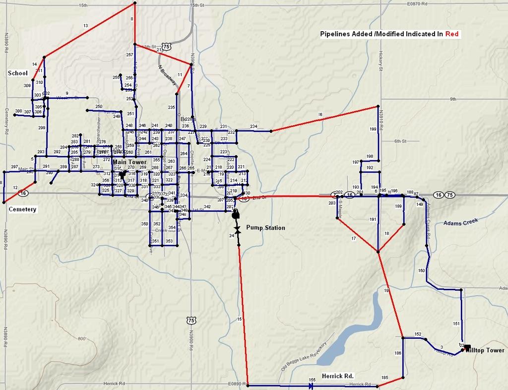
90 82