Appendix B: Analysis Worksheets

Transcription

1 Appendix B: Analysis Worksheets

2 Table of Contents Candidate Cause 1: High Flows... 4 Worksheets: 1, 2, 4, and Candidate Cause 2: Intraspecific Competition Worksheet: Candidate Cause 3: Interspecific Competition Worksheet: Candidate Cause 4: YOY Food Quality Worksheets: 24 and Candidate Cause 5: Egg Quality Worksheet: Candidate Cause 6: YOY Habitat Worksheets: 34, 35 and Candidate Cause 7: Temperature Worksheets: 7, 8, 9, 10, 11, and Candidate Cause 8: ph Worksheets: 13 and Candidate Cause 9: Dissolved Oxygen (DO) Worksheets: 18, 19, 23, Candidate Cause 10: Ammonia (NH 3 ) Worksheets: 20, 21 22, and Candidate Cause 11: Algal and Bacterial Toxins Worksheets: 15, 16, 17, 32, 33, and Candidate Cause 12: Toxic Chemicals Worksheets: 37.1, 38, 39, 40, 42, 44, 45, and Candidate Cause 13: EDCs Worksheets: 43, 47, 48, and Candidate Cause 14: Pathogens and Parasites Worksheets: 27, 29, 30, and Worksheets not used as Evidence in the CADDIS Decision Process Worksheets: 41, 43, and i

3 Below is a list of all the analysis worksheets contained in this appendix. Worksheet Worksheet Title Number 1 Temporal Co-occurrence of Flow 2 Smallmouth Bass Abundance and Stream Discharge (Q) 3 Stressor-Response Relationships of Small Mouth Bass 4 Effects of previous year mean June discharge and previous year YOY CPUE on SMB age-1 CPUE 5 Analysis of Fish Communities in the Susquehanna River Basin 6 Stream Discharge (Q) and Small Mouth Bass Spawning 7 Continuous data from SRBC Early Warning System Dataset for Rockville site 8 Continuous data from SRBC Early Warning System Dataset for Danville site 9 Continuous data from SRBC Early Warning System Dataset for Columbia site 10 Intra and inter site comparison of water temperature using Data from the Case 11 Temperature Criteria of Small Mouth Bass 12 Impacts of High Temperatures on YOY 13 Impacts of High ph on Small Mouth Bass Survival 14 Increases in ph on the Susquehanna River, Major Tributaries and Out-of-Basin Increases in Dissolved Organic Phosphorus in the Susquehanna River: Hypothesizing an Increase in OrthoP within the Juniata/Lower Susquehanna Subbasins Hypothesizing an increase in Total Phosphorus within the Juniata/ Lower Susquehanna Subbasins 18 Impacts of Low Dissolved Oxygen on Small Mouth Bass Survival and Recruitment 19 Impacts of Low Dissolved Oxygen on Small Mouth Bass Survival 20 Impacts of Ammonia toxicity on the survival and recruitment of Small Mouth Bass 21 Toxicity of Ammonia to Early Life Stages of Smallmouth Bass 22 Hypothesizing an increase in NH3 within the Juniata/Lower Susquehanna Subbasins 23 Extreme Discharge (Q) Events and Increases in Ortho-P Trends Apparent decline in Susquehanna Smallmouth bass (SMB) and increase in the Non-native Rusty Crayfish Impacts of decreased food quality on YOY Small Mouth Bass and on Adults susceptibility to disease 26 Impacts of decreased food quality on Small Mouth Bass Eggs 27 YOY Smallmouth Bass and Abiotic Factors 29 Impacts of Pathogens (LMBV) or Parasites on Small Mouth Bass Populations 30 Impacts of Pathogens and Parasites on YOY Smallmouth Bass 31 Disease Prevalence in YOY Small Mouth Bass 32 Cyanobacteria and potential cyanotoxin producing taxa collected from sites corresponding to the 2014 adult small mouth bass liver tissue toxicology tests 33 Spatial comparison of Microcystin levels in smallmouth bass liver tissue 34 Impacts of algal blooms on YOY Smallmouth Bass 35 Algal and Cyanobacterial Toxins 36 Decreases in late summer YOY habitat as a result of reduced late summer flows and YOY Mortality 37 Passive Sampler and Sediment Results Maps; Data 38 Historical Pesticides/PCB s in Sediment 39 Historical Pesticides (PCBs) 2

4 40 Metals in Sediment 41 Chemical Compounds in the Susquehanna River Basin 42 Chemical Compounds in the Susquehanna River Basin 43 Hormones Analyzed from Passive Water Samplers 44 WQN Pesticides 45 Marietta Metals vs. Upstream Sites November 2013 Analysis 46 Grab Metal Samples 47 Hormones in Sediments 48 EDCs and Intersex in Adult SMB 49 Total Estrogenicity 50 Nutrients and Cyanobacteria 51 Low Dissolved Oxygen and Decreasing Small Mouth Bass Survival and Recruitment 52 Ammonia Toxicity and Decreasing Small Mouth Bass and Recruitment 54 Stroud Study Temperature Cycling and Maximum Temperature Effects on SMB 3

5 Candidate Cause 1: High Flows Worksheets: 1, 2, 4, and 6 4

6 Title: Temporal Co-occurrence of Flow (WS #1) Agency: Pennsylvania Department of Environmental Protection Temporal Co-occurrence using Data from the Case Candidate Cause: Increased frequency of high spring discharge and low summer discharge. Introduction: Stressful discharge conditions for smallmouth bass (SMB) young of year (YOY) can be two fold. High discharges during spring can remove fry from their habitat and summer low discharges can cause stress to the point where YOY survival is decreased or YOY are more likely to become prey. Both situations can increase mortality and decrease recruitment to age class 1+. If spring high discharges or summer low discharges were the cause of decreased recruitment to age class 1+ observed post-2002, then we would expect to see higher discharges in spring or lower discharges in summer. Data: The Pennsylvania Department of Environmental Protection (PA DEP) obtained hourly discharge data from the Harrisburg USGS gage station for water-years 1990 to Analysis and results: Discharge data were summarized into seasonal daily durations that were 50,000 CFS (for spring) and 5,000 CFS (for summer) using AQUARIUS software. These thresholds characterized the upper 75 th percentile and lower 25 th percentile of the entire dataset, respectively. The spring time period was defined as discharge from the beginning of March to the end of June, and the summer time period was defined as discharge from the beginning of July to the end of September. Datasets were then qualified as either pre-2002 or post-2002 for comparison purposes. The resulting seasonal datasets were analyzed using R software. Daily spring high discharges were normally distributed; therefore, time period differences were evaluated using ANOVA. However, daily summer low discharges did not exhibit acceptable normal distribution; consequently, Kruskal-Wallis test was used. There was no significant difference between pre and post-2002 spring high discharges (p = 0.98). Pre and post-2002 spring high discharges were surprisingly similar, averaging 26.5 days per year and 26.6 days per year, respectively (Figure 1). There was also no significant difference between pre and post-2002 summer low discharges (p = 0.06). Although summer low discharges were not statically different, it was 5

7 interesting to see that pre-2002 summer low discharges had longer durations and were more frequent (year by year) than post-2002 (Figure 2). Figure 1. The number of spring days per year where discharge exceeded 50,000 CFS. Trend lines were added for qualitative purposes only. 6

8 Figure 2. The number of summer days per year where discharge was at or below 5,000 CFS. Trend lines were added for qualitative purposes only. Conclusion: The evidence weakens the argument for increased frequency of high spring flow and low summer discharge as the cause of the low recruitment of Age1+ SMB. 7

9 Title: Smallmouth Bass Abundance and Stream Discharge (Q) (WS #2) Agency: Environmental Protection Agency Stressor-Response Relationships Candidate Cause: Decreased abundance of YOY SMB because of stream discharge Introduction: The temporal pattern of streamflow fluctuation appears to be the most important abiotic factor determining nesting success and failure of SMB in perennial streams (Lukas and Orth 1995). Increased stream discharge increases water velocity which can result in mechanical nest failure or dislodge young fry from their habitat, increasing mortality and decreasing survival and subsequent recruitment. Nesting success during a stable low flow year was 73% whereas nesting success was only 35% during a year with heavy precipitation in a Tennessee Stream (Reynolds and O Bara 1991). Similarly, Buynak and Mitchell (2002) found that year-class strength of SMB in Elkhorn Creek (KY) was inversely related to April-July rainfall totals. In the South Anna River (VA), most nest failures were directly attributable to flows (Lukas and Orth 1995). In three other Virginia rivers, Smith et al. (2005) found that mean June stream discharge most consistently related to age-0 CPUE. Similarly, in Pennsylvania rivers, low river discharge during select spring periods tends to lead to above average YOY catch rates (Lorantas and Kristine 2004). However, below average catch rates of YOY SMB in recent years and reductions in catch rates of all sizes of SMB and SMB 300mm in the Susquehanna River relative to reference periods have been uncharacteristic of changes evident in other rivers across the state (Lorantas et al. 2012). The intent of this comparison is to assess the relationship between YOY SMB abundance and stream discharge and determine whether there have been temporal and/or spatial changes in the relationship. Specifically, If stream discharge were influencing abundance, we would expect to see (1) a strong negative relationship between the two variables; (2) the negative relationship would be as strong or stronger at the subject sites and time periods than at the comparison sites and time periods; and (3) recent YOY CPUE (i.e., from 2005 to present) would fall within the prediction limits calculated based on the historical (i.e., comparison time period) relationship between YOY CPUE and stream discharge. 8

10 Data: Back-pack electrofishing catch per unit effort (CPUE; fish/ 50 m) data for YOY SMB from PFBC s state-wide monitoring network was included in the analysis. Site-specific CPUE data were aggregated by river reach and by year. Mean June stream discharge data (Q) was obtained from U.S. Geological Survey, USGS Surface-Water Monthly Statistics for the Nation application. Values were generated for representative stream gaging locations for each reach of river used in the analysis. These included Susquehanna River at Harrisburg ( ) and Danville ( ), Delaware River at Trenton ( ), Juniata River at Newport ( ) and Mapleton Depot ( ), West Branch Susquehanna River at Lewisburg ( ), and Allegheny River at Franklin ( ). Analysis and results: Spearman Rank correlation were conducted for YOY CPUE and mean June Q (suggest by Smith et al. 2005) values for each of the subject and comparison locations for the and time periods to assess the relationship between the two variables for the two time periods. Relationships between YOY CPUE weakened during the time period compared to the time period for all subject reaches while the same relationships at comparison site strengthened (Table 1). The relationship between June Mean flows and YOY CPUE was plotted for the comparison period from 1990 to The relationship between mean June flow (on the X-Axis) and YOY CPUE (on the Y-Axis) was modelled using linear regression after log- transforming flow. The regression line and prediction limits were back-transformed to produce the plots shown (Figures 1-8). YOY CPUE and flow data from the pre-2005 and post-2005 periods are plotted on the same figures. Post-2005 data for both case reaches (lower Juniata River and middle Susquehanna River) largely fall near or below the prediction limits based on discharge (Figures 2 and 4) while post-2005 data from comparison reaches (upper Juniata River, upper Susquehanna River, lower Susquehanna River, West Branch Susquehanna River, upper Allegheny River, and lower Delaware River) fall near or within prediction limits based on discharge (Figures 1,3,5-8). Conclusion: For the subject sites, the relationship between YOY SMB abundance and flow has weakened for the post-2005 period while this relationship has strengthened in comparison reaches for the post-2005 period. Further, reach-specific linear regression models of YOY SMB catch rates based stream discharge demonstrated that post

11 catch rates of YOY SMB frequently fell outside of prediction bounds set by the models. Previous analysis by Lorantas et al. (2012) to develop recruitment models to predict future age class abundance also identified discrepancies in predicted results for portions of the Susquehanna Basin. These analyses suggest the decrease YOY SMB catch rates in subject reaches is not being completely driven by natural factors that typically control YOY SMB mortality. Regression analysis suggests that while high stream discharges in June still negatively affects YOY SMB abundance, other factors are affecting abundance within subject reaches during years with low stream discharge in June. Literature Cited: Buynak, G.L., & B. Mitchell Response of Smallmouth Bass to regulatory and environmental changes in Elkhorn Creek, Kentucky. North American Journal of Fisheries Management 22: Lorantas, R.M., & D.P. Kristine Annual monitoring of young-of-year abundanceof Smallmouth Bass in rivers in Pennsylvania; relationships between abundance, river characteristics, and spring fishing. Pennsylvania Fish and Boat Commission, Bureau of Fisheries, Fisheries Management Division, Bellefonte, Pennsylvania. Lorantas, R., T. Wagner, D. Arnold, J. Detar, M. Kaufmann, K. Kuhn, R. Lorson, R. Wnuk, & A. Woomer Smallmouth Bass electrofishing catch rate in large Pennsylvania rivers and examination of Smallmouth Bass recruitment indices. Pennsylvania Fish and Boat Commission, Bureau of Fisheries, Fisheries Management Division, Bellefonte, Pennsylvania. Lukas, J.A., & D.J. Orth Factors affecting nesting success of Smallmouth Bass in a regulated Virginia stream. Transactions of the American Fisheries Society 124: Reynolds, C.R., & C.J. O Bara Reproductive ecology and spawning habitat of Smallmouth Bass in two small streams of the Tennessee River system. Pages in D.C. Jackson, editor. Proceedings of the First International Smallmouth Bass Symposium. Mississippi Agricultural and Forestry Experiment Station, Mississippi State University, Starkville, Mississippi. 10

12 Table 1: Spearman Rank correlation of reach-wide YOY SMB catch per unit effort (CPUE; fish/ 50 m) and mean June discharge (Q) at large river reaches in Pennsylvania. Results are broken into pre-2005 and post-2005 time periods. Direction values (weakening (-), substantial weakening (--), and strengthing (+)) comment on the changes in the relationship between the values from the pre-2005 period to the post period. Spearman's rank correlation rho (YOY SMB cpue: mean June Q) Reach x y S p rho status direction upper Juniata River lower Juniata River ujprec ljprec ujpreq ljpreq E comparison subject ujpostc ljpostc ujpostq ljpostq comparison subject - -- upper Susquehanna usprec uspreq comparison River uspostc uspostq comparison + middle Susquehanna msprec mspreq 864 <2.2e subject River mspostc mspostq subject - lower Susquehanna lsprec lspreq subject River lspostc lspostq subject - West Branch WBpreC WBpreQ comparison Susquehanna River WBpostC WBpostQ comparison + uaprec uapreq comparison upper Allegheny River uapostc uapostq comparison + lower Delaware River LDpreC LDpreQ comparison LDpostC LDpostQ comparison + 11

13 Figure 1. Linear regression model of YOY SMB catch per unit effort (CPUE; fish/ 50 m) and mean June discharge (Q; cubic meters per second) at the upper Juniata River for the period Regression lines, confidence limits, prediction limits are from back transformed log discharge values. Black dots indicate YOY CPUE values for pre period and red dots indicate CPUE values for post-2005 period. Figure 2. Linear regression model of young-of-year YOY SMB catch per unit effort (CPUE; fish/ 50 m) and mean June discharge (Q; cubic meters per second) at the lower Juniata River for the period Regression lines, confidence limits, prediction limits are from back transformed log discharge values. Black dots indicate YOY CPUE values for pre-2005 period and red dots indicate CPUE values for post-2005 period. 12

14 Figure 3. Linear regression model of YOY SMB catch per unit effort (CPUE; fish/ 50 m) and mean June discharge (Q; cubic meters per second) at the upper Susquehanna River for the period Regression lines, confidence limits, prediction limits are from back transformed log discharge values. Black dots indicate YOY CPUE values for pre-2005 period and red dots indicate CPUE values for post-2005 period. Figure 4. Linear regression model of young-of-year YOY SMB catch per unit effort (CPUE; fish/ 50 m) and mean June discharge (Q; cubic meters per second) at the middle Susquehanna River for the period Regression lines, confidence limits, prediction limits are from back transformed log discharge values. Black dots indicate YOY CPUE values for pre-2005 period and red dots indicate CPUE values for post-2005 period. 13

15 Figure 5. Linear regression model of YOY SMB catch per unit effort (CPUE; fish/ 50 m) and mean June discharge (Q; cubic meters per second) at the lower Susquehanna River for the period Regression lines, confidence limits, prediction limits are from back transformed log discharge values. Black dots indicate YOY CPUE values for pre-2005 period and red dots indicate CPUE values for post-2005 period. Figure 6. Linear regression model of YOY SMB catch per unit effort (CPUE; fish/ 50 m) and mean June discharge (Q; cubic meters per second) at the West Branch Susquehanna River for the period Regression lines, confidence limits, prediction limits are from back transformed log discharge values. Black dots indicate YOY CPUE values for pre-2005 period and red dots indicate CPUE values for post period. 14

16 Figure 7. Linear regression model of YOY SMB catch per unit effort (CPUE; fish/ 50 m) and mean June discharge (Q; cubic meters per second) at the upper Allegheny River for the period Regression lines, confidence limits, prediction limits are from back transformed log discharge values. Black dots indicate YOY CPUE values for pre-2005 period and red dots indicate CPUE values for post-2005 period. 15

17 Figure 8. Linear regression model of YOY SMB catch per unit effort (CPUE; fish/ 50 m) and mean June discharge (Q; cubic meters per second) at the lower Delaware River for the period Regression lines, confidence limits, prediction limits are from back transformed log discharge values. Black dots indicate YOY CPUE values for pre period and red dots indicate CPUE values for post-2005 period. 16

18 Title: Effects of previous year mean June discharge and previous year YOY CPUE on SMB age-1 CPUE (WS #4) Agency: Pennsylvania Fish and Boat Commission Stressor-Response Relationships Candidate Cause: Decreased abundance of YOY SMB because of stream discharge. Introduction: Fish recruitment is typically defined as the number of fish that survive to a specific age or size in a given year. Although recruitment can be defined in a number of ways, it is most commonly specified as either the number of fish that reach age 1 each year or the number of fish that survive to the first age they can be captured in the fishery. In most cases fish are considered recruited to the population after they reach a size or age at which very high larval mortality rates have already occurred and the fish can be considered part of the adult population (Allen and Hightower 2010). This analysis will focus on two associated variables (previous year mean June discharge and previous year YOY CPUE) and their influence on age-1 CPUE during adult SMB surveys. The intent of the analysis is to evaluate whether there have been changes in relationship of river flow the previous year, which strongly drives YOY SMB abundance, and age-1 CPUE. Also, whether there have been changes in the relationship between YOY SMB CPUE and age-1 CPUE. Comparison of these variables with age-1 CPUE would help to account for changes in survival between age- 0 (YOY) and age-1 SMB during the pre-2005 and post-2005 period. Varying levels of mortality from age 0 to age 1 would have occurred in these SMB populations historically (e.g., predation, over-winter mortality); however, more recent events may have changed this dynamic. Temporal changes in these relationships would suggest that factors dictating recruitment of SMB from age 0 to age 1 (and the adult population) have changed between the two periods of time. As with YOY SMB CPUE and mean June discharge, you would expect a negative relationship when comparing age-1 CPUE and mean June discharge the previous year. Several other factors will contribute to the survival of SMB from age 0 to age 1 so the relationship should be weaker than the YOY SMB CPUE and mean June discharge relationship; however, the directionality should be similar. The relationship between age-1 CPUE and the previous year YOY CPUE should be positive (i.e., the higher abundance YOY SMB leads to the higher abundance of age-1 SMB the following year). Data: Boat electrofishing catch per unit effort (CPUE; fish/h) data of age-1 SMB from Pennsylvania Fish and Boat Commission (PFBC) state-wide monitoring network was 17

19 included in the analysis. Age-1 catch was estimated using an age-length key based on a stratified, random sample of aged adult SMB for each site. Cumulative age-1 catch and cumulative effort were calculated for each reach for each year and applied to generate age-1 CPUE values. Backpack electrofishing CPUE (fish/ 50m) data for YOY SMB data from PFBC state-wide monitoring network was also included in the analysis. Site-specific CPUE data were aggregated by river reach and by year. Mean June stream discharge data (Q) was obtained from U.S. Geological Survey, USGS Surface-Water Monthly Statistics for the Nation application. Values were generated for representative stream gaging locations for each reach of river used in the analysis. These included Susquehanna River at Harrisburg ( ) and Danville ( ), Delaware River at Trenton ( ), Juniata River at Newport ( ) and Mapleton Depot ( ), West Branch Susquehanna River at Lewisburg ( ), and Allegheny River at Franklin ( ). Discharge values used were for the year the fish would have been spawned (i.e., 2008 CPUE would relate to mean June Q during 2007). Analysis and results: Spearman Rank correlation were conducted for age-1 SMB CPUE and mean June Q values for the previous year for each of the case and comparison locations for the and time periods to assess relationship between the two variables for the two time periods. Relationships between age-1 CPUE and previous year s mean June discharge substantially weakened during the time period compared to the time period for the upper Juniata River (comparison), lower Juniata River (case), and middle Susquehanna River (case); weakened at the upper Susquehanna River (comparison); and substantially strengthened at the upper Allegheny River (comparison) (Table 1). Spearman Rank correlation were conducted for age-1 SMB CPUE and previous year YOY SMB CPUE for each of the subject and comparison locations for the and time periods to assess relationship between the two variables for the two time periods. Relationships between age-1 CPUE and previous year s YOY SMB CPUE substantially weakened during the time period compared to the time period for the upper Juniata River (comparison), lower Juniata River (case), and middle Susquehanna River (case); weakened at the upper Susquehanna River (comparison); and substantially strengthened at the upper Allegheny River (comparison) (Table 1). The relationship between previous year s June Mean flows and age-1 SMB CPUE was plotted for the comparison period from 1990 to The relationship between mean June flow (on the X-Axis) and YOY CPUE (on the Y-Axis) was modelled using linear 18

20 regression after log- transforming flow. The regression line and prediction limits were back-transformed to produce the plot shown to the right. YOY CPUE and flow data from the post 2005 period were then plotted on the same figure. The data for the subject reaches(figures 2 and 4) plotted largely at or near the lower prediction limit while comparison reaches were more widely distributed within the prediction limits (Figures 1, 3, and 5). The only exception being the West Branch Susquehanna River (Figure 6) where the predicted distribution of the post-2005 results is similar to those of the subject reaches. Conclusion: For the case sites, the relationship between age-1 YOY SMB CPUE and previous year mean June flow and previous year YOY SMB CPUE has weakened in the near term for subject sites. For comparison sites, the relationship between YOY abundance and flow has strengthened for the post-2005 period. It is likely that flow is not the major factor in the subject areas. A decrease in abundance is not being completely driven by natural factors controlling YOY mortality, although there may be some component of it that is. Literature Cited: Allen, M.S., & J.E. Hightower Fish population dynamics: mortality, growth, and recruitment. Pages in W.A. Hubert and M.C. Quist, editors. Inland fisheries management in North America, 3 rd edition. American Fisheries Society, Bethesda, Maryland. Table 1: Spearman Rank correlation of reach-wide Age-1 SMB catch per unit effort (CPUE; fish/ 50 m) and previous year s mean June discharge (Q) at large river reaches in Pennsylvania. Results are broken into pre-2005 and post-2005 time periods. Direction values (weakening (-), substantial weakening (--), and substantial strengthening (++)) comment on the changes in the relationship between the values from the pre-2005 period to the post-2005 period. 19

21 Reach x y S p rho status direction upper Juniata River lower Juniata River upper Susquehanna River middle Susquehanna River upper Allegheny River ujprec ujpreq comparison ujpostc ujpostq comparison -- ljprec ljpreq subject ljpostc ljpostq subject -- usprec uspreq comparison uspostc uspostq comparison - msprec mspreq subject mspostc mspostq subject -- UApreC UApreQ comparison UApostC UApostQ comparison ++ Table 2: Spearman Rank correlation of reach-wide Age-1 SMB catch per unit effort (CPUE; fish/ 50 m) and previous year s YOY Smallmouth Bass catch per unit effort (CPUE; fish/ 50 m) at large river reaches in Pennsylvania. Results are broken into pre and post-2005 time periods. Direction values (weakening (-), substantial weakening (--), and strengthening (+)) comment on the changes in the relationship between the values from the pre-2005 period to the post-2005 period. Reach x y S p rho status direction upper Juniata River lower Juniata River ujprec ljprec ujpreq ljpreq comparison subject ujpostc ljpostc ujpostq ljpostq comparison subject - -- upper Susquehanna usprec uspreq comparison River uspostc uspostq comparison + middle Susquehanna msprec mspreq subject River mspostc mspostq subject -- lower Susquehanna lsprec lspreq comparison River lspostc lspostq comparison - West Branch WBpreC WBpreQ comparison Susquehanna River WBpostC WBpostQ comparison - uaprec uapreq comparison upper Allegheny River uapostc uapostq comparison + 20

22 Figure 1: Linear regression model of age-1 SMB catch per unit effort (CPUE; fish/ 50 m) and previous year mean June discharge (Q; cubic meters per second) at the upper Juniata River for the period Regression lines, confidence limits, prediction limits are from back transformed log discharge values. Black dots indicate YOY CPUE values for pre-2005 period and red dots indicate CPUE values for post-2005 period Figure 2: Linear regression model of age-1 SMB catch per unit effort (CPUE; fish/ 50 m) and previous year mean June discharge (Q; cubic meters per second) at the lower Juniata River for the period Regression lines, confidence limits, prediction limits are from back transformed log discharge values. Black dots indicate YOY CPUE values for pre-2005 period and red dots indicate CPUE values for post-2005 period 21

23 Figure 3: Linear regression model of age-1 SMB catch per unit effort (CPUE; fish/ 50 m) and previous year mean June discharge (Q; cubic meters per second) at the upper Susquehanna River for the period Regression lines, confidence limits, prediction limits are from back transformed log discharge values. Black dots indicate YOY CPUE values for pre-2005 period and red dots indicate CPUE values for post period Figure 4: Linear regression model of age-1 SMB catch per unit effort (CPUE; fish/ 50 m) and previous year mean June discharge (Q; cubic meters per second) at the middle Susquehanna River for the period Regression lines, confidence limits, prediction limits are from back transformed log discharge values. Black dots indicate YOY CPUE values for pre-2005 period and red dots indicate CPUE values for post period 22

24 Figure 5: Linear regression model of age-1 SMB catch per unit effort (CPUE; fish/ 50 m) and previous year mean June discharge (Q; cubic meters per second) at the lower Susquehanna River for the period Regression lines, confidence limits, prediction limits are from back transformed log discharge values. Black dots indicate YOY CPUE values for pre-2005 period and red dots indicate CPUE values for post period Figure 6: Linear regression model of age-1 SMB catch per unit effort (CPUE; fish/ 50 m) and previous year mean June discharge (Q; cubic meters per second) at the West Branch Susquehanna River for the period Regression lines, confidence limits, prediction limits are from back transformed log discharge values. Black dots indicate YOY CPUE values for pre-2005 period and red dots indicate CPUE values for post-2005 period 23

25 Title: Stream Discharge (Q) and Smallmouth Bass Spawning (WS #6) Agency: Pennsylvania Department of Environmental Protection Temporal Co-occurrence using Data from the Case Candidate Cause: Limiting water quality conditions, elevated contaminant loads or other candidate causes that may be impacting YOY SMB vs. temporal development of SMB. Introduction: The candidate cause analyses characterized to specifically affect SMB YOY should consider when the data was collected in any given year in order to validate that SMB were obligated to a specific habitat from which the data may have been collected. SMB YOY may only be vulnerable to specific constituents or conditions in near-shore habitats for a short period each spring. And on any given year that period could shift due to warmer/colder than normal temperatures or could be interrupted due to, among other conditions, elevated flow events. Data: DEP Water Quality Standards staff performed a literature review of the early life history of SMB in an attempt to create a hypothetical timeline that could promote temporal context of data analyses. This temporal context could be used to determine the potential stage of YOY development when particular conditions or exposure(s) and if YOY were physically obligated to a particular habitat. In addition continuous instream monitoring data collected by USGS New Cumberland for Juniata River at Newport (main channel) and Howe Twp. (micro habitat) and the Susquehanna River at Clemson Island (main channel and micro habitat) for 2008 & 2009 were plotted to compare to life history information. Analysis and Results: When the littoral water temperature approaches 13 C - 15 C, male SMB migrate to the littoral zone of lakes and rivers to build nests. Once nests are built, spawning may occur at temperatures ranging from 12.8 C C but typically occurs at 16 C (Ridgway 1988, Armour 1993, Scott 1993). Sudden drops in temperature below 14 C are lethal to the embryos and may also result in the male abandoning the nest (MacLean et al. 1981, Armour 1983). Eggs hatch 2-10 days after deposition and the hatchlings or wrigglers are at first clear in color and absorb nutrients from their yolk sacs. They remain on the bottom of the nest and within days develop a black pigmentation. The black-fry are mm in length 24

26 during this time and remain on the nest for 3-11 days before rising (Beeman 1924; Shuter et al. 1980; Scott and Crossman 1973). Larvae are mm total length at the time of swim-up from a nest (Vogel 1981, Shuter et al. 1980), and grow about 1 mm/d over the following 30 d (Scott and Crossman 1973, Carlander 1977, Becker 1983). After rising they remain in a dense mass close to the bottom of the nest and within two days they begin to disband. Seven to nine days after rising from the nest, they metamorphose into typical SMB (Ridgway 1988). During this time habitat use is dictated by the movement of the male. The male prevents the young from straying too far and patrols the area for predators (Ridgway 1988, Sabo and Orth 1994). As the YOY grow, they begin feeding on larger invertebrate prey (Sabo and Orth 1994), male defense declines (Ridgway 1988) and they begin to disperse further and further from the nest site during the day. They continue to aggregate into dense schools above the nest at night (Wales 1981). Once the fry are mm in length, the male reduces parental care and eventually abandons the nest (Ridgway and Friesen 1992). Desertion coincides with the dispersal of the fry from the nest site and the infiltration of new microhabitats. Two to four weeks after dispersal the YOY move in small schools to shallower waters than their nest sites but remain within 200 m of the nest. They show a preference for boulder and rock habitats, possibly to avoid predation (Serns 1982, Houpt 1991, Sabo and Orth 1994). Temperatures during the first summer growing season are positively correlated with year class strength. This relationship exists because energy reserves which the young use to survive their first winter are produced in the summer when food is abundant and the water temperature is most suitable for growth (Horning and Pearson 1973, Clady 1975, Shuter et al. 1980). Analysis/Continuous Instream Monitoring (CIM) Data: Continuous temperature, ph and dissolved oxygen data from near-shore/micro-habitats were plotted together on charts to determine the potential sequence of events for smallmouth bass pre- through post-spawn and YOY dispersal. 25

27 Results: Figure Water temperature at Howe Twp (main channel and micro habitat) and Clemson (main channel and micro habitat) vs. discharge. 26

28 Figure Water temperature at and Clemson (main channel and micro habitat) vs. discharge. 27

29 In 2008 water temperatures at all Howe Twp. and Clemson Island sites exceeded and maintained temperatures above 16 C on/after May 26 th and should have initiated SMB spawning. Discharge after May 26 th consistently decreased with little evidence of major elevated discharge events that would have resulted in an unsuccessful spawn (Figure 1). Nests and eggs could have been exposed to sediment contamination or near-shore water column contamination from about May 26 th for as long as about 10 days (June 6 th ). Discharge for at least the next 35 days was stable and YOY SMB may have dispersed from near-shore/micro habitats approximately July 1 st July 11 th. A review of when PFBC YOY were collected and YOY length data could be consulted to verify this hypothetical timeline. In 2009 water temperature at Clemson Island exceeded and maintained temperatures above 16 C on/after May 19 th and should have initiated SMB spawning. Discharge steadily decreased for approximately 9 days, which may have been enough time for eggs to hatch. After 10 days a major flow event occurred, which would have impacted those fish that had successfully spawned. As of June 2 nd flows had decreased and a 2 nd spawn could have occurred. After a maximum of 10 days (June 12 th ), eggs could have hatched. Another major flow event occurred on June 19 th, which could have again disrupted a successful spawn for many, but given the 7-day period there may have been just enough opportunity for swim-up to occur (Figure 2). Nests and eggs could have been exposed to sediment contamination or near-shore water column contamination for two periods (May 19 th May 28 th and June 2 nd June 12 th ). Conclusion: Discharge and water temperature variability in any given year/season could dictate the magnitude of affect from a candidate cause and could help explain the variability of YOY disease and maybe SMB recruitment at sites from year to year. 28

30 Candidate Cause 2: Intraspecific Competition Worksheet: 3 29

31 Title: Stressor-Response Relationships of Smallmouth Bass (WS #3) Agency: Pennsylvania Fish and Boat Commission Candidate Cause: Intraspecific competition resulting from density-dependent factors associated with populations at or above carrying capacity negatively impacted the condition of SMB and resulted in increased susceptibility to disease and mortality. Introduction: Condition indices offer fishery scientists a tool to evaluate the effects of various management strategies and, indirectly, ecological interactions in fish populations and communities (Murphy and Willis 1991). When combined with other information including density, condition data provide fishery scientists a more complex understanding of population dynamics (recruitment, growth, and mortality) and environmental influences (Pope and Kruse 2007). Wege and Anderson (1978) proposed the use of relative weight (W r ) to evaluate fish condition. W r is a comparison of the weight of fish in a population to the standard weight (W s ) for that species. Standard weight is a lengthderived estimate of weight of a fish based on length-weight regressions from a number of different populations. Kolander et al. (1993) developed the standard weight equation for SMB from 50 populations from 19 states, including populations from the Susquehanna and Juniata rivers. W r of fish in a population as a whole or in different components of the population (total length groups in this instance) vary with resource availability. When W r values are well below 100 for an individual or a component of the population, problems may exist in food or feeding conditions; when W r values are well above 100, fish may not be making the best use of surplus prey (Anderson and Neumann 1996). A population or subpopulation with an average relative weight less than 80 is likely resource limited (Pope et al. 2010). The intent of this analysis was to evaluate W r in subject reaches between the pre-2005 and post-2005 periods and among comparison reaches over the same time periods; looking for broad shifts in condition that may indicate resource limitations resulting from, at least in part, intraspecific competition. Specifically, if intraspecific competition were influencing abundance, we would expect to see (1) pre-2005 W r values at subject reaches near or below 80; (2) a marked increase in condition at subject reaches during the post-2005 period; and (3) W r values at subject sites would be different than those at comparison sites during the same periods. Data: Data used for analysis included individual SMB length and weight data from riverine populations across the Commonwealth collected by Pennsylvania Fish and Boat Commission (PFBC) during boat electrofishing surveys. Data were aggregated by river- 30

32 reach to increase sample sizes. Only post-1990 data were included as that was the time period when consistent length-weight data was available for case reaches (middle Susquehanna River and lower Juniata River). Analysis and Results: Relative weight values were generated using a revision of the standard weight equation for SMB (Kolander et al. 1993). W r values were generated for all adult SMB with individual length and weight data from each river reach. Data were grouped into 25 mm total length (TL) bins by year to assess whether changes were specific to different sizes of fish within the population. Only fish greater than 150 mm TL were included in the analysis as suggested by Kolander et al. (1993). Mean W r per TL group per year (error bars indicate ± standard deviation) was calculated and plotted graphically to assess whether temporal shifts during the study period occurred. Results varied by TL bin and by year for each of the river reaches included in the analysis. Temporal comparisons of W r at the middle Susquehanna River (Figure 1) and lower Juniata River (Figure 2) demonstrate that W r during the study period was at or near the 100 benchmark for nearly all TL bins, indicating good fish condition, overall. W r values at the middle Susquehanna River were similar to those at the Allegheny River (Figure 3) and the upper Susquehanna River (Figure 4) during the study period. W r values at the Delaware River (Figure 5) were generally lower than those of the middle Susquehanna River during the study period. W r values at the West Branch Susquehanna River were generally lower, especially for larger TL groups, than at the middle Susquehanna River for most of the study period (Figure 6). Lower Juniata River W r values where similar to those at the upper Juniata River (Figure 7) during the study period. Conclusion: The relative weight (W r ) data from the middle Susquehanna River and lower Juniata River suggest that fish condition during the pre-2005 period was not especially low as a result of intraspecific competition. If the abundance of adult SMB during the pre-2005 period had exceeded the carry capacity, it would have resulted in reduced condition at the subject reaches in temporal comparisons (pre-2005 and post-2005). The mean W r data for the subject reaches is similar between periods despite decreases in abundance of Smallmouth Bass in the post-2005 period. Additionally, mean W r at subject reaches was similar to comparison reaches through the time period. This suggests that conditions within subject reaches were not appreciably different than those encountered in comparison reaches during the same time frame. 31

33 32

34 33

35 34

36 35

37 36

38 37

39 Literature Cited: Anderson, R.O., & R.M. Neumann Length, weight, and associated structural indices. Pages in B.R. Murphy and D.W. Willis, editors. Fisheries Techniques, 2nd Edition. American Fisheries Society, Bethesda, Maryland. Kolander, T.D., D.W. Willis, & B.R. Murphy Proposed revision of the standard weight (W s ) equation for Smallmouth Bass. North American Journal of Fisheries Management. 13: Pope, K.L., & C.G. Kruse Condition. Pages in C.S Guy and M.L. Brown, editors. Analysis and interpretation of freshwater fisheries data. American Fisheries Society, Bethesda, Maryland. Pope, K.L., S.E. Lochman, & M.K. Young Methods for assessing fish populations. Pages in W.A. Hubert and M.C. Quist, editors. Inland fisheries management in North America, 3 rd edition. American Fisheries Society, Bethesda, Maryland. 38

40 Murphy, B.R., & D.W. Willis Application of relative weight (W r ) to western warmwater fisheries. Pages in J.L. Cooper and R.H. Hamre, editors. Warmwater fisheries symposium I. U.S. Forest Service General Technical Report RM-207, Fort Collins, Colorado. Wege, G.J., & R.O. Anderson Relative weight (W r ): a new index of condition for Largemouth Bass. Pages in G. Novinger and J. Dillard, editors. New approaches to the management of small impoundments. American Fisheries Society, North Central Division, Special Publication 5, Bethesda, Maryland. 39

41 Candidate Cause 3: Interspecific Competition Worksheet: 5 40

42 Title: Analysis of Fish Communities in the Susquehanna River Basin (WS #5) Agency: Pennsylvania Department of Environmental Protection Candidate cause: Increased non-native species decrease Smallmouth Bass recruitment, Age 1+ Introduction: The structure and function of a fish community is regulated by multiple biotic and abiotic factors. The most influential of the biotic factors are typically thought to be predation and competition (Sih et al. 1985, Persson, 1988). Interspecific competition, hereafter referred to simply as competition, occurs when individuals from different species compete over the same resources (Larkin 1956, MacArthur and Levins 1967, Abrams 1983). The introduction and spread of aquatic invasive species can have multiple effects on ecosystems and can lead to habitat degradation, loss of native flora and fauna (D Antonio 2001, King 1984, Arim et al. 2006) and disease vectoring and proliferation (Andow et al.1990). Invasive species have been identified as the second leading cause, next to habitat degradation, of imperiled fishes in the United States (Wilcove et al.1998) and this conclusion is similar worldwide (Clavero and Garcia-Berthou 2005). The rapid density increases brought about by the exponential growth rates of an invasive species (Arim et al. 2006) provide the pathway for increased competition with native fauna. This competition with invasive species has been identified as a major source, albeit not the only pathway, for native species declines and ecological disturbance (Gurevitch and Padilla 2004, Winfield 2012). Competition between SMB and the invasive Mimic Shiner, Notropis volucellus (MS) within the Susquehanna River drainage, could result in reduced recruitment of YOY SMB into the adult population. SMB are most likely to have increased competition with MS in their early ontogeny due to both habitat and diet overlap with MS. During this time, the diets of the two species are similar progressing from phytoplankton and zooplankton to invertebrates before SMB begin the ontogenetic shift to piscivory and a predator-prey relationship develops. This critical growth, survival and ontogenetic shift to piscivory period has been identified as a potential source of complex population dynamics for bass (Turchin 2003, Aday et al. 2009). 41

43 Data: The Pennsylvania Department of Environmental Protection (DEP), collected fishes throughout the Susquehanna River basin, and neighboring basins, in 2013 and Surveys were conducted using a semi-quantitative sampling protocol for both wadeable (stream) and non-wadeable (river) methodologies, as is common in many communitylevel assessments. Sites were chosen based on proximity to the Pennsylvania Fish and Boat Commission s (PFBC) historic SMB sampling areas, and spread throughout the basin to provide coverage. These data were augmented, as appropriate, with data sets collected during the development of the semi-quantitative protocol in 2008 and Additional community data was provided by the Susquehanna River Basin Commission (SRBC). All community data were then compiled and analyzed to identify potential biotic relationships between species and trophic guilds. Analysis and Results: Fish community data were organized based on species occurrence, species contribution to a feeding guild, and native/non-native status. Regression analysis was performed on these data to identify potential relationships between and among categories. Results indicate a strong relationship between the invertivore/piscivore guild and the insectivore guild (figure 1), demonstrating a predator-prey relationship. The Mimic shiner generally comprises the major percentage within the insectivore guild, especially in the larger river systems. The relationship of SMB and Mimic shiner (figure 2), is another example of a predator-prey relationship yet the relationship of two other fishes within the invertivore/piscivore guild, Rock bass, Ambloplites rupestris, and the Redbreast sunfish, Lepomis auritus, to Mimic shiner is inverse (figures 3-4) to that of the SMB-Mimic shiner relationship. Similarly, the significant relationship of SMB to the insectivore guild, Mimic shiner excluded (figure 5), is inverse of the relationship of SMB to Mimic shiner. 42

44 % Smallmouth bass % Invertivore/Piscivore 90% 80% 70% 60% 50% 40% 30% 20% 10% y = x R² = P value <0.01 N=80 0% 0% 10% 20% 30% 40% 50% 60% 70% 80% 90% 100% -10% % Insectivore Figure 1. The relationship between the percent invertivore/piscivore to the percent insectivore. 100% 90% 80% 70% 60% 50% 40% 30% 20% 10% y = x R² = P value <0.05 N=58 0% 0% 10% 20% 30% 40% 50% 60% 70% 80% 90% 100% % Mimic shiner Figure 2. The relationship between percent SMB to the invertivore/piscivore guild and the percent mimic shiner to the insectivore guild. Sites located upstream of dams removed. 43

45 %Redbreast sunfish % Rock bass 90% 80% 70% 60% 50% 40% 30% 20% 10% 0% y = x R² = P value <0.05 N=58 0% 10% 20% 30% 40% 50% 60% 70% 80% 90% 100% % Mimic shiner Figure 3. The relationship between percent Rock bass to the invertivore/piscivore guild and the percent mimic shiner to the insectivore guild. Sites located upstream of dams removed. 90% 80% 70% 60% 50% 40% 30% 20% 10% y = x R² = P value <0.01 N=58 0% 0% 10% 20% 30% 40% 50% 60% 70% 80% 90% 100% %Mimic shiner Figure 4. The relationship between percent Redbreast sunfish to the invertivore/piscivore guild and the percent mimic shiner to the insectivore guild. Sites located upstream of dams removed. 44

46 % Smallmouth bass 100% 90% 80% 70% 60% 50% 40% 30% 20% 10% y = x R² = P value <0.01 N=80 0% 0% 10% 20% 30% 40% 50% 60% 70% 80% 90% 100% % Insectivore, exluding Mimic shiner Figure 5. The relationship between percent SMB to the invertivore/piscivore guild and the percent insectivore guild, excluding Mimic shiner. Candidate Cause 4: YOY Food Quality Worksheets: 24 and 25 45

47 Title: Apparent decline in Susquehanna Smallmouth Bass and increase in the Non-native Rusty Crayfish (WS #24) Agency: United States Geological Survey Candidate cause: Decreased YOY food quality (e.g., food high in thiaminase) either kills YOY directly, or increases YOY susceptibility to disease. Introduction: An adequate supply of essential dietary nutrients is necessary for survival and wellbeing. An essential nutrient deficiency of vitamin B 1 (thiamine) has been documented in several aquatic top predator species in association with population declines. In these affected populations dietary thiaminase, an enzyme that destroys thiamine has been found to be involved. The diet of SMB is purported to be high in crawfish. The apparent decline in Susquehanna SMB population seemed to correspond with an increase in non-native rusty crawfish (Orconectes rusticus). Crayfish are reported to contain 46

48 thiaminase which raised the following questions. Is thiaminase activity sufficiently elevated in rusty crayfish to cause thiamine deficiency? Is there a difference in thiaminase activity between rusty and native crayfish? Are there other sources of thiaminase in the diet of SMB that might lead to thiamine deficiency? Data: Pennsylvania Department of Environmental Protection, collected SMB food item samples in 2014 for prey items to be measured for thiaminase activity and periphyton for fatty acid analysis. Sites both within the Susquehanna basin and outside the basin (Allegheny, Delaware Rivers) were included. Prey item samples and periphyton were not necessarily collected at the same locations. Thiaminase analysis was conducted by USGS, Wellsboro, PA. Mimic shiner abundance figures from Tim Wertz, PA-DEP. Analysis and Results: The diet of SMB adults was determined. Empty stomachs were identified in 16.5% of the SMB. In those fish with identifiable contents, SMB stomachs contained crayfish (57.5%), fish (28.1%) and macro-invertebrates (37.1%). The diet of Susquehanna SMB is high in crayfish as reported. Mean thiaminase activity in non-native rusty crayfish (0.39 μmol/g/min), native crayfish O. obscurus (0.41μmol/g/min) and in native crayfish C. bartoni (0.70 μmol/g/min) was low. There was variation in activity among sites but was biologically unimportant with respect to causing thiamine deficiency (Table 1). Thiaminase activity equal to or less than 1.5 μmol/g/min in prey items has not been associated with thiamine deficiency. Thiaminase activity between 2.0 and 2.9 μmol/g/min may lead to deficient state. Thiaminase activity greater than 2.9 μmol/g/min can result in thiamine deficiency. Thiaminase in non-native Mimic shiner (Notropis volucellus) was 53.2 μmol/g/min. This high activity would lead to thiamine deficiency assuming that the percentage of the diet reflected the percentage of SMB with fish in their stomachs. It is unknown if the percentage of SMB stomachs with fish (28%) is co-incidental or has any relationship with 28 % of the SMB eggs analyzed that had thiamine levels below 8 nmol/g which would make fry susceptible to secondary effects of thiamine deficiency. Thiaminase activity in Mimic shiner varied among sites. Thiaminase activity at Tuscarora Creek and Swatara was higher than in fish from Pine creek. Mean thiaminase activity in two groups of darters (Percina sp., 0.55 μmol/g/min; Etheostoma sp. 0.81μmol/g/min) was low and unlikely to lead to thiamine deficiency. However Blackside Darter (P. maculate) thiaminase activity (2.44 μmol/g/min) needs further confirmation as its activity could lead to thiamine deficiency (Table 2). It is unknown if YOY consume YOY Mimic shiner and this warrants further investigation. Mimic shiner and SMB are reported to hatch at approximately the same time and same general location. The overlap of these two species and their inherent size differential may provide opportunity for YOY SMB to consume YOY Mimic shiner. 47

49 Furthermore, expansion of non-native Mimic shiner populations appear to be exponential (Figure 1) in the tributaries. Population increase of Mimic shiner in large river areas was found to increase linearly (Figure 2). In both cases the increased availability of forage fish containing thiaminase suggests that SMB may have an increased source of dietary thiaminase that could affect their thiamine status. Conclusion: This candidate cause relating food quality especially food sources containing significant thiaminase activity merit continued investigation. Table 1. Susquehanna basin crayfish thiaminase activity Orconectes rusticus (Rusty) N μmol/g/min Mifflintown Boat Access at Juniata Shady Nook Boat Access at Susquehanna West Fairview Boat Access at Susquehanna Orconectes obscurus (Native) Kettle Creek Cambarus bartonii (Native) Kettle Creek Spring Mills at Penns Creek Table 2. Susquehanna River forage fish thiaminase activity. Mimic shiner Notropis volucellus N μmol/g/min Tuscarora Creek Swatara Creek Pine Creek Pine Creek Darters Percina sp. Shield Darter - P. peltata Common Logperch - P Caprodes Blackside Darter - P. maculata Etheostoma sp. Greenside Darter - E blenniodes Johnny Darter - E. nigrum Variegate Darter - E. variatum Banded Darter - E. zonale

50 49

51 % Mimic to Guild Exponential Growth of Mimic Shiner 80% 70% 60% 50% 40% 30% 20% 10% 0% Year Since First Collected Figure 1. Mimic Shiner Exponential Growth in the Susquehanna Drainage In order to delineate an approximate year of invasion, sample sites were chosen based on the following criteria. Sample locations should document an absence (year=0), followed by subsequent years of presence (year=1+). Sample sites that contained no measure of absence, yet contained multiple years of record were included if they met the following criteria. Sites were included if the first survey within the data set contained Mimic shiner where their contribution to guild was < 5%. This first record was assumed to be year=1. Sites Chosen, with Years of Record included: Buffalo Creek, ; Lycoming Creek, ; Wyalusing Creek, ; Loyalsock Creek, ; Driftwood Branch Sinnemahoning Creek, ; Tioughnioga River, ; and Bennett Branch Sinnemahoning Creek (Graph/data from Tim Wertz) 50

52 % Mimic to Guild 50% Growth of Mimic Shiner, North Branch Susquehanna 45% 40% 35% 30% 25% 20% 15% 10% 5% y = x R² = % Year Figure 2. Growth of Mimic shiner at Non-wadeable Sites Sites were chosen using different criteria, compared to tributaries, based on the period of record since initial collection on the Main stem of the Susquehanna and Sherman s Creek done in Site needed to have been collected using quantitative or semiquantitative methodology of fish community. Site data spanned multiple years at the same collection location(s). Site was considered unusable if no absence period was recorded. Data were from Shroud Institute and Proctor & Gamble reports for the North Branch Susquehanna, (Graph/data from Tim Wertz) 51

53 Title: Impacts of decreased food quality on YOY Smallmouth Bass and on Adults susceptibility to disease (WS #25) Agency: The United States Geological Survey Candidate cause: Decreased YOY food quality (e.g., poor fatty acid ratios) increases YOY and adults susceptibility to disease. Introduction: An adequate supply of essential dietary nutrients is necessary for survival and wellbeing. Essential fatty acids are reported to be important in immune function (Fenton et al. 2013). Arachidonic acid, in the omega-6 (ω6) family of fatty acids, is a precursor for pro-inflammatory eicosanoid. When a pathogen invades an organism, the proinflammatory response signals the immune system and a cascade of events kill and eliminate the invading pathogen. In a healthy situation a balance of omega-3 (ω3) modulates or down regulates the inflammatory response. A healthy ratio of ω3 to ω6 ranges between approximately 1:1 to 2:5. Data: Pennsylvania Department of Environmental Protection, collected periphyton for fatty acid analysis. Sites within Pennsylvania including the Susquehanna and Allegheny Rivers were included. Fatty acid analysis was conducted by USGS, Wellsboro, PA. Periphyton fatty acid composition in streams was associated with four land use categories. The ratio of ω3:ω6 fatty acids were calculated. Analysis and Results: Periphyton fatty acid analysis found that the ratio ω3:ω6 were within expected range for natural health and normal immune response in reference sites and large river sampled sites (Figure 1). However the ratio of ω3:ω6 was higher in sites with agriculture (3.8) and urban (5.8) land use. If these ratios persisted up the food chain, fish with these higher ratios potentially may not produce a strong pro-inflammatory response and would more likely succumb to the invading pathogen. When looking closer at the individual sites within the CADDIS designated area, all CADDIS sites were classified as large River (Susquehanna River (HBG East), Susquehanna River (HBG middle), Juniata River (Newport West), Juniata River (Newport East) and the ω3:ω6 ratios were within the normal range (Table 1). Thus there appears to be little evidence to support the hypothesis that fatty acid imbalance is a causal factor in the decline of lower Susquehanna River SMB within the CADDIS framework. However outside the CADDIS designated area these fatty acid imbalances may explain some of the diseased SMB observed, especially in urban associated streams. 52

54 Literature Cited: Fenton, J. I., N. G. Hord, S. Ghosh, & E. A. Gurzell Immunomodulation by dietary long chain omega-3 fatty acids and the potential for adverse health outcomes. Prostaglandins Leukotrines Essential Fatty Acids. 89(6): doi: /j.plefa

55 Figure 1. The ratios ω3:ω6 in reference (1Ref), large rivers (2LR), agriculture (3Ag), and urban (4Urb) sites within Pennsylvania in The ratios ω3:ω6 were 2.4, 1.5, 3.8, and 5.8 in reference, large rivers, agriculture and urban sites, respectively. 54

56 Table 1. Sum of stream periphyton omega-6, omega-3 fatty acids and the ratio of ω3:ω6 across land use classification in Pennsylvania. Site Land use Sum of ω6 Sum of ω3 Ratio ω3/ω6 West Branch Susquehanna Large River River Susquehanna River (HBG East) Large River Susquehanna River (HBG Large River middle) Juniata River (Newport West) Large River Allegheny River (West) Large River Allegheny River (East) Large River Juniata River (Newport East) Large River Juniata River (Lewistown) Large River Browns Run Grays Run Pine Creek Kettle Creek Loyalsock Creek Reference site Reference site Reference site Reference site Reference site Wyalusing Creek Agriculture Chillisquaque Creek Agriculture Buffalo Creek Agriculture Raccoon Creek Agriculture Tohickon Creek Agriculture Tuscarora Creek Agriculture Cooks Creek Agriculture Kishacoquillas Creek Agriculture Jacks Creek Agriculture Wissahickon Urban Neshaminy Creek Urban Skippack Creek Urban Towamencin Creek Urban Skippack Creek Urban Indian Creek Urban Indian Creek Urban

57 Candidate Cause 5: Egg Quality Worksheet: 26 56

58 Title: Impacts of decreased food quality on Smallmouth Bass Eggs (WS #26) Agency: United States Geological Survey Candidate cause: Decreased SMB egg quality, especially eggs deficient in thiamine, either kills YOY directly, or increases YOY susceptibility to disease. Introduction: Apparent reduction in SMB population within the lower Susquehanna River is an issue of concern. Nutritional status and supply of essential dietary nutrients play an important role in survival and well-being of fish. Essential nutrient deficiency of the vitamin B 1 (thiamine) has been documented in several aquatic top predator species in association with population declines. Deficient (low) egg thiamine results in fry mortality after hatch in numerous salmonid species and alligators (McDonald et al. 1998; Brown et al. 2005; Honeyfield et al 2005, 2008). Furthermore immune dysfunction occurs in fish hatched from eggs containing low thiamine or fish with low thiamine status. Dysfunctional T-Cell activity can result in an increase in disease carrier individuals thus subjecting the population to a greater risk of disease outbreaks. Data: Pennsylvania Department of Environmental Protection, USGS, and others collected SMB eggs in 2013 and 2014 for thiamine analysis. Eggs were collected at three sites in Pa and two sites in MD in In 2014 eggs were collect at 14 sites in PA. Sites both within the Susquehanna basin and outside the basin (Allegheny, Delaware Rivers) were included. Thiamine analysis was conducted by USGS, Wellsboro, PA. Analysis and Results: Egg thiamine in 2013 from two sites in MD and three sites in PA were analyzed. SMB eggs from Chillisquaque Creek, PA contained less than half the concentration compared to eggs collected from the South Branch of the Potomac River in MD (Table 1). Maryland SMB mean total egg thiamine where no YOY mortality has been reported was higher than eggs from PA. In 2014 mean SMB egg total thiamine ranged from 7.81 to nmol/g (Table 2). Egg thiamine values greater than 8 nmol/g are fully thiamine replete. Eggs with thiamine concentration between 1.5 and 8.0 nmol/g result in fry that are susceptible to secondary effects of low thiamine such as immune dysfunction. Overt fry mortality occurs when egg thiamine is less than 1.5 nmol/g. A closer look at individual egg thiamine values revealed that overall 28% of the egg lots contained concentrations less than 8 nmol/g and no egg thiamine concentration were below 1.5 nmol/g (Figure 1). Thus 28% of the females produced eggs that would be susceptible to the secondary effects of low thiamine. More importantly within the defined CADDIS area of the lower Susquehanna River, 37% females produced eggs containing less than 8 nmol/g (Figure 2). Outside the defined area only 14% of the females produced eggs 57

59 with less than 8 nmol/g. Mean egg total thiamine in defined area was less (9.3 nmol/g) than outside the defined area (11.2 nmol/g). While overt fry mortality from low thiamine does not appear to be an issue, more than one quarter of the eggs may result in fry afflicted with secondary effects of low thiamine. It is interesting to note that as the Mimic shiner increase as a percentage of the prey fish base, SMB egg thiamine significantly decreases (Figure 3). There are no data on thiamine status of YOY. In conclusion it appears that the secondary effects of low thiamine could potentially affect SMB population by reducing disease resistance capability and therefore increasing morbidity and mortality (Ottinger et al. 2012, 2014). Literature Cited: Brown, S. B., J. D. Fitzsimons, D. C. Honeyfield & D. E. Tillitt Implications of Thiamine Deficiency in Great Lakes Salmonines. Journal of Aquatic Animal Health 17: Honeyfield, D. C., J. P. Hinterkopf, J. D. Fitzsimons, D. E. Tillitt, J. L. Zajicek & S. B. Brown Development of Thiamine Deficiencies and Early Mortality Syndrome in Lake Trout by Feeding Experimental and Feral Fish Diets Containing Thiaminase. Journal of Aquatic Animal Health 17:4-12 Honeyfield, D. C., J. P. Ross, D. A. Carbonneau, S. P. Terrell, A. R. Woodward, T. R. Schoeb, H. F. Percival, & J. P. Hinterkopf Pathology, physiological parameters, tissue contaminants, and tissue thiamine in morbid and healthy Central Florida adult American alligator (Alligator mississippiensis). Journal of Wildlife Diseases 44: McDonald, G., J. Fitzsimons, & D.C. Honeyfield (Eds) Early life stage mortality syndrome in fishes of the Great Lakes and Baltic Sea. Symposium 21. American Fisheries Society, Bethesda, MD. Ottinger, C. A., D. C. Honeyfield, C. L. Densmore, & L. R. Iwanowicz Impact of Thiamine Deficiency on T-cell Dependent and T-cell Independent Antibody Production in Post-Yearling Lake Trout (Salvelinus namaycush). Journal of Aquatic Animal Health, 24: Ottinger, C. A., D. C. Honeyfield, C. L. Densmore & L. R. Iwanowicz In vitro immune functions in thiamine-replete and -depleted Lake trout (Salvelinus namaycush). Fish & Shellfish Immunology 38:

60 Table 1. Smallmouth bass egg total thiamine in 2013 Maryland N nmol/g Mean Potomac, South Branch Monocacy River Pennsylvania Chillisquaque Creek Mahantango Creek, West Br Wyalusing Creek Table 2. Smallmouth bass egg total thiamine in 2014 N Mean SD Susquehanna at Marrietta Bald Eagle Creek Tuscarora Creek Allegheny at Franklin Juniata River at Newport Chillisquaque Creek Susquehanna at Harrisburg Swatara (Juna. at Harper) West Branch Susquehanna Susquehanna at Shady Nook Loyalsock Creek Bald Eagle Creek-Control Pine Creek Kettle Creek at Rt 144 Bridge Delaware River at Morrisville Overall

61 20 Total Egg Thiamine nmol/g SMB Egg lot Figure 1. Smallmouth bass egg total thiamine analyized in Control line in graph is drawn at 8 nmol/g. Egg thiamine values above the line are fully thiamine replete. Values below the line are susceptable to effects of low thiamine. 28% are below 8nmol/g. 60

62 30 Egg Total Thiamine nmol/g Lower Susquehanna in defined area 17 of 46 (37%) below 8nmol/g Egg Total Thiamine nmol/g Other locations outside of defined lower Susquehanna 17 of 85 (14%) below 8 nmol/g Figure 2. Egg total thaimine in SMB in defined CADDIS area (upper panel, Juniata River at Newport, Susquehanna at Shady Nook, Harrisburg, and Marietta) and outside the defined area (lower panel). Control line in graphs are drawn at 8 nmol/g. Egg thiamine values above the line are fully thiamine replete. Values below the line are susceptable to effects of low thiamine. 61

63 Figure 3. Relationship between Mimic shiner abundance and Smallmouth bass mean egg thiamine in the Susquehanna River and its tributaries. 62

64 Candidate Cause 6: YOY Habitat Worksheets: 34, 35 and 36 63

65 Title: Impacts of algal blooms on YOY Smallmouth Bass (WS #34) Agency: Pennsylvania Department of Environmental Protection Candidate Cause: Increased algal blooms after periods of low flow in the basin may reduce YOY late summer habitat and either increase YOY susceptibility to disease or directly cause YOY mortality. Introduction: If YOY smallmouth bass habitats in the CASSDIS area are prone to algal bloom formation in the summer months after periods of low flow, then YOY smallmouth bass may be subject to stressful conditions caused either by bloom or periods of high algae die-off. Increases in algal growth is commonly associated with increased water temperature and photosynthetic activity, which results in elevated diurnal swings in dissolved oxygen and ph. In addition, YOY may be more susceptible to cyanotoxins during increased algae growth or die-offs if the algae species composition consists of cyanobacteria strains that release cyanotoxins. Small mouth bass YOY have limited motility during their early stages and may not be able to avoid stressful conditions caused by increased algae growth. Data: During the month prior to July 9, 2012, discharge measured at the Harrisburg USGS gage was steadily declining and was below 10,000 cfs for the 10 days prior to July 9 (Figure 1). Maximum daily temperatures exceeded 30 C for 10 days prior to July 9, 2012 and the mean daily temperature exceeded 28 C during this interval. In response to angler complaints about nuisance algae during this period, the Pennsylvania Fish and Boat Commission (PFBC) conducted a flyover of the Susquehanna River from Sunbury to Wrightsville, PA. Photographs were taken along the route and depicted high algae growth at various locations throughout the basin on July 9, 2012 (Figure 2). The 2012 flyover photographs showed dense algae growth at Rockville, Harrisburg, and Calver Island among other locations. Higher algae growth tended to occur near shore habitats, back channel areas, and along the shorelines of small islands. Additional photographs of a filamentous algae bloom on the Susquehanna River at Rockville were taken by Geoff Smith from the PFBC on August 12, 2012 coinciding with a fish pathology survey where YOY small mouth bass with abnormalities were identified (Figure 3). In addition, PFBC conducted fish surveys at Swatara Creek at Harpers Tavern on July 16, 2012 coinciding with a fish kill report. Photos taken by Geoff Smith indicated high algae growth at this location and followed by a period of low flow as measured by the USGS gage at Harpers Tavern (Figure 4). The discharge at the Swatara Creek gage 64

66 was at or below the median daily discharge statistics on record (year=96) from 6/18/12 to 7/16/12. Aerial photography, collected by the PA DEP Southcentral regional office of the Susquehanna River and Juniata River within the CADDIS study area on October 4, 2007 after a summer and early fall of relatively low discharge, showed algal bloom formation at several sites (Figure 5). The surface blooms were concentrated along shoreline habitats and between islands on the river. Conclusion: The photographs are evidence that algae blooms occurred in potential YOY smallmouth bass habitat throughout the CADDIS study area of the Susquehanna River and the Juniata River in 2007 and 2012 after periods of relatively low flow conditions and higher temperatures in the summer and early fall months. There is circumstantial evidence that diseased YOY smallmouth bass co-occur with algal blooms in the basin. However, additional studies are needed to characterize the species composition and extent of algae blooms on the YOY small mouth bass habitat. A reasonable hypothesis is that the presence of a high accumulation of algae in YOY habitat post-hatching may cause stressful conditions during the first months of life for the smallmouth bass either during the bloom formation or during periods of high algal and/or cyanobacteria die-offs. Possible conditions induced by algae growth and die-offs include lower dissolved oxygen concentrations; increases in ph, turbidity, and temperature; and/or the potential production of cyanotoxins which can affect YOY small mouth bass through absorption from the water column or through feeding on a diet based heavily on zooplankton, which is typical for smallmouth bass early life stages. Since YOY smallmouth bass have limited motility and are somewhat restricted to shallow, near shore areas with slow moving water (Chaplin and Crawford 2012), the effects of the increased algae growth and decay in these locations on YOY smallmouth bass may be significant. Figure 1: USGS gage information for Discharge, ph, Temperature, and Dissolved Oxygen from June 2, 2012 to August 25, A B 65

67 Figure 2: Aerial photographs taken by PFBC on 7/9/2012 by plane at the Susquehanna River locations A) upstream riffle at Rockville B) Susquehanna River at Duncannon C) Island off Front Street upstream of City Island D) between I-81 Bridge and City Island E) Upstream Edge of Calver Island. A B C D E 66

68 Figure 3: Photos collected on 8/13/2012 at Rockville on the Susquehanna River to coincide with Pennsylvania Fish and Boat Commission fish pathology investigation of A) algae growth in near shore YOY habitat and B) YOY smallmouth bass with abnormalities. A B (photos taken by Geoff Smith, PFBC) 67

69 Figure 4: Discharge measured at USGS Gage of Swatara Creek at Harper Tavern from June 2, 2012 to July 16, 2012 and photographs taken by Geoff Smith on July 6, 2012 at Harper Tavern after report of a fish kill. 68

70 Figure 5: USGS discharge data from USGS Susquehanna River gage at Harrisburg from June 1, 2007 to October 4, 2007 A) and aerial photographs of CADDIS area collected on 10/4/2014 by DEP Southcentral Regional Office by plane at B) Juanita River C) reach Sunbury to McKees Flats D) Reach Dock Street to York Haven, E) and F) Reach York Haven to Holtwood. A 69

71 B C D E F 70

72 Title: Algal and Cyanobacterial Toxins (WS #35) Agency: Pennsylvania Department of Environmental Protection Candidate Causes: Algae, Cyanobacteria, & YOY Habitat Proximate Stressor(s): Algal and cyanobacterial toxins either kill YOY directly, or increase YOY susceptibility to disease, and reduce recruitment of Susquehanna smallmouth bass into age class 1 (Proximate Stressor #11), and decrease in YOY habitat via increased algal growth either kill YOY directly or increase YOY susceptibility to disease (Proximate Stressor #6) Introduction: PA DEP periphyton community data collected from the Juniata and Susquehanna Rivers in 2013 documented the presence of cyanobacteria genera that may have the potential to produce cyanotoxins. In addition, preliminary adult SMB liver analysis results suggest that SMB in the Juniata River Basin show signs of cyano-toxicity. Thus, it s reasonable to assume that cyanobacterial toxins may have, or may be, contributing to the decline of the SMB fishery in the Susquehanna River Basin. Although it appears cyanotoxins may possibly be having an influence on the SMB fishery in the Susquehanna River Basin, existing data is not suitable for drawing concrete conclusions about the impact cyanotoxins may have had, or may currently be having, on the Susquehanna River Basin SMB fishery. However, existing data may be useful for exploring relationships between SMB young-of-year (YOY) survey results and the environmental conditions typically associated with increased growth rates of toxic strains of cyanobacteria. In general, as water temperatures increase from 10 to 30 C in freshwater ecosystems, the algal group with the highest growth rates shifts from diatoms to green algae to cyanobacteria. In addition, as surface waters become enriched with nutrients, phosphorus in particular, there tends to be a shift in the algal community towards dominance by cyanobacteria. In addition to affecting algal growth rates and community structure, elevated water temperature and phosphorus levels have been shown to influence the cellular toxin content of multiple genera of cyanobacteria. Davis and others (2009) examined the effects of elevated temperature and nutrient levels on the growth rates of toxic and nontoxic strains of the cyanobacteria Microcystis. They observed that experimentally elevated temperatures in the range of C had a greater impact (i.e., increased growth rates) on toxic strains of Microcystis than it did on non-toxic strains of Microcystis. Furthermore, they observed that concurrent increases in temperature and phosphorus concentrations yielded the highest growth rates of toxic Microcystis cells, concluding that increasing temperature and nutrient levels may additively promote the growth of toxic, rather than non-toxic, populations of Microcystis, leading to blooms with higher cyanotoxin (microcystin) content. 71

73 We used existing Pennsylvania Fish and Boat Commission (PFBC) SMB YOY data in conjunction with chemical water quality data from the DEP water quality monitoring network(wqn) to determine if environmental conditions generally associated with increased abundance of toxic cyanobacteria (elevated temperature and phosphorus levels) coincide with the decline of the smallmouth bass fishery in the defined CADDIS area (Susquehanna River at Harrisburg and Juniata River at Newport), as expressed by YOY catch-per-unit-effort (CPUE) values. In addition to studying the relationships between the environmental conditions generally associated with increased abundance of toxic cyanobacteria and SMB YOY CPUE values, we also used existing data to explore relationships between indicators of increased algal growth and CPUE values (Proximate Stressor #6). Increased algal growth is commonly associated with increased water temperature and photosynthetic activity, which results in elevated diurnal swings in dissolved oxygen and ph, and greater extreme values of these parameters (e.g., minimum DO and maximum ph values), both of which are potential stressors to SMB. We used continuously monitored water temperature, dissolved oxygen (DO), and ph data (CIM data) as a surrogate measure for algal growth to see if this data suggests a possible relationship between increased algal growth and the decline of the SMB fishery in the CADDIS area, based on YOY CPUE conditions. Data: We used PFBC annual directed YOY CPUE survey data from the Susquehanna River near Harrisburg (Rockville) and the Juniata River near Newport (Greenwood) to characterize or estimate reproductive success of SMB in the defined CADDIS area from 1988 to Similar data were utilized from the Delaware River near Morrisville (Yardley) as an out of basin control. SMB YOY station locations did not necessarily coincide exactly with WQN station locations, and for each WQN station, data from the closest SMB YOY station with a record of data adequate for assess changes in YOY conditions over time (approximately ), were used to characterize YOY conditions at the WQN station. We used WQN temperature, ph, and nutrient data, collected at each station either monthly or every other month. All WQN stations used in this analysis were located at USGS stream discharge monitoring stations. USGS daily mean values were used in stream discharge-related analyses. The water quality data used in this analysis reflect the water quality conditions at the WQN station in general, and were not specifically collected in YOY habitat. Thus, it s unclear how accurately the WQN data reflect the chemical water quality conditions of the specific areas that were sampled in the YOY survey. However, for the purpose of this exercise, it is assumed that general patterns in environmental conditions observed at a particular WQN station during a given time period (e.g. significantly elevated water temperature in a specific month) were most likely also occurring in the YOY habitat associated with that particular WQN station. 72

74 Water temperature, ph, and total phosphorus data from the WQN stations on the Juniata River at Newport and the Delaware River at Morrisville are extensive throughout the timeframe of this analysis (approximately ). However, this is not the case for other forms of phosphorus, nitrogen, or the WQN station on the Susquehanna River at Harrisburg. The Harrisburg WQN station was inactive from March 1995 through September Thus, our conclusions about the potential influence of toxic cyanobacteria and algal growth conditions (proximate stressors #11 and #6) on SMB YOY in the defined CADDIS area are heavily influenced by total phosphorus data from the Juniata River at or near Newport. We used CIM data collected between 15 June and 18 July in 2012 and 2013 to characterize temperature, DO, and ph conditions during, and shortly after, SMB spawning at Harrisburg (west sonde), Newport (north sonde), and Morrisville (west sonde). Analysis and Results: We used the following data analysis approach: first, we identified the years 1991 through 1994 as a period of relatively high YOY CPUE values, and as a period of relatively low YOY CPUE values recorded in the CADDIS area, and targeted our analysis in these periods of dramatically differing YOY CPUE results (Figure 1). 73

75 Figure 1. SMB YOY Catch per Unit Effort Data from the Susquehanna River at Harrisburg and the Juniata River at Newport. Then, we reduced the potential confounding influence of June stream discharge conditions on YOY CPUE values. Smith and others (2005) observed significant, nonlinear relationships between mean June stream discharge and recruitment success of SMB in the James, Rappahannock, and Shenandoah Rivers in Virginia, with the strongest year-classes produced in years with moderate June flows (usually within 40% of the long-term mean). They also reported that stream-specific optimal discharge conditions for spawning and fry SMB may fall within a relatively narrow range. For Harrisburg and Newport, we identified the years with relatively low June flows during each of the two time periods, and used data collected during those years in our analysis (Figure 2 (for Harrisburg) and Table 1). Since the temporal pattern of relatively high vs. relatively low CPUE values observed in the CADDIS area shown in Figure 1, was not observed at Morrisville, we used data from selected years with high CPUE values vs. selected years of low CPUE values, from a pool of all years with relatively low June flows (Figure 3 and Table 1). This process resulted in the formation of a group of high CPUE samples, and a group of low CPUE samples, from each WQN station, with each group being collected under similar stream discharge conditions. Similarly, we used CIM data collected during years with relatively low June flows in our analysis (Table 2; Figures 2 and 3, Harrisburg and Morrisville, respectively). 74

76 Figure 2. SMB YOY CPUE vs. Mean June Discharge Data from the Susquehanna River at Harrisburg. Table 1. High CPUE and Low CPUE Sample Groups from WQN Stations. Each of the Sample Groups from a Given WQN Station, Consists of Data Collected During Years with Similar June Stream Discharge Conditions. Analysis Group Susquehanna River at Harrisburg ( ) Susquehanna River at Harrisburg (2005, 2007, 2008, 2010) Juniata River at Newport ( ) Juniata River at Newport (2005, 2007, 2008, 2010) Delaware River at Morrisville (1997, 2007, & 2008) Delaware River at Morrisville (1993, 1994, 2004, & 2010) Historical Max SMB YOY CPUE Relative SMB YOY CPUE High ( ) Low ( ) High ( ) Low ( ) High ( ) Low ( ) Figure 3. SMB YOY CPUE vs. Mean June Discharge Data from the Delaware River at Morrisville. 75

77 Table 2. Relative SMB YOY CPUE Conditions at WQN Stations with Mean June Stream Discharge Conditions below the Long-Term Mean ( ) Used in Continuous Instream Monitoring (CIM) Data Analyses. Analysis Group Mean June Discharge (cfs) Long-Term Mean June Discharge (cfs) ( ) Relative SMB YOY CPUE Susquehanna River at Harrisburg (2012) 24,760 26,496 High (13.33) Juniata River at Newport (2013) 2,546 3,388 Low (0.67) Delaware River at Morrisville (2012) 9,511 10,978 Moderate (4.50) Next, we used parametric and non-parametric analyses to determine if there were significant differences in water temperature (Temp), total phosphorus (TP), and ph conditions of the analysis groups shown in Table 1. We conducted one set of analyses using Temp, TP, and ph values collected throughout the entire year (ANOVA), and a second set of analyses (Kruskal-Wallis test) using only data collected under warm-water conditions (Temp 20 C). We also reviewed the limited amount of total orthophosphate, total nitrate-n (total NO3-N), and total nitrogen (TN) data collected at the three WQN stations, during the same timeframe. Based on the analyses we conducted, there is no difference in the Temp or ph conditions of any of the analysis groups. However, low CPUE values co-occur with elevated TP values at the Delaware River Morrisville WQN station, but not in the Susquehanna CADDIS area (Figure 4), but based on a very limited amount of total orthophosphate data, there is no difference in the total orthophosphate concentrations at Newport during low CPUE years and Morrisville during either high or low CPUE years (Figure 5). Nitrogen data from Harrisburg and Newport was limited to total NO3-N during high CPUE years ( ), and TN data collected at Newport during low CPUE years ( ). Thus, no real comparison of nitrogen conditions during high CPUE years vs. low CPUE years was made. However, the available nitrogen data suggest that nitrogen conditions at Newport during high CPUE years (NO3-N mean=1.20 mg/l, n=48) were relatively similar to those during low CPUE years (TN mean=1.59 mg/l, n=47). It s unlikely the TN conditions observed at Newport during low CPUE years were related to the low CPUE values during that time period. For example, in an analysis of the relationships between nutrient concentrations and biological responses in medium to large rivers, the Minnesota Pollution Control Agency (MPCA, 2008) reported that at TN values less than mg/l, biological metric values exhibited no apparent relationship with TN. They also reported that biological metrics showed reduced numbers of sensitive (intolerant) taxa and an increase in tolerant taxa, and a shift in the fish community from piscivores to omnivores at TN values greater than 6 mg/l. 76

78 Lastly, the very limited CIM data we used as a surrogate measure for algal growth do not suggest a relationship between increased algal growth and the decline of the SMB fishery in the CADDIS area, based on YOY CPUE conditions. Our analysis, using data collected during years with mean June discharge values below the long-term mean flow, showed no meaningful co-occurrence of reduced relative CPUE values and the diurnal Temp, DO, or ph conditions typically associated with elevated algal productivity and photosynthetic activity (Figures 6, 7, and 8). Conclusion: The analyses we conducted yielded no definitive information that indicates algal or cyanobacterial toxins or decreased young of year habitat via increased algal growth, coincide with reduced young of year catch-per-unit-effort values and the decline of the smallmouth bass fishery in the defined CADDIS area (Susquehanna River at Harrisburg and Juniata River at Newport). (A) Figure 4. Total Phosphorus Values Collected Throughout the Entire Year (A) and Under Warm Water Conditions (Temp 20 C) Associated with Relatively High SMB YOY CPUE Values, and Relatively Low YOY CPUE Values in the Defined CADDIS Area (Harrisburg and Newport) and Morrisville (Entire Year Data ANOVA p = 0.003, Warm-Water Data Kruskal-Wallis Test p=0.001). (B) 77

79 Figure 5. Total Orthophosphate Values Associated with Relatively Low SMB YOY CPUE Values in the Defined CADDIS Area at Newport, and Relatively High and Relatively Low YOY CPUE Values at Morrisville (Kruskal-Wallis Test p=0.957). Figure 6. Diurnal Maximum Temperature Values Recorded in the Defined CADDIS Area (Harrisburg and Newport) and at Morrisville (Kruskal-Wallis Test p=0.001). 78

80 (A) (B) Figure 7. Diurnal Minimum Dissolved Oxygen Values (A) and Diurnal Dissolved Oxygen Range Values (B) Recorded in the Defined CADDIS Area (Harrisburg and Newport) and at Morrisville (Kruskal-Wallis Test DO Min p=0.000, and DO Range p=0.000). 79

81 (A) (B) Figure 8. Diurnal ph Maximum Values (A) and Diurnal ph Range Values (B) Recorded in the Defined CADDIS Area (Harrisburg and Newport) and at Morrisville (Kruskal-Wallis Test ph Max p=0.000, and ph Range p=0.000). Literature Cited: Davis, W.D., D.L. Berry, G.L. Boyer, & C.J. Gobler The effects of temperature and nutrients on the growth and dynamics of toxic and non-toxic strains of Microcystis during cyanobacteria blooms. Harmful Algae: 8:

82 MPCA Relation of nutrient concentrations and biological responses in Minnesota streams:applications for river nutrient criteria development. Minnesota Pollution Control Agency. Saint Paul, MN. Smith, S.M., J.S. Odenkirk, & S.J. Reeser Smallmouth bass recruitment variability and itrelation to stream discharge in three Virginia rivers. North American Journal of Fisheries Management 25:

83 Title: Decreases in late summer YOY habitat as a result of reduced late summer flows and YOY Mortality (WS #36) Agency: Pennsylvania Department of Environmental Protection Stressor #6: Criteria, Co-occurrence, and Spatial Comparison Worksheet Candidate Cause: Decreases in late summer YOY habitat as a result of reduced late summer flows may increase YOY mortality Introduction: Lower summer flows during certain years in the CADDIS area may result in higher temperatures and reduced dissolved oxygen concentrations in smallmouth bass YOY habitat after spring hatching. During the first few months of life, which is a critical period for survival and development for YOY SMB, YOY inhabit localities in river systems which are characterized by Chaplin and Crawford (2012) as microhabitats with relatively shallow, slow-moving water in near shore areas. The YOY microhabitats generally have lower dissolved oxygen concentrations then nearby main channel locations (Chaplin et al 2009). The U.S. Environmental Protection Agency established a dissolved oxygen criterion of 5.0 mg/l to be protective of early life stages of warm water fishes (U.S. EPA, 1986). Many studies show that Centrarchid (bass family) juveniles may be the most sensitive of all warm water fishes to low DO concentrations. At or below dissolved oxygen concentrations of 4.5 mg/l, SMB hatchling and larvae survival was observed to be significantly reduced (Siefert et al., 1974; Spoor, 1984). Lethal and sublethal effects of reduced D.O. (less than 5 mg/l) witnessed in laboratory experiments were, in general, directly related to exposure times which ranged from hours to days (Mount, 1964; Doudoroff & Shumway, 1970; Siefert et al., 1974; Spoor, 1984). Stressful conditions for YOY would be expected at microhabitat locations with higher temperatures and where dissolved oxygen concentrations recede below the criterion during the critical period in low flow years resulting in a weaker year class (reduced recruitment into age class 1) or greater susceptibility of YOY to disease. Data: The data used for this worksheet is a summary of the USGS study conducted from 2008 to 2010 to investigate the effect of stream flow on YOY microhabitat conditions at stations on the Delaware River at Trenton, N.J., Susquehanna River below Clemson Island, Susquehanna River at Harrisburg, Juniata River at Newport, Juniata River at Howe Township Park, and Allegheny River at Acmetonia (Chaplin and Crawford 2012). Dissolved oxygen, water temperature, ph, and specific conductance were compared at seven stations from May 1 to July 31 in 2008, 2009, and Sondes were deployed 82

84 at each station in YOY SMB microhabitat and in pairs at 2 stations in 2008 to compare main-channel habitats and YOY habitats of the Susquehanna River below Clemson Island and Juniata River near Howe Township Park. In addition 2 sondes were deployed at stream gages to characterize main channel habitats of the Susquehanna River at Harrisburg and Juniata River at Newport. Analysis and Results: Main channel and microhabitat comparisons within CADDIS area Median streamflow during the critical period (May 1 through July 31) in the Susquehanna River at Harrisburg (USGS ) for the three years of the USGS study was 13,100 ft 3 /s in 2008, 26,300 ft 3 /s in 2009, and 14,300 ft 3 /s in In the microhabitat at station C4 (Clemson Island, Susquehanna River) of the USGS study, the minimum dissolved oxygen concentrations in 2008 was below 5.0 mg/l for 31 days during the critical period and was below 5.0 mg/l for periods lasting up to 8.5 hours (Chaplin and Crawford, 2012 Figure 1). In 2009, a year with higher stream flow during the critical period, dissolved oxygen concentrations was at or below 5.0 mg/l for only 2 days at the same station. At station C6 (Juniata River microhabitat near Howe Township Park) of the USGS study, the concentration of dissolved oxygen was less than 5.0 mg/l for 20 days and periods up to 7 hours in 2008 and was less than 5.0 mg/l on 11 days for periods up to 8 hours in In general, microhabitats in the Susquehanna River and Juniata River for small mouth bass YOY have lower dissolved oxygen concentrations during the critical period than nearby main channel locations (Chaplin and Crawford 2012). Comparison of CADDIS area conditions to out of basin stations Chaplin and Crawford (2012) concluded that for the critical period of each year particularly during June and July, dissolved oxygen was consistently lower and water temperatures were consistently warmer in the Susquehanna River at Harrisburg (C8) than in the Delaware River at Trenton (C1) and Allegheny River at Acmetonia (C10). In 2008, daily minimum DO during the critical period fell below 5.0 mg/l at both Juniata River stations and the station on the Susquehanna River at Harrisburg but not at the station on the Delaware River at Trenton (C1) or the Allegheny River station at Acmetonia (C10). In addition, Chaplin and Crawford found that dissolved oxygen concentrations receded below 5.0 mg/l for 5 days in 2008 and 14 days in 2010 but did not recede below the U.S. EPA criterion at C1 or C10 during the study duration. 83

85 In 2008, the basin stations tended to have warmer daily maximum temperatures during the critical period then out of basin stations (Figure 2). Chaplin and Crawford reported that median daily maximum temperatures at C8 were 2.0 C warmer than those at C1 in 2008, 2.7 C warmer in 2009 and 1.6 C warmer in Median daily maximum temperatures were also warmer for all three years at C8 vs. C10 (2008 by 3.1 C, 2009 by 1.2 C and 2010 by 3.4 C). Conclusion: The USGS study conducted by Chaplin and Crawford (2012) supports the hypothesis that diminished YOY habitat in the basin during years of low stream flow may be contributing to more stressful conditions for YOY smallmouth bass and the decline in recruitment of YOY small mouth bass into age class 1 in the basin. In 2008 and 2010, the low flow years, dissolved oxygen concentrations fell below the U.S. EPA criterion for dissolved oxygen concentrations that would be protective of early life stages of warm water fishes in YOY microhabitat areas on the Susquehanna River at Clemson Island and on the Juniata River at Howe Park and tended to be lower than nearby main channel locations. In addition, main channel locations at 3 out of 4 basin sites (Susquehanna River at Harrisburg, Juniata River at Howe Park, and Juniata River at Newport) experienced DO concentrations during the critical period lower than the U.S. EPA criterion in 2008 and Basin sites typically were warmer than the two out-ofbasin controls during the critical period and and dissolved oxygen concentrations were higher at the two out-of-basin sites. Dissolved oxygen concentrations at the two out-ofbasin control sites did not recede below 5.0 mg/l during the study. Literature Cited: Chaplin, J.J., & Crawford, J.K., Streamflow and water-quality monitoring in response to young-of-year smallmouth bass Micropterus dolomieu) mortality in the Susquehanna River and major tributaries, with comparisons to the Delaware and Allegheny Rivers, Pennsylvania, : U.S. Geological Survey Open-File Report , 39 p. Chaplin, J.J., Crawford, J.K., & Brightbill, R.A., Water quality monitoring in response to young-of-the-year smallmouth bass (Micopterus dolomieu) mortality in the Susquehanna River and major tributaries, Pennsylvania: 2008: U.S. Geological Survey Open-File Report , 59 p. Doudoroff, P. & D.L. Shumway Dissolved Oxygen Requirements of Freshwater Fishes. Food and Agriculture Organization of the United Nations. Fisheries Technical Paper

86 Siefert, R.E., A.R. Carlson & L.J. Herman Effects of Reduced Oxygen Concentrations on the Early Life Stages of Mountain Whitefish, Smallmouth Bass, and White Bass. The Progressive Fish Culturist. 36(4): Spoor, W.A Oxygen requirements of larvae of smallmouth bass, Micropterus dolomieui Lacépède. Journal of Fish Biology. 25: U.S. Environmental Protection Agency Ambient water quality criteria for dissolved oxygen: Washington, D.C., U.S. Environmental Protection Agency, Office of Water Regulations and Standards, Criteria and Standards Division, EPA 440/ , April 1986, 46 p. 85

87 Figure 1. Reproduced from summary statistics in Chaplin and Crawford (2012), Appendix 1, p.28. Main channel stations are C3 (Susquehanna River below Clemson Island) and C7 (Juniata River near Howe Township Park). YOY microhabitat stations are C4 (Susquehanna River at Clemson Island) and C6 (Juniata River near Howe Township Park). Minimum daily dissolved oxygen concentrations (mg/l) and maximum daily temperature (degrees Celsius) in 2008 from May 1 to July 30 are compared between the four locations. 86

88 Temperature C Box plots of Maximum Daily Temperature at Main Channel USGS Stations in CADDIS area and Out of Basin in 2008 from May 1 to July C3 C5 C7 C8 C1 C10 Station Figure 2. Reproduced from summary statistics in Chaplin and Crawford 2012, Appendix 2, p.34. Main channel stations in the CADDIS area are C3 (Susquehanna River below Clemson Island), C5 (Juniata River at Newport), C7 (Juniata River near Howe Township Park), C8 (Susquehanna River at Harrisburg). Main channel stations at the out of basin areas are C1 (Delaware River at Trenton) and C10 (Allegheny River at Lock and Dam 3, Acmetonia) Minimum daily dissolved oxygen concentrations (mg/l) and maximum daily temperature (degrees Celsius) in 2008 from May 1 to July 30 are compared between the locations. 87

89 Candidate Cause 7: Temperature Worksheets: 7, 8, 9, 10, 11, and 12 88

90 Title: Continuous data from SRBC Early Warning System Dataset for Rockville site (WS #7) Agency: Susquehanna River Basin Commission Candidate Cause: High water temperatures either kill YOY directly, or increase YOY susceptibility to disease Introduction: A comparison of continuous instream monitoring data from Rockville showing some combination of max, min and average ph and temperature was analyzed. Data is used to compare trends in ph and temp swings/maxes pre and post 2005 when the SMB issue was first reported. Complete data sets are uploaded onto Environmental Science Connector. Only max ph and average temp is shown here. Data: SRBC has facilitated data collection upstream of numerous major water supply intake points through its Early Warning System (EWS) program. At Rockville on the Susquehanna River, a site is located downstream of Rockville RR bridge on the left descending bank (approx. 200 ft from shore). ( ). Flow through sensors are maintained by United Water of Pennsylvania and serviced by HACH. They are serviced and calibrated frequently. Data has been archived by SRBC and was compiled for CADDIS. QA/QC was done to eliminate values of no data and invalid data (i.e. ph = 20) Analysis and Results: Average temperature data for period of record is shown in Figure 1. The mean value of readings (taken every 15 min) over 4 hour period is shown. Data were reported every four hours. There does not appear to be much difference in annual temperature swings before 2005 or after Figure 2 shows the maximum ph value for the period of record. This shows the max value recorded in a four hour increment prior to the reported value. Note: no ph values over 9.0 were seen prior to The red line shows where 2005 data starts. 89

91 40.0 Avg Temp C at Rockville /28/200311/9/20043/24/20068/6/200712/18/20085/2/20109/14/20111/26/20136/10/201410/23/ Max ph at Rockville /6/20032/17/20057/2/200611/14/20073/28/20098/10/201012/23/20115/6/20139/18/2014

92 Title: Continuous data from SRBC Early Warning System Dataset for Danville site (WS #8) Agency: Susquehanna River Basin Commission Candidate Cause: High water temperatures either kill YOY directly, or increase YOY susceptibility to disease Introduction: A comparison of continuous instream monitoring data from Danville showing some combination of max, min and average ph and temperature was analyzed. The location is outside of the study area for poor recruitment of SMB. Complete data sets are uploaded onto the Environmental Science Connector, with only max ph and average temp shown here. Data: SRBC has facilitated data collection upstream of numerous major water supply intake points through its Early Warning System (EWS) program. This site is located near Danville soccer park on the right descending bank ( ) and data is collected using flow through sensors. Data has been archived by SRBC and was compiled for CADDIS. QA/QC was done to eliminate values of no data and invalid data (i.e. ph = 20) Analysis and Results: Average temperature data for period of record is shown in Figure 1. This shows the mean value of readings (taken every 15 min) over a 4 hour period. Data was reported every four hours (through June 2009, when 15 minute readings started). There does not appear to be much difference in annual temperature swings before 2005 or after. Figure 2 shows average ph values for the period of record. The average value recorded for four hour increments (readings taken every 15 min) prior to reported value is shown. Note: no ph values over were 9.0 prior to 2005 at Danville. The red line shows where 2005 data starts. 91

93 Avg Temp C at Danville /6/2003 2/17/2005 7/2/ /14/2007 3/28/2009 Avg ph at Danville /6/2003 2/17/2005 7/2/ /14/2007 3/28/

94 Title: Continuous data from SRBC Early Warning System Dataset for Columbia site (WS #9) Agency: Susquehanna River Basin Commission Candidate Cause: High water temperatures either kill YOY directly, or increase YOY susceptibility to disease Introduction: A comparison of continuous instream monitoring data from Columbia showing some combination of max, min and average ph and temperature was analyzed. The goal was to compare trends in ph and temp swings/maxes pre and post 2005, when SMB issue were first reported. Complete data sets are uploaded onto the Environmental Science Connector with only max ph and average temp shown here. Data: SRBC has facilitated data collection upstream of numerous major water supply intake points through its Early Warning System (EWS) program. The site at Columbia is located downstream of the 462 Bridge "Veterans Memorial Bridge" along the left descending bank ( ) and is managed by Columbia Water Company. Data has been archived by SRBC and compiled for CADDIS. QA/QC was done to eliminate values of no data and invalid data (i.e. ph = 20) There were a few large data gaps where data were unavailable. Analysis and Results: Average temperature data for period of record is shown in Figure 1. The first part of the data set is the mean value of readings (taken every 15 min) over a 4 hour period. Data were reported every four hours. Starting in 2010, readings were recorded every 15 minutes. There does not appear to be much difference in annual temperature swings before 2005 or after. Figure 2shows the maximum ph values for the period of record. The max value recorded in four hour increments prior to the reported value is shown. Starting in 2010, data were recorded every 15 minutes. There were few readings greater than 9.0 over the period of record. 93

95 35 Avg Temp C at Columbia /20/2003 8/1/ /14/20054/28/2007 9/9/2008 1/22/2010 6/6/ /18/ Max ph at Columbia /20/2003 8/1/200412/14/20054/28/2007 9/9/2008 1/22/2010 6/6/201110/18/20123/2/

96 Title: Intra and inter site comparison of water temperature using Data from the Case (WS #10) Agency: Pennsylvania Department of Environmental Protection Candidate Cause: High water temperatures either kill YOY directly, or increase YOY susceptibility to disease Introduction: High water temperatures may contribute directly or indirectly to recruitment of YOY into age class 1+ by lower solubility of dissolved oxygen, direct stress resulting from an inability to acclimate to warming water temperatures, potential for greater pathogen populations, and magnified physiological responses to other stressors. If higher water temperatures exist in YOY microhabitats compared to the main channel, then it s possible that these microhabitat conditions are more stressful for SMB. Data: The Pennsylvania Department of Environmental Protection collected discrete water quality data along transects at various sites within and outside of the defined CADDIS area during Sites outside the define CADDIS area included the Delaware River at Morrisville, Susquehanna River at Danville, Susquehanna River at Marietta, and the Juniata River at Lewistown. Sites within the defined CADDIS area included the Susquehanna River at Browns Island, Susquehanna River at Rockville, Susquehanna River at City Island, and the Juniata River at Newport. Analysis and Results: Transect data were plotted for each site to visually compare bank (or YOY) habitats to main channel habitats (see figures below). Results suggest that water temperatures were not drastically different between the habitat types at each site. Microhabitats did not always have higher water temperatures than main channel habitats, but were variable with slight consistently toward cooler temperatures. These findings are consistent with the habitat comparisons made by USGS in the Juniata River and Susquehanna River in 2008 (Chaplin et al. 2009). There were also no visual differences between habitats within versus outside the defined CADDIS area. Conclusion: The 2013 sampling year was characterized as relatively average-to-wet. Without more data, especially during lower flow years, it is difficult to determine how temperatures between the microhabitat and main channel habitat may differ. Additionally, like Chaplin et al. (2009) suggest, ability of smallmouth bass to acclimate to increasing temperature makes it difficult to determine a specific water-temperature threshold where stress may occur. Therefore, any small differences between microhabitats and main channel water temperatures are not likely to be directly affecting SMB. 95

97 96

98 97

99 98

100 Literature Cited Chaplin, J.C., J.K. Crawford, and R.A. Brightbill Water-quality monitoring in response to youngof-the-year Smallmouth Bass (Micropterus dolomieu) mortality in the Susquehanna River and major tributaries, Pennsylvania: 2008, U.S. Geological Survey Open-File Report

101 Title: Temperature Criteria of Small Mouth Bass (WS #11) Agency: Pennsylvania Department of Environmental Protection Candidate Cause: High water temperatures either kill YOY directly, or increase YOY susceptibility to disease Introduction: High, low or rapidly fluctuating water temperatures may directly affect recruitment of YOY into age class 1+. Wrenn (1980) suggests that the upper lethal limit of YOY SMB is approximately 37 C. Yet, higher water temperatures (around 29 C) during this life stage may be beneficial for rapid growth and development (Zweifel et al. 1999). Additionally, water temperatures during the first summer are positively correlated with year class strength. This relationship most likely exists because energy reserves used to survive the first winter are produced in the summer when food is abundant and the water temperature is most suitable for growth (Horning and Pearson 1973, Clady 1975, Shuter et al. 1980). Landsman et al (2011) suggest that egg hatching and YOY larval success is unaffected when water temperatures rapidly (within one hour) fluctuate between -7 to +8 C beyond normal conditions. However, significant mortality did occur when eggs were rapidly exposed to water temperatures 13 C above expected conditions. Therefore, Landsman et al (2011) demonstrate that eggs and larvae of SMB are resilient to acute water temperature changes. It was also noted that SMB young were slightly more resilient to decreasing water changes than increasing water changes. Although SMB eggs and larva may be able to withstand fluctuating water temperatures, sudden drops in temperature below 14 C can be lethal due to the male abandoning the nest (MacLean et al. 1981, Armour 1983). Data: The Pennsylvania Department of Environmental Protection and the U.S. Geological Survey collected continuous water temperature data during the spring and summer of 2012 and Stations within the defined CADDIS area included the Susquehanna River at Harrisburg (2012 and 2013) and Juniata River at Newport (2012 and 2013). Comparison sites within the basin included the Susquehanna River at Marietta (2013) and the Susquehanna River at Danville (2013). Data from Danville during 2012 do exist, but the site was not characterizing main channel conditions and is therefore not comparable to other stations. The Delaware River at Morrisville (2012 and 2013) was chosen as the out-of-basin comparison. The Allegheny River was also considered as an out-of-basin comparison, but this site is directly within the influence of French Creek and the Allegheny River is highly flow regulated. As a result, direct site comparison would be problematic. 100

102 Analysis and results: Continuous water temperature data were analyzed at each site to determine the maximum observation, maximum daily ranges, and potential drops below 14 C after the spawn. Daily ranges were a surrogate measure for rapid fluctuations. If daily ranges exceeded 7 C, then further investigation into the magnitude and direction of that fluctuation would be necessary. Results suggest that water temperatures did not exceed 37 C and maximum daily ranges did not exceed 7 C at any sites during these two years (Table 1). There were insufficient data to confidently determine if water temperatures dropped below 14 C during or just after spawning occurred. However, no sites had recorded temperatures below 14 C by late May or early June. Table 1. Maximum observed and maximum daily water temperatures at each site. Site/Year Maximum Daily Maximum Range Susquehanna River, Harrisburg West Susquehanna River, Harrisburg West Susquehanna River, Harrisburg Middle Susquehanna River, Harrisburg Middle Susquehanna River, Harrisburg East Susquehanna River, Harrisburg East Juniata River, Newport Juniata River, Newport Susquehanna River, Danville Susquehanna River, Marietta West Susquehanna River, Marietta East Delaware River, Morrisville West Delaware River, Morrisville West Delaware River, Morrisville East Delaware River, Morrisville East Conclusion: The 2013 sampling year was characterized as relatively average to wet. Without more data, especially during lower flow years, it is difficult to determine how extreme water temperature may become. However, based on the data provided, it seems unlikely that water temperature is directly affecting the recruitment of SMB into age class 1+. Literature Cited: Armour, C.L Evaluating temperature regimes for protection of smallmouth bass. United States Department of the lnterior Fish and Wildlife Service Resource Publication 191, Washington, D.C. 101

103 Causal Analysis of the Smallmouth Bass Decline in the Susquehanna and Juniata Rivers Worksheet # 54 - STROUD Temperature cycling and maximum temperature effects on SMB. Clady, M.D Eariy survival and recruitment of smallrnouth bass in northern Michigan. Journal of Wildlife Management 39: Edwards, E. A., G. Gebhart, & O. E. Maughan Habitat suitability information: smallmouth bass. U.S. Fish andwildlife Service FWS/OBS-82/ Horning, W.B. II, & Pearson, R.E Growth temperature requirements and lower lethal temperatures for juvenile smallmouth bass (Micropterus dolomieui). Journal of the Fisheries Research Board of Canada 30: Landsman, S. J., A. J. Gingerich, D. P. Philipp, & C. D. Suski The effects of temperature change on the hatching success and larval survival of largemouth bass Micropterus salmoides and smallmouth bass Micropterus dolomieu. Journal of Fish Biology. 78: Maclean, J.A., Shuter, B.J., Regier, H.A. & MacLeod, J.C Temperature and yearclass strength of smallmouth bass. Proceedings of the symposium on early life history of fish. International Council for the Exploration of the Sea, Denmark. 178: Shuter, B. J., J. A. MacLean, F E. J. Fry, & H. A. Regier Stochastic simulation of temperature effects of first year survival of smallmouth bass. Transactions of the American Fisheries Society 109:1-34. Wrenn, W. B Effects of elevated temperature on growth and survival of Smallmouth Bass. Transactions of the American Fisheries Society. 109: Zweifel, R.D., R. S. Hayward, & C. F. Rabeni Bioenergetics insight into black bass distribution shifts in Ozark boarder region streams. North American Journal of Fisheries Management. 19:

104 Title: Impacts of High Temperatures on YOY (WS #12) Agency: Pennsylvania Department of Environmental Protection. Candidate Cause: High water temperatures either kill YOY directly, or increase YOY susceptibility to disease Introduction: High water temperature causes dissolved oxygen to be less soluble and can be a stressor to YOY leaving them more susceptible to disease and predation. This analysis looks at whether temperatures have risen over time in portions of the Susquehanna River basin in the case, in-basin but out of case, and out-of-basin sites. If the baseline temperature in the study area of the case is now higher than it was in the past, this could make the conditions in the River more prone to harmful conditions during the summer months and when flows are low. If temperatures have not risen over time at sites in the case or have risen at all sites, then this weakens this candidate cause. Data: Temperature data was collected at the Pennsylvania Department of Environmental Protection s (PA DEP) Water Quality Network (WQN) stations during field visits, using handheld meters. Typically, multiple readings are taken across the stream/river depending on the width. The values are then averaged to obtain the result. The stations are sampled from 6 to 20 times per year depending on the station and time period. This data was downloaded from PA DEP s Sample Information System (SIS) and EPA s Storage and Retrieval Data Warehouse (STORET). Analysis: Data was analyzed at three in case sites: Juniata at Newport, Susquehanna River at Sunbury, and Susquehanna River at Harrisburg; two in-basin comparison sites: Susquehanna River at Marietta and Susquehanna River at Wilkes-Barre; and two out-of-basin sites: Allegheny River at Kennerdell and Delaware River at Morrisville. The entire history of temperature data was obtained for all stations and scatter plots were generated to view the data. Trendlines were added to show if temperature is increasing or decreasing over time. Graphs were also created to look at only the months of June- September and June alone. A shorter time period ( ) was also looked at for the Susquehanna River at Sunbury and the Juniata River at Newport to see if the trends differed. Results: This section contains 23 scatter plots with trendlines for the 7 stations. 103

105 104

106 105

107 106

108 107

109 108

110 109

111 110

112 111

113 112

114 113

115 114

116 115

117 Conclusion: When looking at discrete temperature data, keep in mind that each data point represents a snapshot of the temperature at a specific time of day. It does not account for the diel cycle of temperature and is not the average temperature for the day. At the 3 stations in the case area (Juniata at Newport, Susquhanna at Sunbury, & Susquehanna at Harrisburg), most of the graphs showed no relationship between temperature and time or a very slight decreasing trend. The June data for the entire period of record at Juniata at Newport was the only slightly increasing trend. None of the trends from the stations in the case area were strong enough to make any conclusions. For the out of case stations, the Susquehanna at Wilkes-Barre, Susquehanna at Marietta, and the Allegheny River at Kennerdell all had slightly increasing trends or showed no trend. The Delaware River at Morrisville showed slightly decreasing trends. The steepest trendline out of all the stations, including the in case stations, was for the June data at the Allegheny River site with an R 2 = Based on this analysis, there is no trend when comparing temperature over time at any of the in case stations and the largest increasing trend was observed at an out-of-basin site. These results weaken the case that temperature has increased over time in the study area of this case. 116

118 Candidate Cause 8: ph Worksheets: 13 and

119 Title: Impacts of High ph on Small Mouth Bass Survival (WS #13) Agency: Pennsylvania Department of Environmental Protection Candidate Cause: High or variable ph either kills YOY directly, or increases YOY susceptibility to disease Introduction: High ph in surface waters (above 9.0) can directly cause adverse physiological effects, possibly decreasing SMB survival and recruitment to age class 1+. Based off reviews published by the European Inland Fisheries Advisory Commission in 1969 and other sources, a range of 6.5 to 9.0 ph are expected to be harmless to aquatic life; although, the toxicity of other constituents may be affected within this range. Temporary exceedances of 9.0 are expected and do naturally occur in shallow and biologically productive waters. Therefore, it is important to look not only at the magnitude of the exceedance, but also the frequency and duration of those events. Very little data exists on how SMB are specifically affected by high ph and at which age tolerance may or may not change. However, if ph is directly affecting SMB recruitment, then conditions within the defined CADDIS area should experience a greater magnitude duration and frequency of high ph than either in basin or out-of-basin comparison sites. Data: The Pennsylvania Department of Environmental Protection and the U.S. Geological Survey collected continuous ph data during the spring and summer of 2012 and Stations within the defined CADDIS area included the Susquehanna River at Harrisburg (2012 and 2013) and Juniata River at Newport (2012 and 2013). Comparison sites within the basin included the Susquehanna River at Marietta (2013) and the Susquehanna River at Danville (2013). Data from Danville during 2012 do exist, but the site was not characterizing main channel conditions and is therefore not comparable to other stations. The Delaware River at Morrisville (2012 and 2013) was chosen as the out-of-basin comparison. The Allegheny River was also considered as an out-of-basin comparison, but this site is directly within the influence of French Creek and the Allegheny River is highly flow regulated. Consequently, direct site comparison would be problematic. Analysis and Results: Continuous ph data at each site were analyzed using concentration duration frequency (CDF) curves. Thresholds of 8.0, 8.5, 9.0, 9.1, 9.2, 9.3, 9.4, 9.5 and 9.6 were selected for mean duration site comparison. In 2012, the Delaware River experienced some of the most extreme ph conditions with respect to magnitude and duration (Table 1). Similar conditions were observed again in 2013 (Table 2). 118

120 Table 1. Mean duration comparisons for Sites in blue are comparison sites outside the defined CADDIS area. Site Mean Duration (hours) per Threshold JuniataNewport SusquehannaHarrisburgWest SusquehannaHarrisburgMiddle SusquehannaHarrisburgEast DelawareMorrisvilleWest DelawareMorrisvilleEast Table 2. Mean duration comparisons for Sites in blue are comparison sites outside the defined CADDIS area. Site Mean Duration per Threshold JuniataNewport SusquehannaHarrisburgWest SusquehannaHarrisburgMiddle SusquehannaHarrisburgEast DelawareMorrisvilleWest DelawareMorrisvilleEast SusquehannaMariettaWest SusquehannaMariettaEast SusquehannaDanville Conclusion: These years (2012 and 2013) were characterized as relatively average-to-wet years. Without more data, especially during lower flow years, it is difficult to determine how extreme ph levels can rise and how long they potentially occur. Additionally, site conditions are characterizing more or less main channel conditions, and may not represent SMB YOY habitat. However, since the Delaware River does experience typically longer and higher ph threshold exceedances and does not exhibit poor YOY SMB recruitment, it is likely that high ph is not directly affecting SMB recruitment within the defined CADDIS area. 119

121 Title: Increases in ph on the Susquehanna River, Major Tributaries and Out-of- Basin (WS #14) Agency: Pennsylvania Department of Environmental Protection Temporal/Spatial Co-occurrence using Data from the Case Candidate Cause: High or variable ph either kills YOY directly, or increases YOY susceptibility to disease Introduction: An increasing trend in ph can cause significant changes in a riverine system by allowing select constituents to become more or less soluble and consequently more or less bioavailable. For example, elevated ph can cause an increase in the ratio of dissolved phosphorus to total phosphorus, and also cause an increase in the toxic form of ammonia. Data: Discrete ph data were collected from the Department s Water Quality Network and EPA s STORET Database. Analysis: Data for months June through September were summarized for select stations and graphed using Microsoft Excel for periods and again for periods , except for Susquehanna River at Harrisburg due to lack of data for the period Linear trend lines were added to each figure as well as an R 2 and equation. Results: The discrete nature of the data and the natural diel variability of ph confounds the ability to characterize trends. While elevated ph values are not necessarily the focus of this worksheet, they should be considered when developing conclusions. 120

122 Discrete ph Lower Mainstem and Juniata River 121

123 Discrete ph North Branch and West Branch 122

124 Discrete ph Delaware and Allegheny 123

125 Discrete ph Lower Mainstem and Juniata River 124

126 Discrete ph North Branch and West Branch 125

127 Discrete ph Delaware and Allegheny 126

128 Conclusion: Overall, it seems plausible to conclude that there is an increasing trend in ph on the West Branch Susquehanna River as depicted by the ph data at Williamsport and Lewisburg. Williamsport is located upriver of Lewisburg and increasing trends in ph (most likely due to acid mine drainage abatement) is more apparent. As the West Branch flows through Lewisburg and towards the confluence with the North Branch any AMD remediation affect becomes more dilute. An increasing trend in ph for the West Branch is stronger for the period than it is for Although an increasing trend exists, ph values for the West Branch were not above 8.5. The figures do not support increasing trends on the Juniata River or the North Branch Susquehanna River, but ph values did exceed 9.0 even in the 1990 s. The Lower Mainstem site data from upriver down (Sunbury, Harrisburg & Marietta) visually depict an increasing trend, but R 2 values and slopes are less than those of West Branch Sites; ph values did exceed 9.0. It is important to note that the Susquehanna River from Sunbury to Marietta does not completely mix and ph values at Lower Mainstem sites are representative of the River across an incompletely mixed transect. Most if not all PFBC YOY sample sites Sunbury to York Haven are located on the West Shore of the River and are not necessarily exposed to conditions represented by the ph data. The Delaware River at Morrisville data does not show strong support for an increasing trend in ph, but ph values did exceed 9.0 even in the 1990 s. The Allegheny River at West Hickory data does show strong support for an increasing trend in ph, especially ; however, ph values did not exceed

129 Candidate Cause 9: Dissolved Oxygen (DO) Worksheets: 18, 19, 23,

130 Title: Impacts of Low Dissolved Oxygen on Small Mouth Bass Survival and Recruitment (WS #18) Agency: Pennsylvania Department of Environmental Protection Spatial comparisons using Data from the Case Candidate Cause: Low or variable DO either kills YOY directly, or increases YOY susceptibility to disease Introduction: Low dissolved oxygen particularly for juvenile stages can cause lethal and sublethal affects, possibly decreasing SMB survival and recruitment to age class 1+. Data: The Pennsylvania Department of Environmental Protection and the U.S. Geological Survey collected continuous DO data during the spring and summer of 2012 and Stations within the defined CADDIS area included the Susquehanna River at Harrisburg (2012 and 2013) and Juniata River at Newport (2012 and 2013). Comparison sites within the basin included the Susquehanna River at Marietta (2013) and the Susquehanna River at Danville (2013). Data from Danville during 2012 do exist, but the site was not characterizing main channel conditions and is therefore not comparable to other stations. The Delaware River at Morrisville (2012 and 2013) was chosen as the out-of-basin comparison. The Allegheny River was also considered as an out-of-basin comparison, but this site is directly within the influence of French Creek and the Allegheny River is highly flow regulated. Consequently, direct site comparison would be problematic. Analysis and Results: Data were temporally truncated to reflect a period from June 1 to July 31. Daily minimums were calculated and graphed for each year for spatial comparisons (Figures 1 and 2). Generally speaking, the Delaware River tended to have the highest daily minimum for both years. In 2012, the Juniata River had the lowest daily minimums, but the Susquehanna River at Marietta East had the lowest during

131 Figure 1. Spatial comparison of daily minimum DO concentrations (mg/l) from 6/1/2012 to 7/31/2012. Figure 2. Spatial comparison of daily minimum DO concentrations (mg/l) from 6/1/2013 to 7/31/

132 Conclusion: Spatial comparisons suggest that the Delaware River tended to have higher minimum DO concentrations between all sites. However, this is far less noticeable in These data suggest that DO may become an issue during high temperatures and low flow conditions at certain locations. Continuous data were collected within the main channel at each site. Consequently, they do not capture possible extremes that may exist along the banks. 131

133 Title: Impacts of Low Dissolved Oxygen on Small Mouth Bass Survival (WS #19) Agency: Pennsylvania Department of Environmental Protection Temporal Co-occurrence using Data from the Case Candidate Cause: Low or variable DO either kills YOY directly, or increases YOY susceptibility to disease Introduction: Low dissolved oxygen, particularly during juvenile stages, can cause lethal and sublethal affects, possibly decreasing SMB survival and recruitment to age class 1+. Many studies show that Centrarchid (bass family) juveniles may be the most sensitive of all warm water fishes to low DO concentrations. At or below DO concentrations of 4.5 mg/l, smallmouth bass hatchling and larvae survival was observed to be significantly reduced (Siefert et al., 1974; Spoor, 1984). Lethal and sublethal effects of reduced DO (less than 5 mg/l) witnessed in laboratory experiments were, in general, directly related to exposure times which ranged from hours to days (Mount, 1964; Doudoroff & Shumway, 1970; Siefert et al., 1974; Spoor, 1984). Data: The Pennsylvania Department of Environmental Protection and the U.S. Geological Survey collected continuous DO data during the spring and summer of 2012 and Stations within the defined CADDIS area included the Susquehanna River at Harrisburg (2012 and 2013) and Juniata River at Newport (2012 and 2013). Comparison sites within the basin included the Susquehanna River at Marietta (2013) and the Susquehanna River at Danville (2013). Data from Danville during 2012 do exist, but the site was not characterizing main channel conditions and is therefore not comparable to other stations. The Delaware River at Morrisville (2012 and 2013) was chosen as the out-of-basin comparison. The Allegheny River was also considered as an out-of-basin comparison, but this site is directly within the influence of French Creek and the Allegheny River is highly flow regulated. Consequently, direct site comparison would be problematic. Analysis and Results: Continuous DO data were graphed for every station and year separately (Figures 1-15) with a line drawn at 5 mg/l to indicate the threshold of concern. The Juniata River at Newport during 2012 was the only threshold exceedance observed. Consequently, a concentration duration and frequency (CDF) curve was used to quantify the 132

134 observations. The CDF curve analysis indicated that there were six separate time periods where DO fell below 5.0 mg/l (Figure 16). Duration for these six events ranged between approximately 0.5 to 3.5 hours, with three events occurring for approximately 1.5 hours. All of these events occurred during the month of July Figure 1. Continuous dissolved oxygen for Juniata River at Newport

135 Figure 2. Continuous dissolved oxygen for Juniata River at Newport Figure 3. Continuous dissolved oxygen for Susquehanna River at Harrisburg West

136 Figure 4. Continuous dissolved oxygen for Susquehanna River at Harrisburg West Figure 5. Continuous dissolved oxygen for Susquehanna River at Harrisburg Middle

137 Figure 6. Continuous dissolved oxygen for Susquehanna River at Harrisburg Middle Figure 7. Continuous dissolved oxygen for Susquehanna River at Harrisburg East

138 Figure 8. Continuous dissolved oxygen for Susquehanna River at Harrisburg East Figure 9. Continuous dissolved oxygen for Susquehanna River at Marietta West

139 Figure 10. Continuous dissolved oxygen for Susquehanna River at Marietta East Figure 11. Continuous dissolved oxygen for Susquehanna River at Danville

140 Figure 12. Continuous dissolved oxygen for Delaware River at Morrisville West Figure 13. Continuous dissolved oxygen for Delaware River at Morrisville East

141 Figure 14. Continuous dissolved oxygen for Delaware River at Morrisville West Figure 15. Continuous dissolved oxygen for Delaware River at Morrisville East

142 Figure 16. Concentration duration and frequency curve for the Juniata River at Newport The X and Y axis are in log scale. A threshold of 5 mg/l dissolved oxygen is shown. Conclusion: The Juniata River at Newport during 2012 was the only site to experience minimum DO concentrations that could have affected SMB. Continuous data were collected within the main channel at each site. Consequently, they do not capture possible extremes that may exist along the banks. Literature Cited: Doudoroff, P. & D.L. Shumway Dissolved Oxygen Requirements of Freshwater Fishes. Food and Agriculture Organization of the United Nations Fisheries Technical Paper 86. Mount, D.I Development of a System for Controlling Dissolved-Oxygen Content of Water. 141

143 Siefert, R.E., A.R. Carlson & L.J. Herman Effects of Reduced Oxygen Concentrations on the Early Life Stages of Mountain Whitefish, Smallmouth Bass, and White Bass The Progressive Fish Culturist. 36(4): Spoor, W.A Oxygen requirements of larvae of smallmouth bass, Micropterus dolomieui Lacépède. Journal of Fish Biology. 25:

144 Title: Extreme Discharge (Q) Events and Increases in Ortho-P Trends (WS #23) Agency: Pennsylvania Department of Environmental Protection Change in and/or unique patterns of extreme (high and low) flow events and PO4 trends Candidate Cause: Low or variable DO either kills YOY directly, or increases YOY susceptibility to disease Introduction: Extreme flow events in a riverine system can cause dramatic, cyclical, and/or defining changes. High flow or flood events encourage sediment and nutrient transport longitudinally from upriver sources to downriver and laterally from riparian sources to in river (Ward, 1989). Low flow or extreme low flow, drought, can create a concentrating effect of water quality constituents and can elicit limiting conditions to riverine communities (Nilsson et al 2008). A typical riverine system experiences both extreme high and low discharge events and these events occur at some frequency, usually dependent on a number of factors including climate, geology, topography, soils, and vegetation (Poff et al 1997). Data: The Pennsylvania Department of Environmental Protection obtained hourly discharge data from the Harrisburg USGS gage station for water-years 1990 to Analysis: Discharge data ( ) were plotted on a hydrograph in order to visually characterize discharge patterns. Discharge for was initially plotted and discharge for was overlaid with to gain a comparable perspective of these two 10-year periods. Initial observations identified wet years vs. dry years and, in general, major discharge events (Figure 1). In order to identify low flow events, the scale was adjusted and events less than 4K cfs were identified in 91, 93, 95, 98, 99, 01, 02, 05, 07, & 10 (Figure 2). To identify the full magnitude of elevated discharge events, the scale was adjusted to 0-575K cfs and events greater than 275K were identified in 93, 94, 96, 98, 05, 06 08, 10, 11, & 12 (Figure 3). Flood discharge at Harrisburg is approximately K cfs. The presence of low (<4K cfs) and high (>275K cfs) discharge events in any given year were identified on PFBC s Catch rate (fish/h) of adult smb at the middle Susquehanna River: (Figure 4). The presence of low (<4K cfs) and high (>275K cfs) discharge events was also compared to ortho-phosphorus load trends (Figure 6). 143

145 Figure 1. Discharge at Harrisburg , 0-300K cfs. 144

146 Figure 2. Discharge at Harrisburg , 0-10K cfs, with events < 4K identified. 145

147 Figure 3. Discharge at Harrisburg , 0-575K cfs, with events >275K identified. 146

148 Figure 4. PFBC fall recruitment results for the middle Susquehanna River: with the occurrence of low (<4K cfs) and high (>275K cfs) discharge events identified for given years. 147

149 Results: From 1990 through 2010 flow events <4K cfs occurred at fairly regular intervals (every year to no more than two years apart). From 1993 through 1998 flow events >275K occurred 4 of 6 years, followed by a period of approximately 6 years without this elevated flow event and without a major flood event. This period post-1998 is consistent with the time smallmouth bass recruitment had been projected to have started to decrease. Low flow events in 2005 and 2007 correlate with some of the worst recruitment and the timing of such is just as high flow events begin to occur at more regular intervals (Figures 4 & 5). In recent years, recruitment has still been low, but trends may be showing increases, especially for when major elevated discharge events have been occurring more frequently. Low discharge events (<4K) have not occurred since Additionally, dissolved ortho-phosphorus trends in the Susquehanna River characterize increasing trends beginning in the mid-90s and peaking in And while there were no > 275K discharge events in 2003 and 2004, mean yearly mean discharge for 2003 and 2004 were above mean (Figure 6). This suggests flow patterns may be significantly driving other data patterns. Figure 5. Occurrence of low (<4K cfs) and high (>275K cfs) discharge events identified for given years. Conclusion: Discharge and discharge patterns, especially flood and drought conditions, are major drivers in any riverine system. The timing of or lack of major elevated discharge events coupled with the presence of low discharge events in 1999 through 2004 correlates temporally with the decline in recruitment of smallmouth bass in the Susquehanna River. 148

150 Figure 6. Ortho-phosphorus load and mean discharge trends for the Susquehanna River at Marietta

151 Title: Low Dissolved Oxygen and Decreasing Smallmouth Bass Survival and Recruitment (WS #51) Agency: Susquehanna River Basin Commission Candidate Cause: Low or variable DO either kills YOY directly, or increases YOY susceptibility to disease Introduction: Low dissolved oxygen, particularly for juvenile stages, can cause lethal and sublethal effects, possibly decreasing SMB survival and recruitment to Age Class 1+. Data: SRBC has collected field DO measurements as part of various projects on four locations on the Susquehanna River within the case study area (Fort Hunter, Halifax, McKees Half Falls, and Sunbury) and on the Juniata River just upstream of the confluence with the Susquehanna. DO measurements were also collected at two sites on the Susquehanna River that bracket the case study area downstream at Wrightsville and upstream at Danville. DO measurements on the West Branch Susquehanna at Lewisburg are also provided. These measurements were taken with a handheld probe at several areas across the channel, with the median measurement presented. Most data from were taken in June through September in a time ranging from the mid-morning through early afternoon. Data from 2011 and 2012 were collected in October and November. Analysis and Results: Figure 1 below shows the range of dissolved oxygen measurements for these sites from 1985 through 2012, although the record is spotty at any one particular site. DO values in 2005 are the lowest values seen in all of the data for each site. Fort Hunter and McKees Half Falls have the lowest values (5.55 mg/l and 5.19 mg/l, respectively) in 2005 of all the sites. Within the study area, values ranged from 5.19 mg/l to 6.98 mg/l (Halifax). Values before and after 2005 are difficult to compare because of the data gaps, but overall the values appear to fall within a reasonable range of each other and 2012 data are taken in the Fall when temperatures are cooler (see Figure 2), so DO levels are not surprisingly higher. Figure 2 illustrates water temperature within the case study area. None of these sites exhibited stressful (>30 C) water temperatures during these site visits. Temperatures in 2005 within the case study area were pretty consistent, ranging from 23.5 C (Sunbury) to 25.3 C (Halifax & Juniata River). Temperatures before and after 2005 fall within a reasonable range of each other. 150

152 Figure 1: Dissolved Oxygen (mg/l) Figure 2: Temperature (C)

153 Candidate Cause 10: Ammonia (NH 3 ) Worksheets: 20, 21 22, and

154 Title: Impacts of Ammonia toxicity on the survival and recruitment of Smallmouth Bass (WS #20) Agency: Pennsylvania Department of Environmental Protection Spatial comparison using Data from the Case Candidate Cause: Ammonia toxicity (increases by high ph and high temperature) either kills YOY directly, or increases YOY susceptibility to disease Introduction: Ammonia toxicity increases with ph and water temperature, possibly decreasing SMB survival and recruitment to age class 1+. Stressful summer conditions specifically water temperatures exceeding 30 C and ph exceeding 9.0 were observed at several locations on the Susquehanna River and Juniata River since Laboratory methods for surface water samples measure both the un-ionized form (ammonia, NH 3 ) and the ionized form (ammonium, NH 4 + ). The un-ionized NH 3 is much more toxic to aquatic organisms. As temperature and ph increase in the aquatic environment, the proportion of NH 3 to NH 4 + also increases. With this understanding, formulas and laboratory measurements can be used to evaluate ammonia toxicity. If ammonia toxicity is affecting SMB survival and recruitment to age class 1+, then stations within the defined CADDIS area should either have higher concentrations of ammonia, or be in closer proximity to a particular toxic threshold when temperature and ph are considered. Data: The Pennsylvania Department of Environmental Protection collected continuous water temperature and ph data during the spring and summer of 2012 and Stations within the defined CADDIS area included the Susquehanna River at Harrisburg (2012 and 2013), and Juniata River at Newport (2012 and 2013). The Susquehanna River at Marietta (2013) was used as an in basin comparison site. The Delaware River at Morrisville (2012 and 2013) was used as an out of basin comparison site. Several ammonia grab samples were collected by PA DEP and USGS at stations where continuous data co-occurred. Ammonia grab samples were also collected by USGS where continuous data did not co-occur. These stations included the Susquehanna River at Falls, and the Susquehanna River at Great Bend. 153

155 Analysis and Results: Ammonia samples from PA DEP and USGS for 2012 and 2013 were grouped together at each site and descriptive statistics were calculated (Table 1). All concentrations were relatively similar, with the Susquehanna at Marietta having the highest mean concentration. The Susquehanna at Harrisburg and Susquehanna at Great Bend had the lowest mean concentrations. Continuous water temperature and ph data were applied to formulas in Table 3 of 93.7(a) in order to generate acute and chronic ammonia time series datasets. Generated criteria time series data are not directly applicable to water quality standards, but they can expose time periods when ammonia may become toxic. Tables 2 and 3 provide an approximation of the previously mentioned formula. As demonstrated by Table 3, there were no ammonia samples that approached acute thresholds. Therefore, the acute criterion time series was not included in the graphics. Chronic ammonia criterion time series were compared to measured concentrations of ammonia (Figures 1-12) to determine if or when stream conditions became potentially stressful. There were no samples that exceeded the chronic threshold. However, at times, concentrations did approach the chronic threshold. Table 1. Distribution of ammonia samples taken by PA DEP and USGS for 2012 and Values are total Ammonia as N (mg/l). Location Mean sd 25% 50% 75% 100% N Juniata, Newport Susquehanna, Harrisburg Susquehanna, Marietta Susquehanna, Great Bend Susquehanna, Falls Delaware, Morrisville Table 2. Calculated chronic ammonia criterion based on the formula in Table 3 of 93.7(a). Highlighted concentrations (mg/l) indicate levels that could be expected at all sites based off the data in table 1. Temperature ph

156 Table 3. Calculated acute ammonia criteria based on the formula in Table 3 of 93.7(a). Concentrations (mg/l) reported by USGS and PA DEP were below these values for 2012 and Temperature ph

157 Figure 1. West site on the Susquehanna River at Harrisburg during the 2012 sampling year. The Y axis is in log scale. Figure 2. Middle site on the Susquehanna River at Harrisburg during the 2012 sampling year. The Y axis is in log scale. 156

158 Figure 3. West site on the Susquehanna River at Harrisburg during the 2013 sampling year. The Y axis is in log scale. Figure 4. Middle site on the Susquehanna River at Harrisburg during the 2013 sampling year. The Y axis is in log scale. 157

159 Figure 5. East site on the Susquehanna River at Harrisburg during the 2013 sampling year. The Y axis is in log scale. Figure 6. West site on the Susquehanna River at Marietta during the 2013 sampling year. The Y axis is in log scale. 158

160 Figure 7. East site on the Susquehanna River at Marietta during the 2013 sampling year. The Y axis is in log scale. Figure 8. North site on the Juniata River at Newport during the 2012 sampling year. The Y axis is in log scale. 159

161 Figure 9. North site on the Juniata River at Newport during the 2013 sampling year. The Y axis is in log scale. Figure 10. East site on the Delaware River at Morrisville during the 2012 sampling year. The Y axis is in log scale. 160

162 Figure 11. West site on the Delaware River at Morrisville during the 2013 sampling year. The Y axis is in log scale. Figure 12. East site on the Delaware River at Morrisville during the 2013 sampling year. The Y axis is in log scale. 161

163 Conclusion: Spatial comparison suggests there are no major differences between ammonia concentrations within the defined CADDIS sites and comparison sites. Additionally, comparisons between the chronic time series and measured concentrations suggest that there are no sites that are reaching ammonia concentrations of concern during the period analyzed. This evidence weakens the hypothesis that ammonia toxicity is affecting SMB survival and recruitment to age class 1+. However, it s important to note that these water quality measurements are not directly describing conditions that may occur within SMB YOY habitat. 162

164 Title: Toxicity of Ammonia to Early Life Stages of Smallmouth Bass (WS #21) Agency: Pennsylvania Department of Environmental Protection Candidate Cause: Ammonia toxicity (increases by high ph and high temperature) either kills YOY directly, or increases YOY susceptibility to disease Introduction: The toxicity of ammonia increases with ph and water temperature, possibly decreasing SMB survival and recruitment to age class 1+. However, the criteria used by PA DEP may not be the appropriate threshold to determine whether ammonia is becoming toxic to SMB specifically. Broderius and others (1985) evaluated the toxicity of ammonia to early life stages of SMB at varying levels of ph. These data should provide insight as to whether SMB YOY are generally more or less susceptible to the toxic effects of ammonia. Data: Broderius and others (1985) developed total ammonia chronic no-observed-effect levels of ammonia toxicity for ph levels, 6.60, 7.25, 7.83 and All tests measured the variability of ph, but held temperature constant throughout the study (at 22 C). For comparison purposes, the chronic ammonia toxicity criterion was derived from formulas in Table 3 of 93.7(a). Analysis and Results: Chronic no-observed-effect levels from the publication were compared to the PA chronic ammonia criterion. Total ammonia concentrations were selected from the publication in order to compare PA criteria. The PA chronic ammonia criterion calculations were held to a consistent temperature of 22 C to be consistent with the 1985 study. Early life stages of SMB were substantially more tolerant to total ammonia concentrations at all reported ph levels than the PA criterion (Table 1). Table 1. Comparison of chronic no-observed-effect levels in SMB to the PA chronic ammonia criterion at four ph levels. ph SMB Chronic No Observed Effect (mg/l) PA Chronic Ammonia Criterion (mg/l)

165 Conclusion: These data suggest that the early life stages of SMB are much more tolerant to the toxic effects of ammonia than the organisms that were used to develop the PA ammonia criteria. Literature Cited: Broderius, S., Drummond, R., Fiandt, J. & Russom, C. (1985), Toxicity of ammonia to early life stages of the smallmouth bass at four ph values. Environmental Toxicology and Chemistry, 4:

166 Title: Hypothesizing an increase in NH 3 within the Juniata/Lower Susquehanna Subbasins (WS #22) Agency: Susquehanna River Basin Commission Temporal and Spatial comparison using data from all of SRB Candidate Cause: Ammonia toxicity (increases by high ph and high temperature) either kills YOY directly, or increases YOY susceptibility to disease Introduction: This study looked at a hypothesis of an increase in NH 3 within the Juniata and/or Lower Susq Subbasins influencing SMB recruitment decline. Pre-2005 and post-2005 data were compared. Data: SRBC has collected data throughout the Susquehanna River basin since the mid s at a wide range of sites. All NH 3 data collected anywhere within the Susquehanna River basin was pooled and separated by major subbasin (Chemung, Upper, West Branch, Middle, Lower and Juniata) and into two time periods, pre-2005 and post All lab analyses reported as present below detection limit were included in the analysis by substituting the detection limit (which often varied across years/projects). This likely skews all data a little bit high but there were too many PBQs to ignore. Data was further pared down to only include May-September. Box plots and interval plots were used to display the data graphically. On boxplots, scales were modified to eliminate obvious outliers from view and make the box and whiskers more interpretable. WQN data collected by SRBC is not included in these data. Analysis and Results: Data are not normally distributed, so nonparametric analyses were used. Table 1. Mann Whitney Output for NH3 Differences Between pre- and post-2005 per subbasin (α=0.05) N pre N post p value Note Chemung pre higher Juniata Not significant 165

167 Chemung Juniata Lower Middle Upper West Br Pre-2005 Post-2005 Pre-2005 Post-2005 Pre-2005 Post-2005 Pre-2005 Post-2005 Pre-2005 Post-2005 Pre-2005 Post-2005 Ammonia (mg/l) Lower same median Middle Not significant Upper pre higher West Branch pre higher Pre-2005 ammonia values are consistently higher. Boxplot of Ammonia Across Subbasins and Time Periods Pd Subbasin 166

168 Chemung Juniata Lower Middle Upper West Br Pre-2005 Post-2005 Pre-2005 Post-2005 Pre-2005 Post-2005 Pre-2005 Post-2005 Pre-2005 Post-2005 Pre-2005 Post-2005 Ammonia (mg/l) Interval Plot of Ammonia 95% CI for the Mean Pd Subbasin 167

169 Title: Ammonia Toxicity and Decreasing Small Mouth Bass and Recruitment (WS #52) Agency: Susquehanna River Basin Commission Candidate Cause: Ammonia toxicity (increases by high ph and high temperature) either kills YOY directly, or increases YOY susceptibility to disease Introduction: Ammonia toxicity increases with ph and water temperature, possibly decreasing SMB survival and recruitment to age class 1+. Data: SRBC collected ammonia data at one site on the Juniata River at Newport from present and total nitrogen at the four sites on the Susquehanna River within the case study area (Fort Hunter, Halifax, McKees Half Falls, and Sunbury) and on the Juniata River just upstream of the confluence with the Susquehanna. Total nitrogen measurements are also provided for two sites on the Susquehanna River that bracket the case study area downstream at Wrightsville and upstream at Danville. Total nitrogen measurements on the West Branch Susquehanna at Lewisburg are also provided. These measurements were derived from a composite sample collected across the channel at each site and analyzed through either the DEP lab or ALS Analytical. ph measurements and temperature were taken with a handheld probe at several areas across the channel, with the median measurement presented. Most data from were taken in June through September in a time ranging from the mid-morning through early afternoon. Analysis and Results: Total Nitrogen Figure 1 shows the range of total nitrogen measurements for these sites from Many data gaps are present, but all sites were sampled for total nitrogen in Total nitrogen values for the case study area in 2005 range from 0.54 mg/l (McKees Half Falls) to a maximum value of 1.72 mg/l (Halifax), which is above the 1.0 mg/l expected background level. Fort Hunter also had an elevated total nitrogen value of 1.21 mg/l in Values greater than 1.0 mg/l were observed before and after 2005 within the case study area, with values on the increase at the Juniata River site through Figure 2 shows the range of ph in 2005 of 6.75 to 8.45 within the case study area. In 2005, Halifax had the highest ph value in the case study area of 8.45 as well as the highest value of total nitrogen (1.72 mg/l). ph values throughout the time period stay within a reasonable range of each other. ph values were highest in the study area in 168

170 1985, with Sunbury and Halifax having values above 8.5 and Juniata River having a value of 9.6. Figure 3 shows temperature measurements for the same period of time. 2.5 Figure 1: Total Nitrogen (mg/l) Figure 2: ph

171 10/22/ /24/ /8/1986 9/19/1987 9/16/1988 9/11/ /6/ /6/ /30/ /1/96 11/8/ /10/ /1/99 11/13/ /26/ /12/ /20/ /30/ /8/ /11/2006 6/11/2007 6/11/2008 5/12/2009 5/26/2010 5/31/2011 5/31/2012 2/1/ Figure 3: Temperature (C) Ammonia Data in Figure 4 were collected from the Juniata River at Newport from While several months throughout this period had numerous samples taken throughout the month, only the highest ammonia value for that month was used for Figure 4. Ammonia ranged from 0.01 to 0.55 mg/l, and ph ranged from 6 to 9.6. Referring to Table 1 of the Ammonia_Criteria_PA DEP_Shull worksheet, no ammonia values that exceeded 0.14 mg/l (10 of them) also had an associated ph value greater than 8 (range of 7.1 to 8). Temperature for this period of time only exceeded 30 C on just two occasions in summer Figure 5 shows TNH3 at Juniata River at Newport from Figure 4. TNH3 (mg/l) and ph at Newport TNH3 ph 170

172 1/31/2005 5/11/ /8/2005 3/9/2006 8/30/2006 1/31/2007 4/17/2007 7/26/ /27/2007 5/14/ /29/2008 2/11/2009 7/14/ /30/2009 5/26/ /13/2010 3/11/2011 8/30/2011 1/12/2012 6/14/2012 9/24/2012 1/31/2013 6/14/ /25/2013 Figure 5. TNH3 (mg/l) and ph at Newport (2005 to 2013) TNH3 ph 171

173 Candidate Cause 11: Algal and Bacterial Toxins Worksheets: 15, 16, 17, 32, 33, and

174 Title: Increases in Dissolved Organic Phosphorus in the Susquehanna River: (WS #15) Agency: Pennsylvania Department of Environmental Protection Temporal Co-occurrence using Data from the Case Candidate Cause: Low or variable DO either kills YOY directly, or increases YOY susceptibility to disease Introduction: In an aquatic system, phosphorus is an essential nutrient for both plants and animals. Dissolved inorganic phosphorus (DIP) is the form required by plants for cellular growth and reproduction. It is readily available for uptake and under natural conditions usually occurs at low levels. Increased levels of DIP can cause algae blooms, low dissolved oxygen, and mortality of aquatic organisms including fish. High DIP could degrade the water quality and effect the recruitment of YOY SMB into age class 1+. Data: The Pennsylvania Department of Environmental Protection collaborates with the Susquehanna River Basin Commission and the United States Geological Survey (USGS) to collect water chemistry data as part of its Water Quality Network (WQN) monitoring. Dissolved inorganic phosphorus is one of the many parameters analyzed for at a subset of these WQN stations that are part of the Chesapeake Bay Non-Tidal Network. This data is collected monthly at 36 stations within the Susquehanna basin. Analysis and Results: Dissolved inorganic phosphorus data (and many other parameters) was downloaded from PA DEP s Sample Information System (SIS) and submitted to the United States Geological Survey (USGS) for trend and load analyses. The ESTIMATOR regression model was run to calculate loads and trends during the period of and Dissolved inorganic phosphorus was significantly increasing for the time period. For some stations, the percent change was over 500%. During the period, these same constituents were trending significantly down or were not significant (Tables 1 & 2). Such a high percent change in DIP for the timeframe, lead to further analyses by USGS. Using a new regression model called Weighted Regression on Time, Discharge, and Season (WRTDS), it was discovered that ESTIMATOR can overestimate loads because it squares the terms. This overestimation was magnified in the DIP trend results possibly due to how low in concentration DIP occurs and the 173

175 environmental factors that confound this parameter (Figure 3). However, between 2003 and 2012 orthophosphate trends have significantly decreased. WRTDS is still showing the increasing trend in DIP starting around 2000 (Figure 4). There was a large increase in DIP loads in 2003 and 2004 corresponding with the high flow years. This large increase in loads would have increased plant growth and lowered dissolved oxygen levels which could have affected the YOY SMB recruitment into age class 1+ in Table 1. Dissolved inorganic phosphorus trend from DIP Station Name LCI FA Trend UCI Error (%) SUSQUEHANNA RVR AT MARIETTA W BR SUSQUEHANNA RVR AT LEWISBURG SUSQUEHANNA RVR NR TOWANDA SUSQUEHANNA RVR NR SUNBURY JUNIATA RV AT NEWPORT PENNS CRK At PENNS CRK ALLEGHENY RVR AT NATRONA TOWANDA CRK NR MONROETON TAU-FA (pvalue) Significance (<0.0001) SIG-UP (<0.0001) SIG-UP (<0.0001) SIG-UP (0.8148) NS (<0.0001) SIG-UP (0.0856) NS (0.7337) NS (0.0029) SIG-UP Table 2. Dissolved inorganic phosphorus trend from Station Name DIP FA LCI Trend UCI 174 Error (%) SUSQUEHANNA RVR AT MARIETTA W BR SUSQUEHANNA RVR AT LEWISBURG SUSQUEHANNA RVR NR TOWANDA SUSQUEHANNA RVR NR SUNBURY TAU-FA (pvalue) Significance (<0.0001) SIG-DOWN (<0.0001) SIG-DOWN (<0.0001) SIG-DOWN (0.0001) SIG-DOWN JUNIATA RV AT NEWPORT SIG-DOWN

176 WQN0229 PENNS CRK At PENNS CRK ALLEGHENY RVR AT NATRONA TOWANDA CRK NR MONROETON (<0.0001) (<0.0001) SIG-DOWN (0.0497) SIG-DOWN (<0.0001) SIG-DOWN Figure was obtained from USGS New Cumberland PA office Figure 3. Comparion of ESTIMATOR and WRTDS Trends (P00671 = DIP) 175

177 Figure was obtained from USGS New Cumberland PA office Figure 4. Comparison of ESTIMATOR and WRTDS DIP trend 176

178 Figure 5. Dissolved inorganic phosphorus loads from Conclusion: Figure 6. Dissolved inorganic phosphorus loads from Regression models show that dissolved inorganic phosphorus (DIP) trends have significantly increased in the last 20 years in the Susquehanna River basin. However, in the last 10 years the DIP trends have been significantly decreasing. There was a large spike in DIP loads at many locations in the Susquehanna River basin between 2003 and This large increase could have led to unfavorable water quality conditions for YOY smallmouth bass contributing to their poor 2005 recruitment into age class

179 Title: Hypothesizing an Increase in OrthoP within the Juniata/Lower Susquehanna Subbasins (WS #16) Agency: Susquehanna River Basin Commission Increasing TP in Case Area Candidate Cause: Low or variable DO either kills YOY directly, or increases YOY susceptibility to disease Introduction: This studies the hypothesis that an increase in TP within Juniata and/or Lower Susquehanna River subbasins influence SMB recruitment decline. Pre-2005 data and post-2005 data were compared. Data: SRBC has collected data throughout the Susquehanna River Basin since the mid s at a wide range of sites. All TP data collected anywhere within the SRB was pooled and separated by major subbasin (Chemung, Upper, West Branch, Middle, Lower and Juniata) and into two time periods, pre-2005 and post All values reported by the lab as present below detection limit were included in the analysis by substituting the detection limit (which often varied across years/projects). This likely skews all data a little bit high but there were too many PBQs to ignore. Data was further pared down to only include May-September. Box plots and interval plots were used to display the data graphically. On boxplots, scales were modified to eliminate obvious outliers from view and make the box and whiskers more interpretable. WQN data collected by SRBC were not included in these data. Analysis and Results: Data sets far from normally distributed so nonparametric tests used. Table 1. Mann Whitney Output for TP Differences Between pre and post 2005 per subbasin (α=0.05) N pre N post p value Note Chemung Not significant Juniata Not significant 178

180 Chemung Juniata Lower Middle Upper West Br Pre-2005 Post-2005 Pre-2005 Post-2005 Pre-2005 Post-2005 Pre-2005 Post-2005 Pre-2005 Post-2005 Pre-2005 Post-2005 Total Phosphorus (mg/l) Lower post higher Middle pre higher Upper pre higher West Branch Not significant Lower Susquehanna only subbasin where post-2005 TP is significantly higher than pre TP. Interval Plot of TP 95% CI for the Mean Period Basin 179

181 Chemung Juniata Lower Middle Upper West Br Pre-2005 Post-2005 Pre-2005 Post-2005 Pre-2005 Post-2005 Pre-2005 Post-2005 Pre-2005 Post-2005 Pre-2005 Post-2005 Total Phosphorus (mg/l) Total Phosphorus Across Subbasins and Time Periods Period Basin 180

182 Title: Hypothesizing an increase in Total Phosphorus within the Juniata/ Lower Susquehanna Subbasins (WS #17) Agency: Susquehanna River Basin Commission Increasing OrthoP in Case Area Candidate Cause: Low or variable DO either kills YOY directly, or increases YOY susceptibility to disease Introduction: This studies the hypothesis that an increase in OrthoP within the Juniata and/or Lower Susquehanna subbasins influence SMB recruitment decline. Pre-2005 data and post data were compared.data: SRBC has collected data throughout the Susquehanna River Basin since the mid s at a wide range of sites. All OrthoP data collected anywhere within the SRB was pooled and separated by major subbasin (Chemung, Upper, West Branch, Middle, Lower and Juniata) and into two time period, pre-2005 and post All values reported by the lab as present below detection limit were included in the analysis by substituting the detection limit (which often varied across years/projects). This likely skews all data a little bit high but there were too many PBQs to ignore. Data was further pared down to only include May-September. Box plots and interval plots were used to display the data graphically. On boxplots, scales were modified to eliminate obvious outliers from view and make the box and whiskers more interpretable. WQN data collected by SRBC were not included in these data. Analysis and Results: Data sets were far from normally distributed, so nonparametric tests were used. Table 1. Mann Whitney Output for OrthoP Differences Between pre and post 2005 per subbasin (α=0.05) N pre N post p value Note Chemung post higher Juniata post higher Lower post higher Middle Not significant 181

183 Chemung Juniata Lower Middle Upper West Br Pre-2005 Post-2005 Pre-2005 Post-2005 Pre-2005 Post-2005 Pre-2005 Post-2005 Pre-2005 Post-2005 Pre-2005 Post-2005 Orthophosphate (mg/l) Upper post higher West Branch same median Post-2005 OrthoP concentrations are consistently higher across subbasins, not just in case area. Boxplot of Orthophosphate Across Subbasins and Time Periods Period Basin 182

184 Chemung Juniata Lower Middle Upper West Br Pre-2005 Post-2005 Pre-2005 Post-2005 Pre-2005 Post-2005 Pre-2005 Post-2005 Pre-2005 Post-2005 Pre-2005 Post-2005 Orthophosphate (mg/l) Interval Plot of Orthophosphate 95% CI for the Mean Period Basin 183

185 Title: Cyanobacteria and potential cyanotoxin-producing taxa collected from sites corresponding to the 2014 adult small mouth bass liver tissue toxicology tests (WS #32) Agency: Pennsylvania Department of Environmental Protection Candidate Cause: Algal and bacterial toxins either kill YOY directly, or increase YOY susceptibility to disease Introduction: Cyanobacteria are photosynthetic organisms that are common in aquatic environments (Quiblier 2013). Cyanobacteria are also capable of producing toxins, usually referred to as cyanotoxins, that are harmful to fish (Pavagadhi 2013) as well as other organisms. Cyanotoxins are secondary metabolites produced by the cyanobacteria cells (O Neil 2012) that, in general, may be classified into three broad toxin groups: cyclic peptides, alkaloids, and lipopolysaccharides (IARC 2010). The more common cyanotoxins include the following (Information from and EPA- 810F11001 September 2014 unless otherwise stated): Microcystins cyclic peptide (IARC 2010) with at least 80 variants known that primarily affect the liver. Most common variant is Microcystis-LR. Other common variants include MC-YR, RR, LW (Abraxis 2014). Extremely stable and resist chemical breakdown in typical ambient conditions half-life is 10 weeks (Butler 2009). Anatoxin alkaloid toxin (IRAC 2010) with 2 to 6 variants. Typical variants include Anatoxin-a and homoanatoxin-a. Primarily a neurotoxin. Cylindrospermopsons alkaloid toxin (IRAC 2010). With 3 known variants. Primarily a liver toxin. Saxitoxin alkaloid toxin (IRAC 2010). Commonly associated with marine based Paralytic Shellfish Poisoning (PSP) in humans. However, toxins are also produced in freshwater systems. Eutrophication and climate change may enhance the possibility of cyanobacteria harmful algal blooms and consequentially cyanotoxin production (O Neil 2012). Though cyanobacteria blooms are often associated with eutrophication, many cyanobacteria genera are highly competitive in low P (DIP) concentrations and have novel ways to acquire organic P compounds (O Neil 2012). Additionally, many genera also display great flexibility in the N sources they exploit to form blooms (O Neil 2010). Cyanobacteria may also be more resistant to herbicides, thus giving them a competitive advantage over other algal taxa in freshwater systems influenced by agricultural runoff (Quiblier 2013). Though topics of eutrophication, climate change, and herbicide resistance may seem outside the topic of the taxa record at the 2014 small mouth bass tissue collection sites, this taxa record along with appropriately designed future algal collection may be used to demonstrate possible trends in the algal community and cyanotoxin production and may predict a more recent emergence of cyanotoxin 184

186 production in our natural waters when compared to situations observed some years or decades ago. Because of the potential role that cyanobacteria and cyanotoxins may play in the health of adult and YOY small mouth bass, the purpose of this worksheet is to show the cyanobacteria taxa identified at sites where PA DEP collected adult SMB in 2014 for microcystin testing of liver tissue and to suggest possible cyanotoxins present at those sites. Unfortunately, as discussed below, we are only able to show with this data set a very limited association between the recorded taxa and possible cyanotoxins that may have been present at the 2014 fish tissue collection sites. Data and Limitations: The 2014 adult SMB liver tissue collection sites included the following: Tuscarora Creek in Perry County Juniata River at Newport Swatara Creek at Harpers Tavern Susquehanna River at Shady Nook Allegheny River at Franklin Susquehanna River at Harrisburg Susquehanna River at Marietta Delaware River at Morrisville Bald Eagle Creek (Clinton County?) W. Branch Susquehanna River Loyalsock Creek in Lycoming County Pine Creek in Clinton County Of these sites, PA DEP was able to obtain cyanobacteria data for all except Swatara at Harpers Tavern, Susquehanna River at Shady Nook, and Bald Eagle Creek. This cyanobacteria taxa data was limited to PA DEP surveys from 2013, 2012, and 2005, as well as various USGS data PA DEP algal data, which is not yet available, will eventually supplement this data set. Unfortunately the 2014 algal data will not specifically overlap the fish tissue data temporally or spatially. Temporally, the 2014 algal collections were not designed to specifically correspond to the fish collections. Plus, algal community composition can change dramatically over a period of only a few days, especially during flow events. Also, spatial overlap in collection locations is somewhat of an illusion because adult small mouth bass move. Any algal toxins that may be detected in the adult fish tissue may have been collected by the fish in another location. YOY, because of their residency in nursery areas, may be better suited to correlating in situ algal taxa and toxin data with tissue data. Unfortunately, no YOY tissue or nursery algal taxa/toxin data is presently available for Pennsylvania. The taxa data is also limited in applicability because its collection was not designed with algal toxins and the exposure of small mouth bass, either adult or YOY, in mind. 185

187 Consequentially, the limited applicability of this data to the specific issue of small mouth bass decline in the Susquehanna River must be emphasized. Cyanotoxin associations with particular cyanotaxa were compiled primarily from Quiblier et al The benefit of Quiblier versus other references was that this review paper listed benthic cyanobacteria species in which toxin production has been confirmed through uni-cyanobacterial strain isolation, culturing and toxin testing. This method is more specific than relying upon toxin observation in conjunction with benthic mats, which contain more than one cyano-species. However, the mat-based toxin observations may provide future analyses. This is because of the possibility that certain cyano-taxa may not necessarily build toxin in a uni-cyanobacterial culture but rather may only build toxin allelopathically in a competitive environment. Our cyanobacteria taxa data is largely restricted to the genera level. However, not all species within a genera are known to produce toxin (IARC 2010). Even within a species, only certain strains within that species, which possess the appropriate genotype, will produce toxin (IARC 2010). Consequentially, though a so-called toxin producing genera may be present in a sample doesn t necessarily imply that toxin producing algae were indeed present. The taxa data can only infer the possibility that toxin production capability was present. Data and Analysis: Included with this document is an Excel spreadsheet. This spreadsheet indicates all cyanobacteria taxa from 2005, 2012, and 2013 PA DEP algal collections as well as a limited amount of data from USGS the Cyanophyta Data tab. This spreadsheet also summarizes the potential toxins at various river sites the River System Toxin List tab. Biovolume data for the cyanobacteria found at selected sites is also included the Biovolume Data tab. The spreadsheet is also summarized in Tables 1, 2, & 3 and Chart 1 below. Labs involved with the identification of PA DEP algal collections included those of Central Michigan University (Hunter Carrick), Phycotech, and The Academy of Natural Sciences. Labs involved with the USGS data referenced appear to be limited to The Academy of Natural Sciences. Table 1 summarizes all the cyanobacteria genera (and in some cases, the species) present in the mentioned PA DEP and USGS data sets that were similar in location to the 2014 cyanotoxin fish tissue collection sites. Also listed in this table are potential cyanotoxins that may be produced by the genera at those sites. As a whole, the possibility that cyanotoxins such as Microcystin, Anatoxin, Cylindrospermopson, and Saxitoxin were present at the fish collection sites did exist. However, given the limitations of the algal taxa identification, it cannot be said with certainty that the specific toxin producing strains were or were not present at the sites only that the possibility exists. 186

188 In Table 1, several cyanobacteria genera are highlighted in yellow. The reason for this highlighting is that two identification labs Central Michigan University and Phycotech reported taxa names that do not exist in the Academy of Natural Science taxa name database. Because the scientists associated with The Academy, along with those who participated in specially designed workshops, were diligent in creating a list of taxa names based upon a consensus in the scientific community, the Academy names list is considered for this work to be the nomenclatural standard. These highlighted names were retained in the data set because their usefulness may be recovered later through a synonym search. The attached Excel spread sheet lists the various labs used to identify the cyanobacteria taxa. These included The Academy of Natural Sciences (= A in the spreadsheet), Phycotech (= P), and Hunter Carrick (= C). An examination of the taxa present at each site will show that the taxa identified by each laboratory differs. The possible reasons for this are: 1) Labs did not necessarily get the same sample sometimes multiple samples from a location were collected at different times of the year and each lab got a different sample, 2) Sub-sampling error when the labs did get duplicate samples, and 3) potential identification errors. Table 2, lists the cyanotoxin potential, based on identified cyano-taxa, for various river sites associated with the fish tissue collection sites. As may be seen in this table, appreciable cyanotoxin potential exists in all of the major river systems sampled for fish tissue these include the Susquehanna mainstem, the Allegheny at Franklin, and the Delaware at Trenton. It is important to recognize that the presence of taxa potentially capable of producing toxin does not imply that the taxa will produce toxin. The factors that cause benthic taxa to produce toxin are not well defined in the scientific literature (Quiblier 2010). However, preliminary results of the 2014 adult fish tissue toxicology suggests that microcystins were present in the Allegheny River as well as the Susquehanna River. Based upon their presentation during the CADDIS 2 workshop, West Virginia DNR considered Phormidium autumnale to be of particular importance in their SMB decline investigations. Quiblier et al confirms that P. autumnale does produce Homo/anatoxin-a. Importantly, P. autumnale was identified in PA DEP samples associated with this study. These identifications were shown by The Academy, and in one instance was recorded by Carrick at the 7/29/2013 W. Br. Susquehanna River site. Interestingly, Carrick frequently identified P. retzii in samples whereas no other lab confirmed the presence of this cyano-taxon. Academy data indicates that P. autumnale is very commonly identified in samples throughout the United States compared to P. retzii, which is much less frequently found in samples (The Academy 2011 P. autumnale and P. retzii). Because of the possible importance, this discrepancy between P. autumnale and P retzii identifications in PA DEP samples will need to be further researched. We can presently find to information that suggests P. retzii produces toxin. Undefined species within the genera of Phormidium were also found. Chart 1 shows the percent cyanobacteria biovolume for major river sites used in the fish tissue analysis. The variability between sites is easily recognized in this chart. Even sites from the same approximate river locations demonstrate marked variation. 187

189 For example, consider the Juniata at Newport East and West, Susquehanna at Marietta East and West, Allegheny at Franklin East and West, and Delaware at Trenton East and West. This variation confirms why PA DEP has decided to segregate many of its larger rivers into different sections for analysis tributary influences and non-mixing in the channels segregates each river essentially into sub rivers. Visually, Chart 1 is difficult to interpret quantitatively. To institute some level of quantified comparison between algae sampling sites the EPA, in its Rapid Bioassessment Protocol, recommends using a community similarity index computation based on Whittaker and Fairbanks 1958 (Barbour et al 1999). Performing the index calculations attached Excel spreadsheet, Community Similarity calc tab shows some interesting comparisons. First, the greater the CSI (community similarity index) the more similar are the two compared communities and a CSI = 100 would indicate identical communities. The Juniata Newport East and West sites have a CSI = Compare this to the two Susquehanna Marietta sites with a CSI = Clearly conditions in the Susquehanna at Marietta indicate a marked difference between the east river and the west river at this site. Comparing between major rivers indicate that the Allegheny at Franklin (8/13/2013) was more similar to the Delaware at Trenton (9/19/2013) than any of the other major river comparisons. However the Susquehanna at Marietta (9/18/2013) compared to the Allegheny at Franklin, with a CSI of was only slight less than that of the Allegheny / Delaware couple. The reason why the algal community comparisons between rivers and within rivers is important to the present topic of toxins found in adult SMB is that it demonstrates the irregularity of the benthic cyanobacteria community between sites that are adjacent. For example, consider those CSI values for adjacent sites at Susquehanna Marietta and Juniata Newport. This irregularity complicates the adult SMB tissue results because the adult bass are capable of easily moving over distances that would substantially change their cyano-algal toxin exposure. Contrast this with YOY while they reside in nursery habitats. We suspect that the exposure of YOY to cyanotoxins, in their nursery habitats, are likely to be much more uniform because their movements are much more restricted. However, variation at a scale as fine as a nursery bed has been noted in the scientific literature (refer to Wood et al. 2010). Unfortunately, based upon past algal sampling design, PA DEP presently lacks the data necessary to test this hypothesis. Moving forward, we would recommend a redesigned algal collection technique to more appropriately sample YOY nursery sites as well as monitor for cyanotoxins in those locations (refer to Wood et al. 2011). 188

190 Table 1 Cyanophya Genera and select species 1 present in Pennsylvania stream sites where PADEP 2014 fish algal toxin tests were collected. Microcystin - 80 to 90 known variants. LR, YR, RR, LW common. LR most deadly. Cyclic peptide liver toxin. Toxins potentially associated with the PADEP 2014 fish algal toxin tests Anatoxin / Homoanatoxin - 2 to 6 known variants. Anatoxin-a most common. Alkaloid nervous system toxin. Cylindrospermopsin - 3 known variants. Alkaloid liver toxin. Saxitoxin - Alkaloid toxin Other toxins - such as novel (yet to be understood), Lyngbyatoxin, Aplysiatoxin Anabaena YES YES YES Aphanocapsa Aphanothece Blennothrix Calothrix Capsosirira Chamesiphon Chroococcus Dactylococopsis Geitlerinema Heteroleibleinia Homoeothrix Hydrococcus Komvophoron Leptolyngbya Lyngbya YES YES YES YES Merismopedia Microcystis YES Oscillatoria YES YES YES Oscillaria scanta Phormidium YES YES Phormidium autumnale YES Phormidium retzii Planktothrix YES YES Pleurocapsa Pseudanabaena Rhabdogloea Schizothrix Snowella YES Synechococcus Synechocystis Xenococcus 1 Genera & species names in agreement with Non-Diatom Taxa Names - ANSP/NAWQA/EPA 2011 at iatom=0&taxonomy_id=26. Yellow designates genera names not in agreement with Non-Diatom Taxa Names - ANSP?NAWQA/EPA

191 Table 2 Toxins potentially associated with the PADEP 2014 fish algal toxin tests Fish Algal Toxin Tissue Test Sites Microcystin - 80 to 90 known variants. LR, YR, RR, LW common. LR most deadly. Cyclic peptide liver toxin. Anatoxin / Homoanatoxin - 2 to 6 known variants. Anatoxin-a most common. Alkaloid nervous system toxin. Cylindrospermopsin - 3 known variants. Alkaloid liver toxin. Saxitoxin - Alkaloid toxin Other toxins - such as novel (yet to be understood), Lyngbyatoxin, Aplysiatoxin Juniata - Newport YES YES YES YES YES Juniata - Lewistown YES YES Susquehanna - Harrisburg YES YES YES YES YES Susquehanna - Marietta YES YES YES YES YES Susquehanna - Sunbury YES YES YES YES YES Tuscarora Creek YES YES YES YES YES West Branch Susquehanna River YES Pine Creek Loyalsock Creek Allegheny - Franklin YES YES YES YES Delaware - Trenton YES YES YES Chillisquaque Creek Kettle Creek YES YES YES YES 1. Based upon a historical (any record) presence of cyanotoxin producing taxa at the site. 190

192 Juniata Newport East 9/18/2013 Susquehanna Harrisburg West 9/16/2013 Susquehanna Marietta East 9/18/2013 Susquehanna Marietta Combined 2 9/18/2013 Susquehanna Marietta Combined 2 9/18/2013 Allegheny Franklin Combined 2 8/13/2013 Compared Rivers Table 3 Juniata Newport West 9/18/2013 Susquehanna Marietta West 9/18/2013 Susquehanna Marietta West 9/18/2013 Allegheny Franklin Combined 2 8/13/2013 Delaware Trenton Combined 2 9/19/2013 Delaware Trenton Combined 2 9/19/2013 Community Similarity Index Index based upon Percent Communit Similarity as used by Whittaker and Fairbanks (1958) and recommended for comparing algal communities by the the EPA Rapid Bioassessment Protocols, Chapter Combined data for the site derived by adding the biovolumes of taxa together. 191

193 Chart 1 192

194 Conclusions: Cyanobacteria taxa identification data exists for many stream sites around the Commonwealth of Pennsylvania. From that data, sites corresponding to 2014 PA DEP cyanotoxin fish tissue collection were extracted and analyzed for the potential that cyanotoxin producing cyanobacteria may have been present at those sites. The result of that analysis suggested that cyanobacteria genera known to produce toxins historically existed at many sites. The Susquehanna, Delaware, and Allegheny River systems apparently have harbored several genera capable of producing cyanotoxins. This is also true for creeks such as the Tuscarora and Kettle. Whereas streams such as the West Branch Susquehanna River, Loyalsock Creek, and Chillisquaque Creek contained fewer cyanotoxin-producing taxa. The presence of toxin producing cyano-taxa does not necessarily imply that toxins are being produced. This is because only certain strains within a taxa group possess the genotype necessary for toxin production. Also the environmental factors that stimulate algal toxin production are not well understood for benthic cyanobacteria. The irregularity in the cyanobacteria community at fine scales makes predicting adult small mouth bass exposure to cyantoxins difficult. However, young-of-the-year small mouth bass while they reside in their nursery habitats move much less than the adults. This reduced movement of YOY during critical periods of their development may expose them to cyanotoxins at a rate much different than that of the adults. Unfortunately, given present PA DEP data limitations, it is not presently possible to confirm this possible YOY cyanotoxin exposure. Literature Cited: Abraxis Microcystins Strip Test (test kit literature)for product number Barbour, M.T., B.D. Snyder, & J.B.Stribling Rapid Bioassessment protocols for Use in Streams and Wadable Rivers: periphyton, Benthic Macroinvertebrates and Fish, second Edition. EPA 841-B U.S. Environmental Protection Agency; Office of Water; Washington, D.C. Butler, Ned, James C. Carlisle, Regina Linville, & Barbara Washburn Microcystins: A brief overview of their toxicity and effects, with special reference to fish, wildlife and livestock. Initially accessed on 2/13/2015. EPA-810F September Cyanobacteria and Cyanotoxins: Information for Drinking Water Systems. Initially accessed on 2/13/

195 IARC (International Agency for Research on Cancer) Monographs on the Evaluation of Carcinogenic Risks to Humans. Volume 94: Ingested Nitrate and Nitrite, and Cyanobacterial Peptide Toxins O Neil, J.M., T.W. Davis, M.A. Burford, & C.J. Gobler The rise of harmful cyanobacteria blooms: the potential roles of eutrophication and climate change. Harmful Algae, 14 ( ). Pavagadhi, S. & R. Balasuramanian Toxicological evaluation of microcystins in aquatic fish species: Current knowledge and future directions. Aquatic Toxicology (1-16). Quiblier, C., S. Wood, I. Echenique-Subiabre, M. Heath, A. Villeneuve, J. Humbert A review of current knowledge on toxic benthic freshwater cyanobacteria Ecology, toxin production and risk management. Water Research 47 ( ). The Academy of Natural Sciences Non-Diatom taxa ANSP/NAWQA/EPA2011. Phormidium autumnale. Initially accessed on 2/13/2015. The Academy of Natural Sciences Non-Diatom taxa ANSP/NAWQA/EPA2011. Phormidium retzii. Initially accessed on 2/13/2015. Wood, S.A., M.W. Heath, J. Kukajek, & K.G. Ryan Fine-scale spatial variability in anatoxin-a and homoanatoxin-a concentrations in benthic cyanobacterial mats: implication for monitoring and management. Journal of Applied Microbiology 109 ( ). Wood, S.AA., P.T. Holland, & L. MacKenzie adsorption toxin tracking (SPATT) for monitoring in river water. Chemosphere 82 ( ). Development of solid phase anatoxin-a and homoanatoxin-a Initially accessed on 2/13/

196 Title: Spatial comparison of Microcystin levels in smallmouth bass liver tissue (WS # 33) Agency (Pennsylvania Department of Environmental Protection Candidate Cause: Algal and bacterial toxins either kill YOY directly, or increase YOY susceptibility to disease Introduction: Algal and bacterial toxins may directly affect recruitment of young-of-year (YOY) smallmouth bass (SMB) into age class 1+. Microcystin (MC) in particular is known to bioaccumulate in fish (Martin and Vasconcelos, 2009). Chronic exposure to MCs can cause serious health problems in animals and humans such as hepatic, gastric and epidermic diseases; neurological impairment; and death (Babica et al., 2006; Leao et al., 2009; Sivonen and Jones, 1999). There is also potential for a negative relationship between condition factor and increasing MC concentrations (Acuna et al. 2012). If MC is affecting recruitment of SMB into age class 1+, then it s possible that there is a greater frequency of positive detections or higher MC values within the defined CADDIS area compared to other sites. Data: PA DEP collected liver tissue from adult female SMB during the spring of Stations within the defined CADDIS area included Juniata River at Newport, Susquehanna River at Harrisburg and Susquehanna River at Sunbury. Comparison sites within the Susquehanna basin included Swatara Creek at Harper s Tavern, Tuscarora Creek near Port Royal, Pine Creek near Jersey Shore, Loyalsock Creek near Montoursville, Bald Eagle Creek near Unionville and West Branch Susquehanna River near Jersey Shore. Comparison sites outside the Susquehanna basin included the Allegheny River at Franklin and Delaware River at Morrisville. Analysis and Results: Liver samples were analyzed using the enzyme-linked immunosorbent assay (ELISA) method at the PA DEP laboratory. Sample results were not confirmed using mass spectrometry so the dataset potentially contains false positive readings. Consequently, these samples must be evaluated qualitatively. Results were graphed using dot plots for spatial comparisons. Overall, results were mixed between the sites (Figure 1). The West Branch Susquehanna River had the single highest result for MC; however, many of the Susquehanna basin comarison sites had at least one or two high results with respect to 195

197 the whole dataset. Sites within the defined CADDIS area generally had similar or lower MC levels than either the in basin or out of basin comparison sites. The Juniata River tended to have the lowest amount of MC, with many samples falling below the dection limit. 196

198 Figure 1. Smallmouth Bass results for liver microcystin at each site. The red line indicates the lower detection limit for the ELISA method. 197

199 Conclusion: All sites had at least some positive detection for MC in SMB liver tissue. Sites within the defined CADDIS area were typically similar or lower in MC than all comparison sites. There does seem to be some pattern with sporadically higher results occuring in tributaries, but without more data, it is difficult to validate this pattern. These data suggest there is no clear spatial pattern relating to MC and its affect on SMB recruitment into age class 1+, yet more data are needed to confirm these results in YOY and adult male SMB. Literature Cited: Acuna, S., D. Baxa & S. Teh Sublethal dietary effects of microcystin producing Microcystis on threadfin shad, Dorosoma petense. Toxicon 60: Babica, P., Blaha, L., & Marsalek, B., Exploring the natural role of microcystins: a review of effects on photoautotropic organisms. Journal of Phycology 42:9-20. Leao, P.N., Vasconcelos, M., Teresa, S.D., & Vitor, M., Allelopathy in freshwater cyanobacteria. Critical Reviews in Microbiology 35: Martin, J.C., & Vasconcelos, V.M., Microcystin dynamics in aquatic organisms. Journal of Toxicology and Environmental Health, Part B: Critical Reviews 12: Sivonen, K. & Jones, G., Toxic cyanobacterial toxins. In: Chorus, I., Bartram, J. (Eds.), Toxic Cyanobacteria in Water: A Guide to Their Public Health Consequences, Monitoring and Management. E & FN Spon, London, pp

200 Title: Nutrients and Cyanobacteria (WS #50) Agency: Pennsylvania Department of Environmental Protection Candidate Cause: Algal and bacterial toxins either kill YOY directly, or increase YOY susceptibility to disease Introduction: Cyanobacteria are very common in aquatic environments and may typically be found growing in the water column, on the water surface, on other algae and macrophytes, or on benthic substrates (Quiblier 2013). Conventional thinking regarding cyanobacteria blooms, nutrients, and PAR (based on lakes): Proliferation of certain cyanobacteria species have been known to be associated with warm weather conditions, high incident photosynthetically active radiation (PAR), increased organic matter loading (DOC & POC), increased inorganic nitrogen and phosphorous loading, among other chemical and biologic factors (Paerl 1988). In particular, eutrophication is generally considered a major driver of planktonic cyanobacteria blooms (Quiblier 2013). These associations hold for lake planktonic forms of cyanobacteria as characterized by those studied in lakes and reservoirs (Quiblier 2013). Conventional thinking may not apply to rivers and streams: Prolific benthic cyanobacteria mats have been observed in a variety of water conditions ranging from oligotrophic to eutrophic environments in rivers (Quiblier 2013). For example, in New Zealand, the greatest Phormidium mat coverage in rivers was found in conjunction with high total nitrogen to phosphorous ratios (with low reactive P). Whereas in Spanish rivers, cyanobacteria blooms were found associated with low total nitrogen to total phosphorous ratios but also in anything ranging from oligiotrophic to hypertrophic conditions (Quiblier 2013). Consequentially, based on any one or a few measured parameters, it seems difficult to predict the emergence of a river benthic cyanobacteria bloom. The current state of cyanobacteria research shows that in contrast with planktonic environments, much less is understood regarding the conditions that produce growth and toxin production in benthic riverine environments (Quiblier 2013). 199

201 Challenging conventional thinking regarding algal blooms and nutrients: Authors suggest that cyanobacteria often possess novel nitrogen and phosphorus acquisition capability (Quiblier 2013). The ability of certain cyanobacteria species to fix nitrogen is well known. The ability of certain cyanobacteria species to acquire phosphorous when such may be limited as judged by conventional measures of bioavailable phosphorous, may provide cyanobacteria with a competitive advantage (Quiblier 2013). Because of these novel uptake capacities, relying upon the supposition that elevated phosphorous will produce cyanobacteria blooms will miss the possibility that cyanobacteria may be very capable of blooming when phosphorous, by conventional measures, appears limited. Barbara Pawlik-Skowronska (2013) suggests another nutrient measure, that being DIN:DIP ratio, that may serve as an emergence predictor of cyanotoxin producing cyanobacteria. Predicting cyanobacteria blooms and cyanotoxin production from DIN:DIP ratios based on Pawlik (2013): Given the state of knowledge regarding the benthic cyanobacteria community, it may be useful, at least as a starting point, to rely upon that which is known regarding lake and planktonic cyanobacteria communities (Pawlik-Skowronska 2013): A decrease in phosphate concentration as well as that of total phosphorous, driving an increase of DIN:DIP ratio is correlated with an increase in cyanobacteria species richness. An increase in cyanobacteria biomass correlates with an increase of anatoxin-a production. Phosphorous concentration is negatively correlated with microcystin concentration. An increase in DIN:DIP ratio, corresponding with a decrease in biomass, seems to increase the competitive advantage of efficient microcystin and anatoxin-a producers. In low DIN:DIP ratio (order of 2.3 to 3.0), anatoxin-a production prevails. In high DIN:DIP ratio (order of 23 to 30), microcystin production prevails. With this guidance from lake / planktonic cyanobacteria and cyanotoxin production knowledge, we will examine existing cyano-taxa and nutrient data from three river systems to explore if any inferences may be discovered. However, the purpose of this 200

202 worksheet is to analyze cyano-taxa and nutrient data from three Pennsylvanian river sites those being the Juniata at Newport, Susquehanna at Harrisburg, and the Delaware at Morrisville and associate that data with likely cyanotoxin production at various nutrient conditions as suggested by the scientific literature. 201

203 Data and Analysis: Charts 1 and 2, below, show discrete DIN:DIP ratios in the Juniata at Newport and the Susquehanna at Harrisburg at various times in 2012 and 2013 taken from WQN data. Chart 3 shows the discrete TN:TP ratios in the Delaware at Morrisville (DIN:DIP was not available at the time this paper was written) at various times in 2012 and 2013 ( WQN data). Readily apparent from these charts is the seasonal variation in these ratios. Given what Pawlik-Skowronska 2013 suggests that certain cyanobacteria may gain a competitive advantage at various DIN:DIP ratios we may infer that seasonally certain cyanobacteria taxa may gain competitive advantage and consequentially may produce toxins during those periods of advantage. Chart 4, which demonstrates the cyanobacteria taxa present at various sites, does seem to indicate that the cyanotaxa community may shift seasonally, perhaps as a consequence of these seasonal DIN:DIP ratio changes. Summarizing the DIN:DIP and TN:TP ratio data we see that: WQN data at Susquehanna Harrisburg recorded a low DIN:DIP ratio of 8.67:1 and all other ratios greater than 23:1. WQN data at Juniata Newport recorded a low DIN:DIP ratio of 24.9:1 and all other ratios greater than 23:1. WQN data at Delaware Morrisville recorded a low TN:TP ratio of 10.3:1 with ratios frequently below 23:1. PA DEP data at Susquehanna Harrisburg show values generally near 23:1 and above. PA DEP data at Juniata Newport show values of 40:1. PA DEP data at Delaware Morrisville show values ranging from 17.4:1 to 21.8:1. Clearly, WQN and PA DEP data suggest that with regard to DIN:DIP ratios, the Delaware River is noticeably different from that of the Juniata and Susquehanna Rivers Based upon the DIN:DIP ratios suggested by Pawlik-Skowronska (2013), and the taxa / toxin list from Chart 4 and Table 2, microcystin toxin production in the Susquehanna and Juniata Rivers is likely. This is because the microcystin toxin producing taxa of Phormidium and Microcystis are present at these sites and the DIN:DIP ratios are usually above the 23:1 threshold suggested by Pawlik-Skowronska (2013) to favor the production microcystin. Though Phormidium was also identified at the Delaware Morrisville sites, the DIN:DIP ratio threshold suggested by Pawlik- Skowronska (2013) is likely met less often there. 202

204 Chart 1 Juniata Newport DIN:DIP from WQN Chart 2 - Susquehanna Harrisburg DIN:DIP from WQN 203

205 Chart 3 Delaware Morrisville TN:TP from WQN 204

206 Table 1 Discrete DIN:DIP from PA DEP water Chemistry Site Date DIN:DIP Ratio 1 Susquehanna - Harrisburg East Delaware - Morrisville East Susquehanna - Harrisburg East Susquehanna - Harrisburg Middle Susquehanna - Harrisburg West Juniata - Newport West 7/9/ : 1 7/11/ : 1 9/16/ : 1 9/16/ : 1 9/16/ : 1 9/17/ : 1 Juniata - Newport East 9/17/ : 1 Delaware - Morrisville East Delaware - Morrisville West 9/19/ : 1 9/19/ : 1 1. Based upon Nitrogen as dissolved ammonia, nitrate, and nitrite, and as Phosphorous a dissolved ortho phosphorous. 205

207 Chart 4 Cyanobacteria Taxa at Three River Sites 206

208 Table 2 Cyanobacteria Taxa Biovolume Corresponding to Chart 4 with Possible Cyanotoxin Produced Cyanobacteria Taxa - Percent Relative Biovolume Cyanophya Genera Possible Toxin Produced Juniata Newport 7/12/2012 Juniata Newport 9/17/2013 Susquehanna - Harrisburg 7/9/2012 Susquehanna - Harrisburg 9/16/2013 Delaware Morrisville 7/11/2012 Delaware Morrisville 9/19/2013 Undefined Spheroid Calothrix Chamesiphon Chroococcus Homoeothrix Leptolyngbya Lyngbya Anatoxin-a & Homoanatoxin-a Merismopedia Microcystis Microcystin Oscillaria scanta Phormidium Anatoxin-a, Homoanatoxin-a, & Microcystin Schizothrix Xenococcus

209 As an aside, it is helpful to review the various cyanobacteria communities in the three rivers we have analyzed in this worksheet for similarities these communities may have to each other. Table 2 summarizes the Community Similarity Index values of various site pair. These pair demonstrate not only similarity between river sites but also a seasonal similarity, of a sort, at individual sites. The CSI (Community Similarity Index) values were computed from that described by Whittaker and Fairbanks in 1958 and as recommended by U.S. EPA Rapid Bioassessment Protocols, Chapter 6. U.S EPA suggested that a CSI value of 75 or greater implies an equivalent taxa composition in the compared communities. Noticeable in similarity are the 2012 Juniata and Delaware sites as well as the 2013 Juniata and Harrisburg sites. Equally of note is the dissimilarity between the Delaware in July of 2012 and that from September The degree of similarity, or dissimilarity, between sites and its biological meaning is still being researched by PA DEP. What is clear is the dissimilarity at a site that may have been produced by a seasonal transition. However, this dissimilarity may also be a consequence of differences in flow from one year to the next refer to any of the site comparisons at same site but different date. Unfortunately, not enough data exists at this time to discern variation due to seasonality or flow. The reason why the cyanobacteria community composition is considered here is because it helps to emphasize the multitude of variables that may affect the cyano-taxa composition and the associated possible cyanotoxin production. Simply, there is much that is not yet understood by researchers concerning the response of the many cyanobacteria taxa to various stimuli in benthic river environments. 208

210 Table 2 Cyanobacteria Community Comparison Juniata Newport 7/12/2012 Delaware Morrisville 7/11/2012 Susquehanna Harrisburg 7/9/2012 Juniata Newport 7/12/2012 Juniata Newport 9/17/2013 Juniata Newport 7/12/2012 Juniata Newport 9/17/2013 Susquehanna Harrisburg 7/9/2012 Susquehanna Harrisburg 9/16/2013 Compared Rivers Juniata Newport 9/17/2013 Delaware Morrisville 9/19/2013 Susquehanna Harrisburg 9/16/2013 Delaware Morrisville 7/11/2012 Delaware Morrisville 9/19/2013 Susquehanna Harrisburg 7/9/2012 Susquehanna Harrisburg 9/16/2013 Delaware Morrisville 7/11/2012 Delaware Morrisville 9/19/2013 Community Similarity Index Index based upon Percent Communit Similarity as used by Whittaker and Fairbanks (1958) and recommended for comparing algal communities by the the EPA Rapid Bioassessment Protocols, Chapter 6. Conclusions: The purpose of this worksheet was to analyze cyano-taxa and nutrient data from three Pennsylvanian river sites and associate that data with likely cyanotoxin production at various nutrient conditions as suggested by the scientific literature. Cyanobacteria taxa data from 2012 and 2013 PA DEP algal sampling at the Juniata Newport, Susquehanna Harrisburg, and Delaware Morrisville sites indicate the presence of taxa known to potentially produce cyanotoxin. These taxa included the possible Anatoxin-a/homoanatoxin-a producing genera of Lyngbya, Anabaena, Oscillatoria, Phormidium, and Planktothrix. Taxa found at thes sites also included the possible Microcystin producing genera of Anabaena, Microcystis, Phormidium, Planktothrix, Oscillatoria, and Snowella. Based upon DIN:DIP ratios suggested by Pawlik (2013), microcystin producing genera at these sites would likely gain competitive 209

211 advantage and may consequentially produce the microcystin toxin. However, among these three sites, the Delaware generally showed N:P ratios that were suppressed when compared to those in the Juniata or Susquehanna. Consequentially, as suggested by Pawlik-Skowronska (2013), microcystin production in the Delaware may be curtailed when compared to that which may be produced in the Susquehanna and Juniata. Because much of what is understood by researchers about cyanobacteria blooms and their associated cyanotoxins is based upon work done in lake or reservoir systems, predicting responses of cyano-taxa, and their possible cyanotoxin production, in benthic river systems is currently problematic. This knowledge gap, when taken in tandem with the incompleteness of the PA DEP data record, make predicting or understanding cyanobacteria blooms and cyanotoxin releases in Pennsylvania river systems particularly difficult. Literature Cited: Paerl, Hans W Nuisance phytoplankton blooms in costal, estuarine, and inland waters. Limnology and Oceanography 33 ( ). Pawlik-Skowronska, B., R. Kalinowska, & T, Skowronski Cyanotoxin diversity and food web bioaccumulation in a reservoir with decreasing phosphorus concentrations and perennial cyanobacterial blooms. Harmful Algae 28 ( ). Quiblier C., S Wood, I. Echenique-Subiabre, M. Heath, A. Villeneuve, JF. Humbert A review of current knowledge on toxic benthic freshwater cyanobacteria Ecology, toxin production and risk management. Water Research 47 ( ). 210

212 Candidate Cause 12: Toxic Chemicals Worksheets: 37.1, 38, 39, 40, 42, 44, 45, and

213 Title: Passive Sampler and Sediment Results Maps (Select Results); Data (WS # 37.1) Agency: Pennsylvania Department of Environmental Protection Candidate Cause: Toxic chemicals either kill YOY directly, or increase YOY susceptibility to disease; EDCs increase YOY susceptibility to disease. Samples were collected by PA DEP and analyzed by USGS. Highest total estrogenicity found in passive samplers was around Sunbury, Juniata, and Harrisburg/Marietta sites. 212

214 PAH concentrations were summed for this map. They are ubiquitous and high all over the state. 213

215 Triazine pesticide concentrations were also summed. They are also ubiquitous across the state, with highest concentrations at Lewistown and Marietta. 214

216 Hormones concentrations were summed. Hormone concentrations were noticeably higher in the Juniata River than other parts of the state. 215

217 DDT & its metabolites were summed. Highest concentrations were in the control sites, although all were quite low. 216

218 PBDE concentrations were summed. Highest total concentrations were in the Delaware River & Lewistown, although all concentrations were low. 217

219 Total # of compounds detected in passive samplers per site are shown. Highest numbers were detected at Delaware River and Lewistown. 218

220 Detergent compound concentrations detected in streambed sediment were summed. Highest concentrations were at Newport. 219

221 Hormone concentrations were summed. Highest concentrations were at Youghiogheny River, Newport, and Lewistown. 220

222 PAH concentrations were summed. Highest concentrations were on the Wormleysburg and Conodoguinet Creek. 221

223 Highest concentrations of the PAH naphthalene were at Marietta. 222

224 Highest concentrations of 3-beta-coprostanol were at Newport. 223

225 Total # of sediment compounds detected per sample are shown. Highest numbers were found at Youghiogheny River, Delaware River, Lewistown and Newport, Sunbury and Harrisburg, Conodoguinet Creek, and Swatara Creek. 224

226 Maps only of parameters found in Susquehanna basin/higher in basin: PASSIVE SAMPLERS: Only At Basin Sites, Not Controls: 1,2-dimethylnaphthalene 17-alpha-estradiol bromoform cis-androsterone cumene desethylatrazine epitestosterone equilenin PBDE-153 PBDE-28 perylene prometon testosterone In Controls, But Mostly Higher In Basin: atrazine endosulfan-ii para-nonylphenol-total 225

227 Some hormones only detected in Susquehanna basin are centered on the Juniata and downstream. 226

228 A couple PBDE varieties only detected on the Juniata/Susquehanna. 227

229 Metabolite of the pesticide atrazine only detected in the basin, particularly on the Juniata and downstream. 228

230 Various other compounds detected largely on Juniata (also on Allegheny). 229

231 Prometon detected at control sites, but also to a large extent on the Juniata & downstream. 230

232 SEDIMENT: Only At Basin Sites, Not Controls: 4,4-bisphenol f 4-octylphenol diethoxylate- (op2eo) atrazine benzophenone camphor cis-androsterone cis-permethrin dacthal equilenin mestranol metolachlor nonylphenol, diethoxy- (total,np2eo) pendimethalin trans-permethrin tributyl phosphate triphenyl phosphate tris (dichloroisopropyl) phosphate DEET In Controls, But Mostly Higher In Basin: 3,4-dichloroaniline 3-beta-coprostanol bisphenol a indole para-cresol para-nonyl-phenol (total) triclosan 231

233 Hormones that were only detected in the Susquehanna basin or at higher levels in the basin than controls. 232

234 Hormones that were only detected in the Susquehanna basin or at higher levels in the basin than controls. 233

235 For better visualization, hormones only detected in the basin other than 3- beta-coprostanol were mapped separately. 234

236 Atrazine detected in sediment only in the Susquehanna basin (Swatara Creek, Harrisburg, & Marietta). 235

237 Other pesticides that were detected only in the Susquehanna basin. 236

238 DEET was only detected in the Susquehanna basin. 237

239 Triclosan was detected in and out of the Susquehanna basin, but highest levels were found on the Juniata. 238

240 Naturally-occurring (also can be man-made) materials found generally higher in the Susquehanna basin. 239

241 Camphor mapped separately for better visualization (naturally occurring, used as aromatic). 240

242 BPA was detected all over, but generally highest in the Susquehanna basin. 241

243 The surfactants NP2EO and OP2EO were found only on the Juniata. 242

244 Below are listed all compounds analyzed for with passive samplers (not all of these are mapped above; many compounds were not detected or were in similar concentrations inside and outside the Susquehanna River basin, so were not considered a cause of the YOY SMB recruitment decline): Organochlorine Pesticides alpha-benzenehexachloride (a-bhc) beta-benzenehexachloride (b-bhc) Chlorpyrifos cis-chlordane cis-nonachlor cis-permethrin delta-benzenehexachloride (d-bhc) Endosulfan Endosulfan Sulfate Endosulfan-II Endrin Heptachlor Heptachlor Epoxide Hexachlorobenzene (HCB) Mirex o,p'-ddd o,p'-dde o,p'-ddt Oxychlordane p,p'-ddd p,p'-dde p,p'-ddt p,p'-methoxychlor Pentachloroanisole (PCA) Tefluthrin trans-chlordane trans-nonachlor trans-permethrin Total PCBs PBDE-100 PBDE-153 PBDE-28 Total PCBs PBDEs 243

245 PBDE-47 PBDE-99 PAHs 1,2-dimethylnaphthalene 1-ethylnaphthalene 1-methylfluorene 1-methylnaphthalene 2,3,5-trimethylnaphthalene 2-methylfluoranthene 2-methylnaphthalene 2-methylphenanthrene 3,6-dimethylphenanthrene 4-methylbiphenyl 9-methylanthracene Acenaphthene Acenaphthylene Anthracene Benz[a]anthracene Benzo[a]pyrene Benzo[b]fluoranthene Benzo[b]naphtho[2,1-d]thiophene Benzo[b]thiophene Benzo[e]pyrene Benzo[g,h,i]perylene Benzo[k]fluoranthene Biphenyl Chrysene Dibenz[a,h]anthracene Dibenzothiophene Fluoranthene Fluorene Indeno[1,2,3-c,d]pyrene Naphthalene Perylene Phenanthrene Pyrene Waste Indicator Compounds 1,4-dichlorobenzene 3,4-dichlorophenyl isocyan 244

246 4-cumylphenol 4-n-octylphenol 4-tert-octylphenol 5-methyl-1H-benzotriazole acetophenone anthraquinone benzophenone beta-sitosterol BHA bisphenol A bromacil bromoform camphor carbazole cholesterol cumene dichlorvos diethyl phthalate diethylhexyl phthalate d-limonene ethanol,2-butoxy-,phosphat ethyl citrate galaxolide (HHCB) indole isoborneol isophorone isoquinoline menthol metalaxyl methyl salicylate N,N-diethyltoluamide (DEET NPEO1-total NPEO2-total OPEO1 OPEO2 para-cresol para-nonylphenol-total pentachlorophenol phenol prometon skatol 245

247 stigmastanol tetrachloroethylene tonalide (AHTN) tri(2-chloroethyl)phosphat tri(dichlorisopropyl)phosp tributylphosphate triphenyl phosphate Current Use Pesticides 2,6 - diethylanaline acetochlor alachlor alpha hch atrazine benfluralin butylate carbaryl carbofuran cis-permethrin cyanazine dacthal dde desethylatrazine desulfinylfipronil desulfinylfipronil amide diazinon dieldrin disulfoton eptam ethalfluralin ethoprop fipronil fipronil sulfide fipronil sulfone fonofos lindane linuron malathion methyl azinphos methyl parathion metolachlor 246

248 metribuzin molinate napropamide parathion pebulate pendimethilan phorate prometon pronamide propachlor propanil propargite (1&2) simazine tebuthiuron terbacil terbufos thiobencarb triallate trifluralin Pharmaceutical Compounds 1,7-dimethylxanthine Acetaminophen Albuterol Aspirin Azithromycin Bupropion Caffeine Carbamazapine Cimetidine Citalopram Clofibric Acid Codeine Cotinine Dehydronifedipine Diclofenac Diltiazem Diphenhydramine Duloxetine Enaliprilat Erythromycin 247

249 Fluoxetine Fluvoxamine Furosemide Gemfibrozil HCTZ Ibuprofen Ketoprofen Miconazole Naproxen Norfluoxetine Norsertraline Paroxetine Ranitidine Sertraline Simvastatin Sulfamethoxazole Thiabendazole Triclocarban Triclosan Trimethoprim Venlafaxine Warfarin Hormones 11-ketotestosterone 17-alpha-estradiol 17-alpha-ethynylestradiol 17-beta-estradiol 3-beta-coprostanol 4-androstene-3,17-dione cis-androsterone diethylstilbestrol dihydrotestosterone epitestosterone equilenin equilin estriol estrone mestranol norethindrone progesterone 248

250 testosterone Yeast Estrogen Screen Estimated Estradiol Equivalents (EEQ) Below are listed compounds tested for in sediment. Metals and historical pesticides/pcbs are listed in other Worksheets in this Appendix (not all of these are mapped above; many compounds were not detected or were in similar concentrations inside and outside the Susquehanna River basin, so were not considered a cause of the YOY SMB recruitment decline): Current Pesticides 1-Naphthol Disulfoton Metribuzin 2-Chloro-2,6-diethylacetanilide Disulfoton sulfone Molinate 2-Ethyl-6-methylaniline alpha-endosulfan Myclobutanil 3,4-Dichloroaniline Endosulfan sulfate Oxyfluorfen 3,5-Dichloroaniline EPTC Parathion-methyl 4-Chloro-2-methylphenol Ethion Pendimethalin Acetochlor Ethion monoxon Phorate Alachlor Ethoprophos Prometon 2,6-Diethylaniline Fenamiphos Prometryn Atrazine Fipronil Propanil Azinphos-methyl Desulfinylfipronil amide Propargite Benfluralin Fipronil sulfide Propyzamide Carbaryl Fipronil sulfone Simazine Chlorpyrifos Desulfinylfipronil Tebuconazole cis-permethrin Fonofos Tefluthrin cis-propiconazole alpha-hch-d6 (surrogate) Terbufos Cyfluthrin Iprodione Terbuthylazine Cypermethrin Isofenphos Thiobencarb Dacthal lambda-cyhalothrin trans-permethrin Diazinon Malathion trans-propiconazole Diazinon-d10 (surrogate) Methidathion (Supracide) Tribufos Dieldrin Metolachlor Trifluralin Wastewater Compounds 1,4-Dichlorobenzene Carbazole 1-Methylnaphthalene Chlorpyrifos 2,2',4,4'-Tetrabromodiphenylether (PBDE 47) Cholesterol 2,6-Dimethylnaphthalene d-limonene 249

251 2-Methylnaphthalene 3-beta-Coprostanol 3-Methyl-1(H)-indole (Skatol) 3-tert-Butyl-4-hydroxyanisole (BHA) 4-Cumylphenol 4-n-Octylphenol 4-Nonylphenol (sum of all isomers) 4-Nonylphenol diethoxylate, (sum of all isomers) aka NP2EO 4-Nonylphenol monoethoxylate, (sum of all isomers) aka NP1EO 4-tert-Octylphenol 4-tert-Octylphenol diethoxylate, aka OP2EO 4-tert-Octylphenol monoethoxylate, aka OP1EO Acetophenone Acetyl hexamethyl tetrahydronaphthalene (AHTN) Anthracene Anthraquinone Atrazine Benzo[a]pyrene Benzophenone beta-sitosterol beta-stigmastanol bis(2-ethylhexyl) phthalate Bisphenol A Bisphenol A-d3 (surrogate) Bromacil Camphor Decafluorobiphenyl (surrogate) Diazinon Diethyl phthalate Fluoranthene Fluoranthene-d10 (surrogate) Hexahydrohexamethylcyclopentabenzopyran (HHCB) Indole Isoborneol Isophorone Isopropylbenzene Isoquinoline Menthol Metolachlor N,N-diethyl-meta-toluamide (DEET) Naphthalene p-cresol Phenanthrene Phenol Prometon Pyrene Tributyl phosphate Triclosan Triphenyl phosphate Tris(2-butoxyethyl)phosphate Tris(2-chloroethyl)phosphate Tris(dichloroisopropyl)phosphate 11-Ketotestosterone 16-Epiestriol-2,4-d2 (surrogate) 17-alpha-Estradiol 17-alpha-Ethynylestradiol 17-alpha-Ethynylestradiol-2,4,16,16-d4 (surrogate) 17-beta-Estradiol 17-beta-Estradiol-13,14,15,16,17,18-13C6 (surrogate) 3-beta-Coprostanol 4-Androstene-3,17-dione Hormones Equilenin Equilin Estriol Estriol-2,4,16,17-d4 (surrogate) Estrone Estrone-13,14,15,16,17,18-13C6 (surrogate) Medroxyprogesterone-d3 (surrogate) Mestranol Mestranol-2,4,16,16-d4 (surrogate) 250

252 Bisphenol A Bisphenol-A-d16 (surrogate) Cholesterol Cholesterol-d7 (surrogate) cis-androsterone cis-androsterone-2,2,3,4,4-d5 (surrogate) Dihydrotestosterone Epitestosterone Nandrolone-16,16,17-d3 (surrogate) Norethindrone Progesterone Progesterone-2,3,4-13C3 (surrogate) Testosterone trans-diethyl-1,1,1',1'-d4-stilbesterol-3,3',5,5'-d4 (surrogate) trans-diethylstilbestrol 251

253 Title: Historical Pesticides/PCB s in Sediment (WS #38) Agency: Pennsylvania Department of Environmental Protection Spatial Co-occurrence using Data from the Case Candidate Cause: Toxic chemicals either kill YOY directly, or increase YOY susceptibility to disease; EDCs increase YOY susceptibility to disease Introduction: Toxic chemicals and/or EDCs could negatively affect YOY survival and/or susceptibility to disease. Sediment could directly affect YOY because the eggs are laid directly on it and the young are in close contact with it. If this is the case, higher concentrations of these chemicals would be expected at areas where YOY die-offs are seen and lower concentrations where no problems are seen. Data: PA DEP collected sediment samples from 13 sample sites within and out of the Susquehanna basin in 2013 to be tested for historical pesticides and PCBs: Waterbody Susquehanna River Susquehanna River Susquehanna River Susquehanna River Susquehanna River Juniata River Juniata River Susquehanna River Susquehanna River Youghiogheny River Connequenessing Creek Allegheny River Delaware River Location Name Marietta West Marietta-Falmouth East Rockville West Rockville Middle Rockville East Lewistown Narrows Newport South Sunbury West Sunbury East West Newton- Sutersville Zelienople Franklin Morrisville East Analysis and Results: PCBs were detected only once ( mg/kg arochlor 1254 at Susquehanna Marietta-Falmouth East). 252

254 Only six historically-used pesticides were detected, with no obvious patterns: 4,4 -DDD: Marietta East (12.6 ug/kg) [AUG] Chlorneb: Harrisburg Middle (23.4 ug/kg); Yough (19.9 ug/kg) [AUG] cis-permethrin: Harrisburg West (14.7 ug/kg); Delaware (18.6 ug/kg); Yough (24.7 ug/kg) [MAY] Metolachlor: Sunbury West (34.7 ug/kg); Lewistown (54.9 ug/kg) [MAY] Propachlor: Harrisburg West (28.9 ug/kg) [AUG] Trifluralin: Marietta East (16.1 ug/kg) [MAY] Hexachlorobenzene: Marietta West (20.51 ug/kg) [MAY] Additionally, chloraneb, metolachlor, propachlor, transpermethrin, & trifluralin all had detects but the QA results were not satisfactory (i.e., analyte was probably there but concentration may not be accurate) Conclusion: The evidence weakens the argument for historically-used pesticides and/or PCBs as the cause of low recruitment of YOY SMB. 253

255 Title: Historical Pesticides (PCBs) (WS #39) Agency: Pennsylvania Department of Environmental Protection Spatial Co-occurrence using Data from the Case Candidate Cause: Toxic chemicals either kill YOY directly, or increase YOY susceptibility to disease; EDCs increase YOY susceptibility to disease Introduction: Toxic chemicals and/or EDCs could negatively affect YOY survival and/or susceptibility to disease. Sediment could directly affect YOY because the eggs are laid directly on it and the young are in close contact with it. If this is the case, higher concentrations of these chemicals would be expected at areas where YOY die-offs are seen and lower concentrations where no problems are seen. Data: PA DEP collected sediment samples to be tested for historical pesticides and PCBs from multiple sites within and out of the basin in 2013 and Basin sites were generally sampled twice (two times per one of the years), although a few were sampled four times (twice per year). Samples were analyzed by PA DEP Bureau of Laboratories: Waterbody Conodoguinet East Pennsboro Park Conodoguinet Good Hope Crosskill Creek Elizabeth Run Juniata Lewistown Juniata Newport Kishacoquillas Highland Park Kishacoquillas Reedsville Little Swatara Creek Little Swatara Mill Road Susquehanna Fairview Susquehanna Harrisburg East Type Basin Basin Basin Basin Basin Basin Basin Basin Basin Basin Basin Basin 254

256 Susquehanna Harrisburg Middle Susquehanna Harrisburg West (Rockville) Susquehanna Marietta East Susquehanna Marietta West Susquehanna Sunbury East Susquehanna Sunbury West Swatara Harpers Tavern Swatara Hershey Tuscarora Creek Allegheny Franklin Zelienople Delaware Morrisville Youghiogheny Sutersville Basin Basin Basin Basin Basin Basin Basin Basin Basin Control Control Control Control Parameter Name 4,4'-DDD 4,4'-DDE 4,4'-DDT Alachlor Aldrin alpha-bhc alpha-chlordane beta-bhc Chloroneb Chlorobenzilate Chlorothalonil Chlorpyriphos cis-permethrin Cyanazine delta-bhc Dieldrin Dimethyl 2,3,5,6-tetrachloro-1,4- benzenedicarboxylate Endosulfan I Endosulfan II Endosulfan Sulfate Endrin Endrin Aldehyde Endrin Ketone Etridiazole gamma-bhc (Lindane) gamma-chlordane Heptachlor 255

257 Heptachlor Epoxide Methoxychlor Metolachlor Metribuzin Propachlor trans-permethrin Trifluralin Hexachlorobenzene Hexachlorocyclopentadiene Analysis and Results: Parameter Name Arochlor 1260 Arochlor 1221 Arochlor 1232 Arochlor 1248 Arochlor 1016 Arochlor 1242 Historical pesticides detected were 4,4 -DDD, 4,4 -DDE, chlorneb, cis-permethrin, trans-permethrin, hexachlorobenzene, metolachlor, propachlor, and trifluralin. PCBs were detected a total of six (6) times, at very low concentrations. The sites PCBs were detected at was Crosskill Creek, Elizabeth Run, Conodoguinet East Pennsboro Park, Swatara Hershey, and Susquehanna Marietta East. Historical pesticides were detected at many sites, with one or two detections per site per sample, where they were detected. There were little discernable patterns in the data; Juniata River sites tended to have higher concentrations of detections than other sites, but had very few parameters (one or two). Conclusion: The evidence weakens the argument for historically-used pesticides and/or PCBs as the cause of low recruitment of YOY SMB. 256

258 Title: Metals in Sediment (WS #40) Agency: Pennsylvania Department of Environmental Protection Spatial Co-occurrence using Data from the Case Candidate Cause: Toxic chemicals either kill YOY directly, or increase YOY susceptibility to disease; EDCs increase YOY susceptibility to disease Introduction: Toxic chemicals and/or EDCs could negatively affect YOY survival and/or susceptibility to disease. Sediment could directly affect YOY because the eggs are laid directly on it and the young are in close contact with it. If this is the case, higher concentrations of these chemicals would be expected at areas where YOY die-offs are seen and lower concentrations where no problems are seen. Data: PA DEP collected sediment samples to be tested for metals within and out of the Susquehanna basin from 13 sample sites in 2013 and 18 sample sites in 2014 (analyzed at DEP Bureau of Laboratories): Site Allegheny River Franklin Connoquenessing Creek Delaware River Juniata River Lewistown Juniata River Newport Susquehanna River Harrisburg E Susquehanna River Harrisburg M Susquehanna River Harrisburg W Susquehanna River Marietta E Susquehanna River Marietta W Susquehanna River Sunbury E Susquehanna River Sunbury W Year Type 2013 Control 2013 Control 2013 Control 2013 Basin 2013 Basin 2013 Basin 2013 Basin 2013 Basin 2013 Basin 2013 Basin 2013 Basin 2013 Basin 257

259 Youghiogheny River Conodoguinet Creek E Pennsboro Conodoguinet Creek Good Hope Crosskill Creek Delaware River Elizabeth Run Juniata River Lewistown Juniata River Newport Kishacoquillas Creek Highland Park Kishacoquillas Creek Reedsville Little Swatara Creek Little Swatara Creek Mill Rd Susquehanna River Fairview Susquehanna River Harrisburg W Susquehanna River Marietta E Swatara Creek Harpers Ferry Swatara Creek Hershey Tuscarora Creek Youghiogheny River 2013 Control 2014 Basin 2014 Basin 2014 Basin 2014 Control 2014 Basin 2014 Basin 2014 Basin 2014 Basin 2014 Basin 2014 Basin 2014 Basin 2014 Basin 2014 Basin 2014 Basin 2014 Basin 2014 Basin 2014 Basin 2014 Control Metals (mg/kg) Aluminum Arsenic Barium Bromide Cadmium Calcium Chloride Chromium Copper Iron Lead Magnesium Manganese Mercury Nickel Potassium Selenium Strontium Zinc 258

260 Analysis and Results: For ease of viewing the data, 2013 and 2014 samples were analyzed separately. In 2013, the Youghiogheny River tended to have more elevated levels of metals than other sites. Iron, magnesium, zinc, barium, bromide, copper, selenium, and chromium were all high at Youghiogheny. Chromium in particular had a large spike there; it s unclear whether this was a error or actual occurrence. Youghiogheny River had the highest levels of aluminum, iron, magnesium, manganese, barium, strontium, zinc, and chromium. Connoquenessing Creek had the highest levels of chloride and arsenic. Juniata River (either Newport or Lewistown, but most often Lewistown) had the highest levels of lead, bromide, cadmium, mercury, and selenium. Susquehanna Marietta East had the highest levels of copper. Susquehanna Harrisburg Middle had the highest levels of nickel. Overall, the trends were Youghiogheny River and Juniata Lewistown having the highest levels of metals (Figures 1-4). In 2014, mostly new sites were sampled (Figures 5-7). These sites did not have the consistency of the 2013 sites; i.e. the same sites were not coming in high for many metals. However, there were a few trends. Youghiogheny River had the highest concentrations of manganese, chloride, and nickel. Conodoguinet Good Hope displayed some of the highest, if not the highest, concentrations of many metals, such as aluminum, iron, barium, chloride, strontium, bromide, cadmium, chromium, mercury, and selenium. Although Pennsylvania does not have published sediment metals aquatic life criteria, many states and/or references have published background levels or benchmarks for various metals. We sampled for every metal in the following tables, except for silver: Reference Range Parameter (mg/kg) Aluminum 28,000 53,000 Arsenic Barium Cadmium Calcium 21, ,000 Chromium Copper Iron 31,000-51,000 Lead 47 Magnesium 7,100-35,000 Manganese 780-3,000 Mercury

261 Nickel Potassium 5,900-14,000 Silver 0.43 Strontium Zinc Adapted from Ohio EPA (2008). 260

262 Freshwater Lowest Severe Lowest Severe Threshold Midpoint Probable Lowest Severe Effect Effect Effect Effect Screening Parameter Level Level Level Level Effect Effect Effect Effect Effect Level Level Benchmark Concentration Concentration Concentration (mg/kg) (mg/kg) (mg/kg)* (ug/g)** (ug/g)** (ug/g) # (ug/g) # (mg/kg) + (mg/kg) + Arsenic Cadmium / Chromium / Copper / Iron 20,000 20,000 30,000 40,000 Lead / Manganese , , , ,100 Mercury / Nickel / Silver Zinc * Adapted from US EPA 2012 ** Adapted from NY DEC from Persuad et al. (1992) and Long & Morgan (1990); ug/g = mg/kg # Adapted from Persuad et al from Long & Morgan (1990); ug/g = mg/kg + Adapted from Wisconsin Department of Natural Resources Adapted from NJ DEP /

263 Several metals arsenic, cadmium, copper, iron, lead, manganese, mercury, nickel, and zinc were elevated in study samples. Most had elevated levels within and outside the Susquehanna basin, with the exception of lead, which had elevated levels in the basin. Conclusion: There is no consistent pattern between prevalence of metals and low recruitment of YOY SMB. 262

264 Allegheny Franklin Allegheny Franklin Connoquenessing Connoquenessing Delaware River Delaware River Delaware River Youghiogheny Youghiogheny Susq Sunbury E Susq Sunbury E Susq Sunbury W Susq Sunbury W Juniata Lewistown Juniata Lewistown Juniata Newport Juniata Newport Juniata Newport Susq Harrisburg E Susq Harrisburg E Susq Harrisburg M Susq Harrisburg M Susq Harrisburg M Susq Harrisburg M Susq Harrisburg W Susq Harrisburg W Susq Marietta E Susq Marietta E Susq Marietta W Susq Marietta W Concentration (mg/kg) Sediment Metals - Higher Concentrations Aluminum Calcium Iron Magnesium Manganese Potassium Figure 1: 2013 sediment metals highest concentration metals 263

265 Conentration (mg/kg) Sediment Metals - Intermediate Concentrations Barium Chloride Lead Nickel Strontium Zinc Figure 2: 2013 sediment metals metals with intermediate concentrations 264

266 Concentration (mg/kg) Sediment Metals - Low Concentrations Arsenic Bromide Cadmium Copper Mercury Selenium Figure 3: 2013 sediment metals low concentration metals 265

267 Concentration (mg/kg) Sediment Metals - Chromium Figure 4: 2013 sediment metals chromium data (separated out due to outlier at Youghiogheny River) 266

268 Concentration (mg/kg) Sediment Metals - Highest Concentrations Aluminum Calcium Iron Magnesium Manganese Potassium Figure 5: 2014 sediment metals highest concentration metals 267

269 Conodoguinet E Pennsboro Conodoguinet E Pennsboro Conodoguinet Good Hope Conodoguinet Good Hope Crosskill Creek Crosskill Creek Delaware River Delaware River Delaware River Elizabeth Run Elizabeth Run Juniata Lewistown Juniata Lewistown Juniata Newport Juniata Newport Kish Highland Kish Highland Kish Reedsville Kish Reedsville Kish Reedsville Little Swatara Little Swatara Little Swatara Little Swatara Mill Rd Little Swatara Mill Rd Susq Fairview Susq Fairview Susq Harrisburg W Susq Harrisburg W Susq Marietta E Susq Marietta E Swatara Harpers Swatara Harpers Swatara Hershey Swatara Hershey Tuscarora Creek Tuscarora Creek Youghiogheny Youghiogheny Youghiogheny Concentration (mg/kg) Sediment Metals - Intermediate Concentrations Barium Chloride Lead Nickel Strontium Zinc Figure 6: 2014 sediment metals metals with intermediate concentrations 268

270 Conodoguinet E Pennsboro Conodoguinet E Pennsboro Conodoguinet Good Hope Conodoguinet Good Hope Crosskill Creek Crosskill Creek Delaware River Delaware River Delaware River Elizabeth Run Elizabeth Run Juniata Lewistown Juniata Lewistown Juniata Newport Juniata Newport Kish Highland Kish Highland Kish Reedsville Kish Reedsville Kish Reedsville Little Swatara Little Swatara Little Swatara Little Swatara Mill Rd Little Swatara Mill Rd Susq Fairview Susq Fairview Susq Harrisburg W Susq Harrisburg W Susq Marietta E Susq Marietta E Swatara Harpers Swatara Harpers Swatara Hershey Swatara Hershey Tuscarora Creek Tuscarora Creek Youghiogheny Youghiogheny Youghiogheny Concentration (mg/kg) Sediment Metals - Lowest Concentrations Arsenic Bromide Cadmium Chromium Copper Mercury Selenium Figure 7: 2014 sediment metals low concentration metals 269

271 Literature Cited: Long, E.R. & L.G. Morgan The Potential for Biological Effects of Sediment-Sorbed Contaminants Tested in the National Status and Trends Program. NOAA Tech Memo. NOS OMA pp. New Jersey Department of Environmental Protection (NJ DEP) Guidance for Sediment Quality Evaluations. Accessed on the web at on 6/5/2012. New York Department of Environmental Conservation (NY DEC) Technical Guidance for Screening Contaminated Sediments. pg. 26. Accessed on the web at on 6/5/2012. Ohio EPA, Division of Emergency and Remedial Response Ecological Risk Assessment Guidance Document. Table 2: Sediment Reference Values (mg/kg), pg Persuad, D., R. Jaagumagi, & A. Hayton Guidelines for the Protection and Management of Aquatic Sediment Quality in Ontario. Ontario Ministry of the Environment, Queen's Printer for Ontario. Pg. 3. Table 1. Accessed on the web at on 6/5/2012. United States Environmental Protection Agency (US EPA) Mid-Atlantic Risk Assessment. Ecological Risk Assessment. Freshwater Screening Benchmarks. Accessed on the web at on 5/31/2012. Wisconsin Department of Natural Resources Consensus-Based Sediment Quality Guidelines - Recommendations for Use & Application - Interim Guidance. WT pg. 17. Accessed on the web at on 6/5/

272 Title: Chemical Compounds in the Susquehanna River Basin (WS # 42) Agency: Pennsylvania Department of Environmental Protection Spatial Co-occurrence using Data from the Case Candidate Cause: Toxic chemicals either kill YOY directly, or increase YOY susceptibility to disease; EDCs increase YOY susceptibility to disease Introduction: Toxic chemicals and/or EDCs could negatively affect YOY survival and/or susceptibility to disease. Water concentrations of these compounds could come into direct contact with YOY fish. If this is the case, higher concentrations of these chemicals would be expected at areas where YOY die-offs are seen and lower concentrations where no problems are seen. Data: PA DEP collected passive water samples from 12 sample sites within and out of the Susquehanna basin in 2013 to be tested for a variety of different compounds (organochlorine & currently used pesticides, PCBs, PBDEs, hormones, wastewater indicators, and PAHs pharmaceutical data is currently pending). Samples were analyzed by USGS: Waterbody Location Name Type Susquehanna River Marietta West Basin Marietta-Falmouth Basin Susquehanna River East Susquehanna River Rockville West Basin Susquehanna River Rockville Middle Basin Susquehanna River Rockville East Basin Juniata River Lewistown Narrows Basin Juniata River Newport South Basin Susquehanna River Sunbury West Basin Susquehanna River Sunbury East Basin Connequenessing Control Creek Zelienople Allegheny River Franklin Control Delaware River Morrisville East Control 271

273 Analysis and Results: Many compounds were analyzed for, which made data analysis very difficult. In order to facilitate data analysis, control site results (Connoquenessing Creek, Allegheny River, and Delaware River) were compared to basin site results, and those compounds appearing in both basin and control sites were removed. Those compounds appearing only in basin sites were retained; compounds that were present at control site(s) but were mainly higher in concentrations in the basin were also retained: Only At Basin Sites, Not Controls 1,2-dimethylnaphthalene 17-alpha-estradiol bromoform cis-androsterone cumene desethylatrazine epitestosterone equilenin PBDE-153 PBDE-28 perylene prometon testosterone In Controls, But Mostly Higher In Basin atrazine Endosulfan-II para-nonylphenol-total This substantially decreased the list of compounds that needed to be analyzed. Two figures were produced to visually look at compounds at the various sites in the basin only (Figures 1 & 2). Juniata Newport and Lewistown had the highest number of basin-only compounds detected, at nine and seven, respectively. Susquehanna Harrisburg West had the next highest number at four compounds, with Susquehanna Marietta East and Susquehanna Sunbury East having three. The remaining locations did not have any of these basin-only compounds detected or only had one or two of them. While Susquehanna Sunbury and Susquehanna Harrisburg West had some of the highest concentrations of the low-concentration compounds, Juniata Newport and Lewistown had the only detections of some of the higher concentration compounds (bromoform, cumene). Lewistown also had the highest concentration of desethylatrazine (2.1 ng/l). Of particular interest in this group of compounds is prometon, an herbicide. Prometon was detected at only Juniata Newport in the wastewater suite, but was detected at many sites (controls and basin) in the pesticide suite. However, these detections are still very, very low (ng/l) and spread out over a one-month period of time. 272

274 Of the lower-concentration compounds, there were two flame retardants (PBDE- 28 and PBDE-153), five hormones (cis-androsterone, epitestosterone, 17-alphaestradiol, testosterone, and equilenin), a metabolite of the pesticide atrazine (desethylatrazine), and two polycyclic aromatic hydrocarbons (1,2- dimethylnaphthalene and perylene). Of the higher concentration compounds cumene is a component of crude oil and fuels, bromoform is an organic solvent, and, as already mentioned, prometon is an herbicide. Compounds that were in the controls but noticeably higher in the basin included atrazine (triazine pesticide and known endocrine disrupting compound), endosulfan-ii (an organochlorine insecticide and acaricide), and paranonylphenol (used as oil additives, detergents, etc.). Endosulfan-II was only found in the control Allegheny River (0.34 ng/l), but was found at Susquehanna Marietta East (0.77 ng/l) and Juniata Newport (0.72 ng/l) at slightly higher concentrations. Atrazine was found in all controls, but was also found at higher concentrations (and lower concentrations) in the basin, and was particularly high at both Juniata River sites (40 ng/l & 18 ug/l at Newport and 33 ng/l & 30 ug/l at Lewistown). Atrazine was tested in two different suites. Paranonylphenol was found at Allegheny River (36 ng/l), but also at both Newport (49 ng/l) and Lewistown (40 ng/l) at higher concentrations. Regardless of biological effect, it is apparent that the Juniata River sites had higher numbers of detected compounds and often had higher concentrations overall; however, some of the other basin sites had higher concentrations of certain compounds. Conclusion: Compounds found only in the basin sites, or in significantly higher levels than control sites, remain parameters of concern. 273

275 Concentration (ng/l) 2013 Passive Sampler Results - Analytes Only at Test Sites (No Controls) SunW SunE HRW HRE HRMid MarE MarW NPort Ltown Sites PBDE-28 PBDE-153 1,2-dimethylnaphthalene Perylene desethylatrazine cis-androsterone epitestosterone 17-alpha-estradiol testosterone equilenin Figure 1: 2013 passive sampler results compounds found only in the Susquehanna basin; compounds present at low concentrations 274

276 Concentration (ng/l) 2013 Passive Sampler Results - Analytes Only at Test Sites (No Controls) SunW SunE HRW HRE HRMid MarE MarW NPort Ltown Sites bromoform cumene prometon Figure 2: 2013 passive sampler results compounds found only in the Susquehanna basin; compounds that were present at higher concentrations 275

277 Title: WQN Pesticides (WS# 44) Agency: Pennsylvania Department of Environmental Protection Spatial Co-occurrence using Data from the Case Candidate Cause: Toxic chemicals either kill YOY directly, or increase YOY susceptibility to disease; EDCs increase YOY susceptibility to disease Introduction: Toxic chemicals and/or EDCs could negatively affect YOY survival and/or susceptibility to disease. Water concentrations of these compounds could come into direct contact with YOY fish. If this is the case, higher concentrations of these chemicals would be expected at areas where YOY die-offs are seen and lower concentrations where no problems are seen. Data: USGS and SRBC staff collected regular flow and stormwater pesticide samples at the following five WQN stations from March through August 2013 and Samples were analyzed by USGS: Waterbody Location Name WQN Type Susquehanna River Marietta (Columbia) 201 Basin Susquehanna River Harrisburg 202 Basin Juniata River Newport 214 Basin Susquehanna River Sunbury 203 Basin Delaware River Trenton 101 Control Grab Water Samples (ug/l) propachlor simazine prometon 2-chloro-4-isopropylamino-6-amino-s-triazine (CIAT) cyanazine fonofos alpha-hch p,p'-dde chlorpyrifos gamma-hch (lindane) dieldrin metolachlor malathion 276

278 parathion diazinon atrazine alachlor acetochlor fipronil fipronil sulfide fipronil sulfone desulfinylfipronil amide desulfinylfipronil metribuzin 2,6-diethylaniline trifluralin ethalfluralin phorate terbacil linuron methyl parathion eptc pebulate tebuthiuron molinate ethoprophos benfluralin carbofuran terbufos propyzamide disulfoton triallate propanil carbaryl thiobencarb dacthal (dcpa) pendimethalin napropamide propargite azinphos-methyl 1rs cis-permethrin diazinon-d10 (surrogate) alpha-hch-d6 (surrogate) butylate 277

279 Analysis and Results: Twenty-four pesticides were detected. In general, all stations had the same number of average compounds detected (Figure 1). Many detections had lab comments/qualifiers attached to them, such as estimated value, highly variable compound, or below laboratory reporting level but above long-term method detection level. These values were kept. Prometon had a few detections that were also in the laboratory blanks. These detections were very low, so they were also kept in the data analysis. The most commonly detected compounds were graphed as a group (Figure 2). In general, these compounds were highest at Juniata Newport and Susquehanna Marietta/Columbia. The compounds also trended with each other; i.e. when one was high they all tended to be high. The remaining pesticides were very infrequently detected (Figure 3). Some were more elevated at Delaware River, Juniata Newport, and Susquehanna Marietta/Columbia. Compounds tended to be detected more frequently at lower discharges (Figure 4). There were a few detections at much higher discharges. Conclusion: Current pesticides were rarely detected in water grab samples under normal flow conditions. Occasional spikes were seen under presumed high flow conditions and appeared to be of short duration. 278

280 Concentration (ug/l) Delaware Delaware Delaware Delaware Delaware Susq Sunbury Susq Sunbury Susq Sunbury Susq Sunbury Susq Sunbury Jun New Jun New Jun New Jun New Jun New Susq Hbrg Susq Hbrg Susq Hbrg Susq Hbrg Susq Hbrg Susq Mar Susq Mar Susq Mar Susq Mar Susq Mar Delaware 3/14/13 Delaware 5/09/13 Delaware 7/02/13 Delaware 11/29/13 Delaware 4/09/14 Delaware 6/16/14 Delaware 8/11/14 Susq Sunbury 3/14/13 Susq Sunbury 5/14/13 Susq Sunbury 7/11/13 Susq Sunbury 3/10/14 Susq Sunbury 5/12/14 Susq Sunbury 7/17/14 Susq Sunbury 10/17/14 Jun New 4/15/13 Jun New 6/17/13 Jun New 10/11/13 Jun New 3/13/14 Jun New 4/14/14 Jun New 6/12/14 Susq Hbrg 3/12/13 Susq Hbrg 4/15/13 Susq Hbrg 6/17/13 Susq Hbrg 8/15/13 Susq Hbrg 4/09/14 Susq Hbrg 6/16/14 Susq Hbrg 8/14/14 Susq Mar 3/14/13 Susq Mar 6/15/13 Susq Mar 8/19/13 Susq Mar 3/15/14 Susq Mar 5/12/14 Susq Mar 7/15/14 Concentration (ug/l) WQN Pesticide Grab Samples - COUNTS Figure 1: WQN pesticide grab samples number of compounds detected per sample. WQN Pesticide Grab Samples - 5 Sites simazine prometon 2-chloro-4-isoproylamino-6-amino-s-triazine (CIAT) metolachlor atrazine Figure 2: WQN pesticide grab samples most commonly detected compounds 279

281 Delaware 3/14/13 Delaware 5/09/13 Delaware 7/02/13 Delaware Delaware 4/09/14 Delaware 6/16/14 Delaware 8/11/14 Susq Sunbury Susq Sunbury Susq Sunbury Susq Sunbury Susq Sunbury Susq Sunbury Susq Sunbury Jun New 4/15/13 Jun New 6/17/13 Jun New 10/11/13 Jun New 3/13/14 Jun New 4/14/14 Jun New 6/12/14 Susq Hbrg 3/12/13 Susq Hbrg 4/15/13 Susq Hbrg 6/17/13 Susq Hbrg 8/15/13 Susq Hbrg 4/09/14 Susq Hbrg 6/16/14 Susq Hbrg 8/14/14 Susq Mar 3/14/13 Susq Mar 6/15/13 Susq Mar 8/19/13 Susq Mar 3/15/14 Susq Mar 5/12/14 Susq Mar 7/15/14 Concentration (ug/l) WQN Pesticide Grab Samples - 5 Sites cyanazine p,p'-dde chlorpyrifos dieldrin diazinon alachlor acetochlor fipronil fipronil sulfone desulfinyl-fipronil metribuzin linuron tebuthiuron carbofuran propanil carbaryl dacthal (dcpa) pendimethalin napropamide Figure 3: WQN pesticide grab samples remaining pesticides, infrequently detected 280

282 Figure 4: Discharge (cfs) versus concentration of pesticide (ug/l) 281

283 Title: Marietta Metals vs. Upstream Sites November 2013 Analysis (WS #45) Agency: Pennsylvania Department of Environmental Protection Candidate cause: Toxic chemicals either kill YOY directly, or increase YOY susceptibility to disease Several metals exceeded aquatic life criteria on the Susquehanna River at Marietta (water quality network station (WQN) 201) from 2006 through Several upstream WQNs were also analyzed for possible influences to the Marietta: WQN286 (Codorus Creek, data from 11/2012 onwards): WQN278 (Conewago Creek, data from 10/2011 onwards), WQN269 (Conewago Creek, data from 5/2011 onwards), WQN272 (Swatara Creek, data from 10/04 onwards), WQN202 Harrisburg, data), WQN203 Sunbury), WQN258 (Mahanoy Creek, ), WQN230 (Shamokin Creek, ), and WQN225 (Wiconisco Creek, ). Except for very small streams, any WQN samples collected after 2002 are composites both horizontally (at several locations across channel) and vertically (depth-integrated samples): 282

284 229 WQN Stations Analyzed (highlighted) ± Legend: Miles ActiveWQNStations_July2013 InactiveWQNStations_July2013 Counties The Susquehanna Marietta WQN has had many exceedances of metals criteria over the years: Iron aquatic life criterion is the 30-day average cannot exceed 1.5 mg/l (1,500 ug/l); it must remain below this at least 99% of the time. Iron showed multiple exceedances per calendar year, with samples ranging from 63 ug/l to 32,800 ug/l. 283

285 Total Aluminum (ug/l) Discharge (cfs) According to PA DEP Water Use Assessment Decision-Making Based on Physicochemical and Bacteriological Sampling (2013), CMC [criteria maximum concentration] pollutants violating criteria more than once in a given 3-year period constitute an impairment; CCC [criteria continuous concentration] pollutants with either a 30-day mean concentration violating a criterion more than once in a 3-year period or a 4-day mean concentration exceeding twice the CCC in any 4-week period constitute an impairment. Many of these criteria are calculated from hardness-based equations. Aluminum criteria (CMC = 750 ug/l, not to be exceeded more than once in a 3 year period) was exceeded at WQN201 many times from Lead criteria (also hardness-based equations for criteria CCC and CMC) was exceeded several times per year (CCC only). The aquatic life criteria for nickel are also hardness-based equations, and were not exceeded at WQN201 except for one date (2/1/13, 552 ug/l), which was an anomaly (most other results were less-than-detect). Copper criteria (based on equations for CCC and CMC) were exceeded several times from 2006 onwards. Zinc criteria (based on equations for CCC and CMC) were exceeded several times from 2006 onwards, although not recently (only one exceedance so far in 2013). WQN201 Marietta graphs of metals are below. There is definitely a correlation between stream flow and metals concentrations (i.e. high discharge = increased metals concentrations): WQN Marietta Discharge vs. Total Aluminum ( ) Date Total Aluminum Discharge (cfs) 284

286 Total Manganese (ug/l) Discharge (cfs) Total Iron (ug/l) Discharge (cfs) WQN Marietta Discharge vs. Total Iron ( ) Date Total Iron Discharge (cfs) WQN Marietta Discharge vs. Total Manganese ( ) Date Total Manganese Discharge (cfs) 285

287 Total Zinc (ug/l) Discharge (cfs) Total Copper (ug/l) Discharge (cfs) WQN Marietta Discharge vs. Total Copper ( ) Date Total Copper Discharge (cfs) WQN Marietta Discharge vs. Total Zinc ( ) Date Total Zinc Discharge (cfs) 286

288 Lead (ug/l) 140 WQN Marietta Lead (ug/l) & CCC & CMC ( ) Exceedences based on CCC; CMC never exceeded. While it is difficult to determine the source of the metals contamination, it is most likely due to non-point source influences from many locations upstream. Some examples of possible upstream influences are graphed below. WQN272 (Swatara Creek) is likely influencing the Marietta, which is shown in the following graphs of total aluminum, iron, lead, and zinc (averaged by month/year) for both the Swatara and Marietta. However, it is not assumed that the Swatara is the only source for the elevated metals, as there are many more possible upstream influences: Date CCC (ug/l) CMC (ug/l) Lead (ug/l) 287

289 1/2006 4/2006 7/ /2006 1/2007 5/2007 8/ /2007 2/2008 5/2008 8/ /2008 2/2009 6/2009 9/ /2009 3/2010 7/ /2010 1/2011 4/2011 7/ /2011 1/2012 4/2012 8/ /2012 2/2013 5/2013 TOTAL IRON (UG/L) - MO/YR AVG TOTAL ALUMINUM (UG/L) - MO/YR AVG 1/2006 5/2006 9/2006 1/2007 6/ /2007 2/2008 6/ /2008 2/2009 7/ /2009 3/2010 8/ /2010 4/2011 8/ /2011 4/2012 9/2012 2/2013 6/2013 4/ Total Aluminum - WQN0201 Marietta) & WQN0272 (Swatara) DATE (MO/YR) WQN0201 WQN Total Iron - WQN0201 Marietta) & WQN0272 (Swatara) DATE (MO/YR) WQN0201 WQN

290 TOTAL LEAD (UG/L) - MO/YR AVG 1/2006 4/2006 7/ /2006 1/2007 5/2007 8/ /2007 2/2008 5/2008 8/ /2008 2/2009 5/2009 8/ /2009 2/2010 5/2010 8/ /2010 2/2011 5/2011 8/ /2011 2/2012 5/2012 TOTAL MANGANESE (UG/L) - MO/YR AVG 01/ / / / / / / / / / / / / / / / / / / / / / / Total Manganese - WQN0201 Marietta) & WQN)272 (Swatara) DATE (MO/YR) WQN0201 WQN Total Lead - WQN0201 Marietta) & WQN0272 (Swatara) DATE (MO/YR) WQN0201 WQN

291 1/2006 4/2006 7/ /2006 1/2007 5/2007 8/ /2007 2/2008 5/2008 8/ /2008 2/2009 6/2009 9/ /2009 3/2010 7/ /2010 1/2011 4/2011 7/ /2011 1/2012 4/2012 TOTAL ZINC (UG/L) - MO/YR AVG Total Zinc - WQN0201 Marietta) & WQN0272 (Swatara) DATE (MO/YR) WQN0201 WQN0272 Alternatively, data for Codorus Creek (WQN286) and Conewago Creek (WQNs 278 and 269) were also graphed to view comparisons between those WQNs and WQN 201: 290

292 12/17/1998 4/12/1999 8/12/ /9/1999 2/11/2002 7/14/2011 8/30/2011 9/8/ /17/ /23/ /12/2011 1/28/2012 2/28/2012 4/23/2012 5/17/2012 6/11/2012 8/14/2012 9/19/ /11/ /2/ /13/2012 1/31/2013 2/14/2013 3/13/2013 4/2/2013 5/15/2013 6/15/2013 7/16/2013 8/22/2013 TOTAL ALUMINUM (UG/L) - MO/YR AVG Total Aluminum - WQN0201 (Susq Marietta), WQN0286 (Codorus Crk), WQNs 278 & 269 (Conewago Crk) DATE (MO/YR) WQN0201 WQN0269 WQN0278 WQN

293 5/26/2011 7/28/2011 8/31/2011 9/10/ /26/ /25/ /22/2011 1/29/2012 3/15/2012 5/1/2012 5/18/2012 7/2/2012 8/30/2012 9/20/ /26/ /14/ /21/2012 2/1/2013 2/27/2013 3/14/2013 4/15/2013 6/7/2013 6/17/2013 8/5/2013 9/3/2013 TOTAL IRON (UG/L) - MO/YR AVG Total Iron - WQN0201 (Susq Marietta), WQN0286 (Codorus Crk), WQNs 278 & 269 (Conewago Crk) DATE (MO/YR) WQN0201 WQN0269 WQN0278 WQN

294 5/26/2011 7/14/2011 8/29/2011 9/1/2011 9/10/ /17/ /17/ /30/ /22/2011 1/28/2012 2/15/2012 3/28/2012 5/1/2012 5/17/2012 6/6/2012 7/17/2012 8/30/2012 9/19/ /1/ /31/ /14/ /13/2012 1/14/2013 2/7/2013 2/27/2013 3/13/2013 4/1/2013 5/6/2013 6/7/2013 6/15/2013 7/1/2013 8/8/2013 9/3/2013 TOTAL MANGANESE (UG/L) - MO/YR AVG 1200 Total Manganese - WQN0201 (Susq Marietta), WQN0286 (Codorus Crk), WQNs 278 & 269 (Conewago Crk) DATE (MO/YR) WQN0201 WQN0269 WQN0278 WQN0286 Samples were not collected on the same dates (points have been connected by lines for easier viewing). Historical data on the Swatara (WQN211 located further downstream than WQN272) was compared to historical data at Susquehanna Marietta: 293

295 7/1/1962 9/8/1966 1/26/ /16/1972 2/20/ /18/1976 2/27/1978 1/30/ /19/ /8/1980 8/3/1981 5/3/1982 2/15/ /14/1983 9/24/1984 7/9/1985 4/14/1986 1/26/ /4/ /5/1988 8/8/1989 5/7/1990 2/12/ /11/1991 9/16/1992 7/20/1993 6/15/1994 4/11/1995 1/22/ /13/ /14/1997 7/21/1998 Total Iron (ug/l) 9/1/1973 8/6/ /8/1980 7/15/1981 4/21/1982 8/14/1985 5/10/ /6/1988 5/8/ /5/1989 3/26/1990 8/2/1990 1/10/1991 7/9/ /11/1991 5/12/ /15/1992 4/8/1993 9/7/1993 4/21/ /5/1994 3/15/1995 8/22/1995 1/22/1996 6/18/ /16/1996 6/24/ /17/1997 4/29/1998 9/17/1998 Total Aluminum (ug/l) WQN 201 (Susq Marietta) & WQN 211 (Swatara Middletown) Total Aluminum (ug/l) - Legacy Note: Truncated graph for easier viewing by changing two values (20,000 ug/l on 1/22/1996 & 11,600 ug/l on 6/22/1989 at WQN201) to 10,000 ug/l. Date WQN0201 WQN0211 Criteria (750 ug/l) WQN 201 (Susq Marietta) & WQN 211 (Swatara Middletown) Total Iron (ug/l) - Legacy Date WQN0201 WQN0211 1,500 ug/l (30-day avg. cannot exceed) 294

296 7/12/1962 3/31/1965 2/20/1968 1/26/1970 2/1/ /24/ /18/1976 9/26/1978 7/7/1980 5/20/1981 4/21/1982 8/12/1986 7/18/1988 3/7/1989 9/19/1989 3/26/1990 9/6/1990 3/18/ /10/1991 4/22/ /15/1992 5/4/ /8/1993 7/20/1994 2/21/1995 8/22/1995 2/27/1996 9/3/1996 3/12/ /20/1997 4/29/ /7/1998 Total Manganese (ug/l) 1200 WQN 201 (Susq Marietta) & WQN 211 (Swatara Middletown) Total Manganese (ug/l) - Legacy Date WQN0201 WQN0211 Patterns are difficult to discern from historical data on the Swatara and Susquehanna at Marietta. However, it s apparent that the Swatara has historically exhibited metals exceedances. Next, stations further up the watershed were analyzed. WQN202 (Susquehanna River at Harrisburg) contains data from the 1960s 1995 and was also reactivated in late Due to the lack of recent data at that station, data from 1976 through 1998 were compared at WQN201 Marietta) and WQN202 Harrisburg) first: 295

297 2/1/1976 3/27/1980 1/26/ /13/1981 5/14/ /7/1982 8/22/1983 8/16/1984 8/12/1985 5/7/1986 3/5/1987 1/25/1988 7/13/1988 1/3/1989 5/15/ /12/1989 3/6/1990 7/9/ /6/1990 4/23/ /9/1991 2/20/1992 7/20/ /9/1992 4/21/1993 9/7/1993 3/30/1994 8/23/1994 1/18/ /30/1995 9/12/1996 9/4/1997 6/10/1998 Total Aluminum (ug/l) WQN 201 (Susq Marietta) & WQN 202 (Susq Harrisburg) Total Aluminum (ug/l) Date WQN0201 WQN0202 Criteria (750 ug/l) Although samples were often not collected at overlapping times at the two stations, it is apparent that total aluminum criteria (CMC = 750 ug/l, not to be exceeded more than once every 3 years) was exceeded many times at both locations through the years. 296

298 5/1/1962 6/29/1965 2/6/1969 1/29/1971 5/13/ /19/1978 2/28/1980 5/20/1981 6/22/1982 1/18/1983 9/14/1983 6/20/1984 2/20/ /23/1985 6/4/1986 1/26/ /1/1987 7/13/1988 4/12/ /7/1989 7/9/1990 2/21/ /13/1991 7/20/1992 3/10/ /3/1993 8/23/1994 6/21/ /23/1996 7/21/1998 Total Iron (ug/l) WQN 201 (Susq Marietta) & WQN 202 (Susq Harrisburg) Total Iron (ug/l) Date WQN0201 WQN0202 1,500 ug/l (30-day avg. cannot exceed) Iron is exceeded when the 30-day average exceeds 1,500 ug/l. Because locations were sampled mainly once per month, this is exceeded multiple times by both stations. 297

299 6/30/1981 3/31/1982 9/13/1982 1/5/1983 4/12/1983 8/22/1983 5/29/1984 8/16/ /3/1984 6/4/1985 9/9/1986 4/9/1987 7/18/1988 5/8/1989 7/24/1989 1/10/1990 3/6/1990 7/18/1990 7/20/ /21/1993 2/24/1994 4/21/1994 6/15/ /5/ /15/1994 3/14/1995 1/22/1996 4/16/ /19/ /10/1997 3/7/1998 Total Lead (ug/l) 80 WQN 201 (Susq Marietta) & WQN 202 (Susq Harrisburg) Total Lead (ug/l) Date WQN0201 WQN0202 CCC (ug/l) - Calculated In the graph above, lead criteria continuous concentrations (CCC), calculated based on hardness, are shown with lead results from samples at WQNs 201 and 202. Sample results that were less-than-detect were omitted from the analysis. This was done because some of the method detection limits were quite high (50 ug/l) which would erroneously suggest elevated values based on the calculated criteria. There was at least one time where CCC was exceeded at WQN 201 in that set of data; since samples were largely collected just monthly most of the time at both locations, it is difficult to assume criteria are exceeded more often. Criteria maximum concentrations (CMC) were never exceeded. Therefore, one can speculate that at least some of the metals loading seen at Marietta comes from further upstream than Harrisburg, at least from the period of Next, more recent data are looked at for WQN 202 (Susquehanna Harrisburg), although less is available (late 2012 present only): 298

300 Total Aluminum (ug/l) 3000 WQN 201 (Susq Marietta) & WQN 202 (Susq Harrisburg) Total Aluminum (ug/l) Date WQN0201 WQN0202 Criteria (750 ug/l) Aluminum spikes occurring in the past year at WQN 201 do not appear to be closely related to WQN

301 Total Iron (ug/l) 6000 WQN 201 (Susq Marietta) & WQN 202 (Susq Harrisburg) Total Iron (ug/l) - Recent Data Date WQN0201 WQN0202 1,500 ug/l (30-day avg. cannot exceed) Like aluminum, iron spikes occurring in the past year at WQN 201 do not appear to be closely related to WQN

302 Total Manganese (ug/l) 600 WQN 201 (Susq Marietta) & WQN 202 (Susq Harrisburg) Total Manganese (ug/l) - Recent Data Date WQN0201 WQN0202 Total manganese had a similar pattern as the previous two graphs. 301

303 Total Lead (ug/l) 5 WQN 201 (Susq Marietta) & WQN 202 (Susq Harrisburg) Total Lead (ug/l) - Recent Data Date WQN0201 WQN0202 CCC (ug/l) - WQN0201 CCC (ug/l) - WQN0202 There were more lead CCC exceedances at WQN 201 in the past year than there were at WQN 202. Results from WQN203 (Susquehanna Sunbury), which is even further upstream, are presented in the following four graphs: 302

304 Total Aluminum (ug/l) WQN 201 (Susq Marietta) & WQN 203 (Susq Sunbury) Total Aluminum (ug/l) - Recent Data Date WQN0201 WQN0203 Criteria (750 ug/l) Total aluminum did exceed its 750 ug/l criterion multiple times within 3-year time periods at WQN 203 Sunbury). While samples were collected at different times at WQN 203 and 201, the above graph shows that WQN 203 has a history of exceeding the aluminum criterion. 303

305 Total Iron (ug/l) WQN 201 (Susq Marietta) & WQN 203 (Susq Sunbury) Total Iron (ug/l) Date WQN0201 WQN0203 1,500 ug/l (30-day avg. cannot exceed) Total iron was exceeded several times upstream at WQN203; however, there are noticeably higher exceedances downstream at WQN

306 Total Lead (ug/l) 20 WQN 201 (Susq Marietta) & WQN 203 (Susq Sunbury) Total Lead (ug/l) Date CCC (ug/l)-wqn0201 CCC (ug/l)-wqn0203 WQN0201 WQN0203 Like iron, total lead was also much higher at WQN201 than at WQN203 and CCC was exceeded more frequently. 305

307 Total Manganese (ug/l) WQN 201 (Susq Marietta) & WQN 203 (Susq Sunbury) Total Manganese (ug/l) Date WQN0201 WQN0203 Additionally, manganese showed higher spikes at WQN 201 than at WQN 203 (however, there are no aquatic life criteria for manganese). The above graphs of Sunbury data suggest that while elevated metals are in the river upstream, in all likelihood the major sources of the metals at Marietta are located further downstream than Sunbury. 306

308 2/20/1967 8/15/1967 5/13/1968 1/28/1969 6/5/ /28/1969 3/4/1970 9/15/1970 1/28/1971 7/27/1971 9/13/1973 8/19/1975 5/26/1976 8/1/1977 7/10/1979 2/28/1980 5/15/1980 8/4/ /22/1980 2/19/1981 5/20/1981 8/3/ /13/1981 1/28/1982 4/21/1982 7/29/1982 8/23/1982 8/22/ /6/1984 8/21/1985 8/19/1986 8/4/1987 Total Aluminum (ug/l) WQN 201 (Susq Marietta), WQN 258 (Mahanoy Crk), WQN 230 (Shamokin Crk), & WQN 225 (Wiconisco Crk) Total Aluminum (ug/l) - Legacy Data Date WQN0201 WQN0225 WQN0230 WQN0258 Criteria (750 ug/l) Downstream of Sunbury, but upstream of Harrisburg, many tributaries enter the Susquehanna River. Above is historical total aluminum data in a few of the tribs (WQN258-Mahanoy Creek, WQN230-Shamokin Creek, and WQN225-Wiconisco Creek) compared to Susquehanna Marietta (WQN201). Samples were rarely collected on the same day at multiple stations; however, these graphs show general trends in the various metals through the years. Shamokin Creek has historically had the highest aluminum values. 307

309 7/1/1962 7/16/1963 9/29/1964 3/21/1966 5/23/ /23/ /28/ /29/ /4/1971 3/13/ /29/1973 8/5/1975 5/26/1976 5/19/1977 6/12/1978 2/8/1979 7/10/1979 1/28/1980 8/4/1980 3/2/ /2/1981 5/6/ /23/1982 5/25/ /14/1983 7/17/1984 2/12/1985 8/12/1985 2/24/1986 8/19/1986 2/12/ /19/1987 Total Iron (ug/l) WQN 201 (Susq Marietta), WQN 258 (Mahanoy Creek), WQN 230 (Shamokin Creek), & WQN 225 (Wiconisco Creek) Total Iron (ug/l) - Legacy Data Date WQN0201 WQN0230 1,500 ug/l (30-day avg. cannot exceed) WQN0225 WQN0258 Likewise, Shamokin Creek has had historically elevated total iron values. Mahanoy Creek (WQN258) had slightly elevated iron values as well. 308

310 7/11/1962 4/22/ /22/1963 6/24/1964 3/30/ /14/1965 9/6/1966 5/22/1967 1/19/ /23/1968 4/30/ /30/1969 4/30/1970 1/28/1971 7/27/1971 9/14/1972 2/26/1976 8/1/1977 9/25/1978 9/26/1979 6/5/ /1/1980 4/6/1981 8/13/1981 1/28/1982 6/23/1982 8/16/1983 8/14/1985 2/12/1987 Total Manganese (ug/l) WQN 201 (Susq Marietta), WQN 258 (Mahanoy Creek), WQN 230 (Shamokin Creek), & WQN 225 (Wiconisco Creek) Total Manganese (ug/l) - Legacy Data Note: Truncated graph for easier viewing by changing one value (95,000 ug/l on 9/14/1972 at WQN230) to 20,000 ug/l. Manganese was also elevated at Shamokin Creek. It has also historically been elevated on Mahanoy Creek (WQN258). The above data analyses on WQN data suggest that metals loading to WQN201 (Susquehanna Marietta) comes from a variety of sources. Conclusion: There is no consistent pattern between prevalence of metals and low recruitment of YOY SMB. Date WQN0201 WQN0225 WQN0230 WQN

311 Title: Grab Metal Samples (WS #46) Agency: Pennsylvania Department of Environmental Protection Spatial Co-occurrence using Data from the Case Candidate Cause: Toxic chemicals either kill YOY directly, or increase YOY susceptibility to disease; EDCs increase YOY susceptibility to disease Introduction: Toxic chemicals and/or EDCs could negatively affect YOY survival and/or susceptibility to disease. If this is the case, higher concentrations of these chemicals would be expected at areas where YOY die-offs are seen and lower concentrations where no problems are seen. Data: PA DEP collected water grab samples to be tested for metals within and out of the Susquehanna basin from approximately 121 sites in 2013 and 2014 (analyzed at DEP Bureau of Laboratories). Analysis and Results: A look at the average of each parameter per site showed consistent sites that had elevated metals (see graphs below for summaries per metal). Youghiogheny River often had elevated metals, particularly aluminum, iron, and zinc. Some smaller sites were consistently elevated in a variety of metals, such as Goose Creek, Indian Creek, Towamencin Creek, Dunkard Creek, and Lower Rausch Creek. W. Br. Susquehanna River at Karthaus consistently had elevated metals, such as boron, manganese, and sulfate. Susquehanna River at Rockville, Clemson Island, and Browns Island also had elevated values of various metals (see table 3 for a summary). The metals parameters for which Pennsylvania s aquatic life criteria have been established include iron (total), copper (total & dissolved), lead (total & dissolved), nickel (total although most were non-detect in this study), zinc (total & dissolved), aluminum (total), barium (total), and boron (total) (Table 1): Compound Iron (Total) Copper (Dissolved) Copper (Total) Lead Criteria 30-day avg. 1.5 mg/l (1,500 ug/l) as total recoverable Equations for CCC and CMC Conversion factors for CCC and CMC Equations for CCC and CMC 310

312 (Dissolved) Lead (Total) Conversion factors for CCC and CMC Nickel (Total) Conversion factors for CCC and CMC Zinc (Dissolved) Equations for CCC and CMC Zinc (Total) Conversion factors for CCC and CMC Aluminum (Total) 750 ug/l CMC Barium (Total) 4,100 ug/l CCC; 21,000 ug/l CMC Boron (Total) 1,600 ug/l CCC; 8,100 ug/l CMC Table 1: PA DEP metals aquatic life criteria Aluminum criteria are exceeded at several sites Susquehanna Rockville, Marietta, Clemson Island, and Browns Island (was often >2,000 ug/l), Youghiogheny River, Chillisquaque Creek, Tohickon Creek, W Br Mahantango Creek, Juniata River at Newport, Buffalo Creek, and Kishacoquillas Creek. Barium and Boron criteria were never exceeded. The iron 30-day average was exceeded on several occasions: Youghiogheny Sutersville, Susquehanna Rockville, Susquehanna Marietta, Susquehanna Clemson Island, and Susquehanna Browns Island. Dissolved copper criteria (calculated) are never exceeded in any sample. Total copper (calculated) was exceeded in six samples (Table 2): Copper Concentration (ug/l) Criteria Maximum Concentration (CMC) (ug/l) Criteria Continuous Concentration (CCC) (ug/l) Location Date Browns Run 9/10/ Kettle Creek 7/31/ Neshaminy Creek 4/24/ Perkiomen Creek 7/24/ Pine Creek 7/24/ Tohickon Creek (Pipersville) 4/24/ Tohickon Creek (Pipersville) - Duplicate 4/24/ Table 2: Copper criteria exceedances Dissolved lead criteria (calculated) were never exceeded. Total lead CCC was exceeded in several individual instances, but the CMC was never exceeded CCC was only exceeded on occassion, not frequently. Most total lead CCC exceedances were on the Susquehanna River and Tohickon Creek. Total nickel (calculated) CCC or CMC were never exceeded. 311

313 Dissolved zinc (calculated) CCC or CMC were exceeded only once 9/15/2014 on the Susquehanna River. Dissolved zinc was 297 ug/l, exceeding both the CCC and CMC. Total zinc (calculated) CCC and CMC were only exceeded three times Buffalo Creek UPS Route 849 Bridge (5/1/2013 and 5/23/2013) at 71 ug/l and 149 ug/l, respectively; and Raccoon Creek UPS Twin Ponds Road (5/1/2013) at 63 ug/l. Overall, aluminum, iron, and copper criteria were exceeded most often, although not very frequently. There were no extreme patterns to these exceedances, except that aluminum and iron criteria were most frequently exceeded on the Susquehanna River. 312

314 Compound Aluminum (total) Listed in order of highest concentrations --> Lowest Summary Youghiogheny highest; Rockville, Clemson Island, Browns Island next highest (>500 ug/l) Barium (total) smaller sites were highest - Goose Creek, Earlakill Run, Elizabeth Run, Towamencin Crk, Bow Crk, Wissahickon Crk >85 Boron (total) smaller sites were highest - Indian Crk, Goose Crk, W Br Susq River, Indian Crk >70 Copper (total) relatively low at all sites; highest at Neshaminy Crk, Goose Crk, Kettle Crk (>10) Iron (total) >900 at Yough, Susq Rockville, Susq Clemson Island, Susq Browns Island, Susq Marietta, Chillisquaque Crk Iron (dissolved) Allegheny, French Crk, Yough had highest levels of dissolved (>150) Lead (total) Relatively low at all sites; highest at Pine Crk, Yough, Neshaminy Crk (>2) Bromide (ug/l) Magnesium (total) Manganese (total) Manganese (dissolved) >100 at S Fork Tenmile Crk, Dunkard Crk, Towamencin Crk, Goose Crk (3 locations) >19 at Goose Crk (2 locations), Lower Rausch Crk, Quittapahilla Crk >500 at W Br Susq Karthaus, Lower Rausch Crk >100 at Pine Crk Lower Mainstem, W Br Susq Karthaus, Bald Eagle Crk (15,000 at Pine Crk! Mistake?) Nickel (total) mainly very low (13) but 18 at W Br Susq Karthaus - Not high at all, not graphing Selenium (total) >1 (but not by much) - Delaware R Morrisville PWS intake, Conodoguinet Crk, Susq Sunbury, Delaware R Morrisville Transect 11 many are high, >100 - Towamencin Crk, Skippack Crk (both >250), Indian Crk, Goose Crk, Wissahickon Crk, Elizabeth Run, Chloride Neshaminy Crk Sulfate (total) Strontium (total) >100 - Dunkard Crk, W Br Susq Karthaus, Lower Rausch Crk >500 - Doe Run, Shermans Crk, Kishacoquillas Crk, Indian Crk Zinc (total) >30 - Indian Crk, Buffalo Crk, Raccoon Crk, Goose Crk, Yough; one dissolved zinc anomoly at Susq River: avg was 105 Table 3: Summary of metals results 313

315 314

316 315

317 316

318 317

319 318

320 319

321 320

322 321

323 322

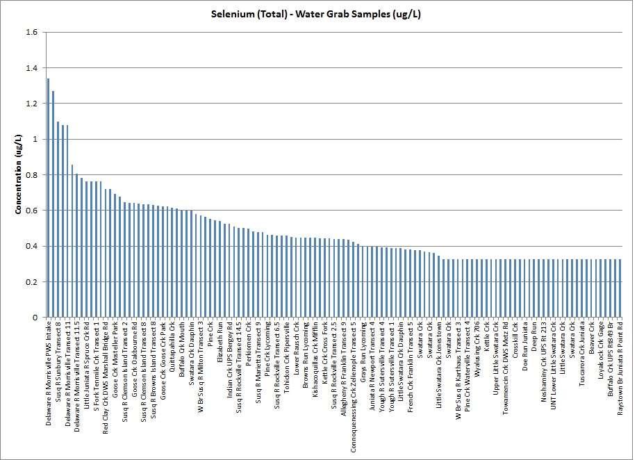
324 323

325 324

326 325

327 326

328 327

329 Candidate Cause 13: EDCs Worksheets: 43, 47, 48, and

330 Title: Hormones Analyzed from Passive Water Samplers (WS #43) Agency: Pennsylvania Department of Environmental Protection Spatial Co-occurrence using Data from the Case Candidate Cause: Toxic chemicals either kill YOY directly, or increase YOY susceptibility to disease; EDCs increase YOY susceptibility to disease Introduction: Toxic chemicals and/or EDCs could negatively affect YOY survival and/or susceptibility to disease. Water concentrations of these compounds could come into direct contact with YOY fish. If this is the case, higher concentrations of these chemicals would be expected at areas where YOY die-offs are seen and lower concentrations where no problems are seen. Data: PA DEP collected passive water samples from 12 sample sites within and out of the Susquehanna basin in 2013 to be tested for 19 hormones. Samples were analyzed at USGS: Waterbody Susquehanna River Susquehanna River Susquehanna River Susquehanna River Susquehanna River Juniata River Juniata River Susquehanna River Susquehanna River Connequenessing Creek Allegheny River Delaware River Location Name Marietta West Marietta-Falmouth East Rockville West Rockville Middle Rockville East Lewistown Narrows Newport South Sunbury West Sunbury East Zelienople Franklin Morrisville East Hormones bisphenol A diethylstilbestrol cis-androsterone epitestosterone 329

331 17-alpha-estradiol dihydrotestosterone 4-androstene-3,17- dione estrone 17-beta-estradiol testosterone equilin 11-ketotestosterone norethindrone mestranol equilenin 17-alphaethynylestradiol estriol progesterone 3-beta-Coprostanol Analysis and Results: Eight out of nineteen hormones were detected: cis-androsterone; epitestosterone; 17-alpha=estradiol; 4-androstene-3,17-dione; estrone; 17-betaestradiol; testosterone; and equilenin. 4-androstene-3,17-dione and estrone were found at every site and 17-betaestradiol was found at nearly every site (except three). Other hormones were found sporadically at different places. Allegheny R and Connoquenessing Crk had the least amount of hormones detected (only 4-androstene-3,17-dione and estrone). Juniata Newport and Lewistown, and Susquehanna Harrisburg West had the highest number of different hormones detected. There definitely seems to be a pattern of the Juniata sites and Harrisburg West site having the highest variety and concentrations of various hormones. A principal component analysis (PCA) of the hormones at each site indicate that Harrisburg West is actually quite different from the two Juniata sites. The Juniata sites, as well as Susquehanna Sunbury East, are more similar. The remaining sites (shown in the table on the previous page), including the controls, are clustered together. 330

332 331

333 332

334 Concentration (ng/l) 2013 Passive Sampler Results - Hormones (ng/l) Frank zel MVE SunW SunE Nport Ltown HRW HRE HRM MarE MarW Sites cis-androsterone epitestosterone 17-alpha-estradiol 4-androstene-3,17-dione estrone 17-beta-estradiol testosterone equilenin 333

335 Concentration (ng/l) 2013 Passive Sampler Results - Hormones (ng/l) Frank zel MVE SunW SunE Nport Ltown HRW HRE HRM MarE MarW Sites cis-androsterone epitestosterone 17-alpha-estradiol 4-androstene-3,17-dione estrone 17-beta-estradiol testosterone equilenin 334

336 Title: Hormones in Sediments (2013) (WS # 47) Agency: Pennsylvania Department of Environmental Protection Spatial Co-occurrence using Data from the Case Candidate Cause: Toxic chemicals either kill YOY directly, or increase YOY susceptibility to disease; EDCs increase YOY susceptibility to disease Introduction: Toxic chemicals and/or EDCs could negatively affect YOY survival and/or susceptibility to disease. Sediment could directly affect YOY because the eggs are laid directly on it and the young are in close contact with it. If this is the case, higher concentrations of these chemicals would be expected at areas where YOY die-offs are seen and lower concentrations where no problems are seen. Data: PA DEP collected sediment samples from 13 sample sites within and out of the Susquehanna basin in 2013 to be tested for 20 hormones. Samples were analyzed by USGS: Waterbody Susquehanna River Susquehanna River Susquehanna River Susquehanna River Susquehanna River Juniata River Juniata River Susquehanna River Susquehanna River Youghiogheny River Connequenessing Creek Allegheny River Delaware River 11-Ketotestosterone 16-Epiestriol-2,4-d2 (surrogate) 17-alpha-Estradiol Location Name Marietta West Marietta-Falmouth East Rockville West Rockville Middle Rockville East Lewistown Narrows Newport South Sunbury West Sunbury East West Newton- Sutersville Zelienople Franklin Morrisville East Equilenin Equilin Estriol 335

337 17-alpha-Ethynylestradiol 17-alpha-Ethynylestradiol-2,4,16,16-d4 (surrogate) 17-beta-Estradiol 17-beta-Estradiol-13,14,15,16,17,18-13C6 (surrogate) 3-beta-Coprostanol 4-Androstene-3,17-dione Bisphenol A Bisphenol-A-d16 (surrogate) Cholesterol Cholesterol-d7 (surrogate) cis-androsterone cis-androsterone-2,2,3,4,4-d5 (surrogate) Dihydrotestosterone Epitestosterone Estriol-2,4,16,17-d4 (surrogate) Estrone Estrone-13,14,15,16,17,18-13C6 (surrogate) Medroxyprogesterone-d3 (surrogate) Mestranol Mestranol-2,4,16,16-d4 (surrogate) Nandrolone-16,16,17-d3 (surrogate) Norethindrone Progesterone Progesterone-2,3,4-13C3 (surrogate) Testosterone trans-diethyl-1,1,1',1'-d4-stilbesterol- 3,3',5,5'-d4 (surrogate) trans-diethylstilbestrol Analysis and Results: Eleven out of twenty hormones were detected. The most commonly found were bisphenol-a (BPA), 3-beta-coprostanol, and estrone.: 17-beta-estradiol: female sex hormone; more potent in estrogenic activity than estrone/estriol (ranged ug/kg); most were estimated: (Juniata Newport (E0.25); Juniata Lewistown (0.25); Marietta East (E0.28); Susq Hbg East (E0.23); Hbg Middle (E0.50) BPA: used in production of polycarbonate plastics (ranged ug/kg; Yough = 193 ug/kg) Cholesterol: component of cell membranes, required to establish proper membrane permeability & fluidity (very imprecise, but ranged ug/kg, with Hbg Middle highest) Estrone: natural estrogenic hormone secreted by ovary & adipose tissue (found at every site except Connoquenessing, ranged ug/kg) Cis-androsterone: weak androgen (Juniata Newport only 0.47 ug/kg) 17-alpha-estradiol: isomer of 17-beta-estradiol Hbg Middle only E0.22 ug/kg) 4-androstene-3, 7-dione: testosterone precurser (found at every site except Allegheny, Connoquenessing, & West; ranged ug/kg) 3-beta-coprostanol: main sterol in feces produced by reduction of cholesterol by intestinal bacteria; often used as biomarker of human fecal matter in environment (E at every site; ranged ug/kg; Juniata Newport = E1928 ug/kg; Juniata Newport Rep = E864) 336

338 Progesterone: steroid hormone (found at 11 of 13 sites, August only; this may be factor of lab analysis rather than seasonality) Estriol: one of three main estrogens produced by human body (Susq Sunbury West = 0.16 ug/kg; Susq Sunbury East (0.57 ug/kg) Epitestosterone: natural steroid (Allegheny Franklin = ug/kg) Few patterns are noticeable in the data. Non-parametric Wilcoxon signed rank sum tests were performed; cholesterol, estrone, and progesterone significantly differed between the May and August samples. Between compounds, 17-betaestradiol & 17-alpha-estradiol, estrone & 17-alpha-estradiol, and estrone & 4- androstene-3,17-dione show significant correlations. 337

339 Concentration(ug/kg) May & August 2013 Sediment Cholesterol & 3-beta-coprostanol beta-coprostanol (May) 3-beta-coprostanol (Aug) cholesterol (May) cholesterol (Aug) Sites 338

340 Concentration (ug/kg) 3 May 2013 Sediment Hormones (no BPA) beta-estradiol estrone cis-androsterone 17-alpha-estradiol 4-androstene-3,17-dione Site 339

341 Concentration (ug/kg) 6 August 2013 Sediment Hormones Sites 17-beta-estradiol estrone cis-androsterone progesterone 17-alpha-estradiol 4-androstene-3,17-dione epitestosterone estriol 340

342 Conclusion: Few consistent patterns are noticeable in the data, but hormones remain a parameter of concern. 341

343 Title: EDCs and Intersex in Adult SMB (WS #48) Agency: Pennsylvania Department of Environmental Protection Spatial Co-occurrence using Data from the Case Candidate Cause: EDCs increase YOY susceptibility to disease and cause intersex among adult small mouth bass resulting in lower fecundity Introduction: High chronic exposure to estrogenic chemicals may increase the frequency of intersex among adult male SMB potentially resulting in lower fecundity. If this is the case, adult male SMB would have a higher proportion and severity of intersex at locations with higher concentrations of EDCs. In addition, EDCs could negatively affect YOY survival and/or susceptibility to disease. Water concentrations of these compounds could come into direct contact with YOY fish. If this is the case, higher concentrations of these chemicals would be expected at areas where YOY die-offs are seen and lower concentrations where no problems are seen. The content of this worksheet summarizes a portion of the study conducted by Vicki Blazer et. al. from USGS (Blazer et al 2014). Data: USGS collected smallmouth bass and white sucker at 16 locations in the basin and outside of the basin from 2007 to 2010 to evaluate the fish for biomarkers of estrogenic exposure including plasma vitellogenin and prevalence and severity of testicular oocyte formation in male fish. In addition, USGS collected grab discrete samples to test for 5 hormones, sediment samples to test for 7 hormones and plant sterols and, in 2010, passive samples to test for a suite of hormones and pesticides. Sites were selected in the Delaware, Susquehanna, and Ohio drainages and also were selected to bracket WWTP discharges on Brodhead Creek, Susquehanna River at Danville, and Swatara Creek. Upstream and downstream sites were selected on the Allegheny River and Monongahela River but were not focused on specific WWTP s. The locations and dates of the sampling are summarized in the table below (Table 1, reproduced from Blazer et al. 2014). 342

344 Table 1. reproduced from Blazer et al. 2014, p.6474 Analysis and Results: The percentage of male SMB with testicular oocytes was higher at the basin sites than the percentage with testicular oocytes at the out-of-basin sites (Figure 2, from Blazer et al. 2014) The percent intersex at the Schuylkill River site was intermediate and higher than the percent intersex at the Ohio basin sites but lower than the percent intersex at all of the Susquehanna River sites. The Intersex Severity Index for small mouth bass was significantly higher at the basin sites with the exception of the Swatara up and Swatara mid versus the out of basin sites (Table 4, reproduced from Blazer et al 2014). In addition, the Intersex Severity Index for SMB was significantly higher at the Juniata River site at Newport than the Allegheny River at Kittaning when considering the Spring 2010 samples, though the intersex prevalence was high in small mouth bass collected at both sites in 2010 (Juniata 67% and Allegheny 75%). Of the 5 hormones analyzed in the discrete samples, estrone and cis-androsterone were the only hormones that were detected above the reporting limit (Table 8, 343

345 reproduced from Blazer et al. 2014). Estrone and cis-androsterone were not detected in grab samples collected from the Ohio Basin. Estrone was highest in the grab samples collected from the Schuylkill River at Fall Bridge, but concentrations also exceeded reporting limits at samples collected from Brodhead Creek (downstream), Conodoguinet Creek near Hogestown, Susquehanna River (downstream of Danville WWTP), and Juniata River at Newport. Cis-androsterone was only detected in the grab sample collected from Yellow Breeches Creek at New Cumberland. Estrone concentrations were significantly correlated with testicular oocyte prevalence (rho=.6530, p=0.0238), severity (rho=0.7609, p=0.0055), and the percentage of male SMB with measurable plasma vitellogenin (rho=0.7914, p=0.0033). Estrone was the most commonly found hormone in the bed sediment with concentrations above the reporting limit at all basin sites except for the Swatara upstream site and Conodoguinet site (Table 9). Estrone was also found in the sediment at comparable levels in the out-of-basin sites including Schuylkill, Ohio, Allegheny (up and down), Monongahela (up and down), and Ohio. Estrone tended to be higher downstream of WWTPs on the Susquehanna River (Danville WWTP), and Swatara Creek. Estrone was also higher downstream of the Quittapahilla confluence. The only hormone that was found in the basin but not in the controls was progesterone, which was found at the Swatara mid and down locations, though concentrations were below the reporting limit. The androgen cis-androstene was only detected at the Ohio location. In 2010, all estrogenic and androgenic compounds tested for by the passive samplers were higher at the Juniata River site at Newport than the Allegheny River site at Kittaning (Table 10). Four out of the six pesticides tested by the passive samplers in 2010 tended to be higher at the Allegheny site including atrazine, acetochlor, metolachlor, and simazine. Prometon and desethylatrazine were below the reporting limits or detection limits at both sites. 344

346 Table 4. reproduced from Blazer et al. 2014, p

347 Figure 2. reproduced from Blazer et al. 2014, p

348 Table 8. reproduced from Blazer et al. 2014, p Table 9. Hormones and plant sterols (μg/kg) measured in sediment samples collected at fish health sites Site 17-β estradiol 17-α Estradiol Estro ne Progester one cis- Androsten e β- Sitoster ol β- Stigmastan ol MDL a Schuylkill BD BD BD Brodhead up BD BD BD BD BD 445 BD Brodhead down BD BD BD BD BD Conodoguinet BD BD BD BD 3, Susquehanna up BD BD BD BD 1, Susquehanna down BD BD BD BD 2, Swatara up BD BD BD BD BD 1, Swatara mid BD BD 6,625 1,424 Swatara down BD Juniata BD BD BD 593 BD Yellow Breeches BD BD BD BD Ohio 0.49 BD BD BD 347

349 Monongahela up BD BD BD 4, Monongahela down BD BD 2, Allegheny up BD BD BD BD 196 BD Allegheny down BD BD BD BD 177 BD a The reporting level (RL) is set at least two times higher than the method detection limit (MDL). Values at or above the RL are presented in bold; those in italics are below the RL but above the MDL and are estimated, except for β-sitosterol and β-stigmastanolwhich are all estimated due to variable method performance (Foreman et al. 2012). Below detection (BD) denotes below the MDL. Table 9. reproduced from Blazer et al. 2014, p Table 10. reproduced from Blazer, et al., 2014, p

350 Conclusion: The research conducted by Blazer et al. (2014) gives support to the hypothesis that the prevalence of testicular oocytes and severity of intersex in male smallmouth bass may play a role in the decline of YOY SMB in the lower Susquehanna basin because these reproductive benchmarks were significantly higher at the majority of the basin sites, though mean vitellogenin was similar between the Schuylkill site and the Susquehanna sites. In addition, correlation analysis demonstrated that higher levels of estrone in the water column may be associated with reproductive benchmarks in SMB but the evidence that estrone was detected at comparable levels in the sediment between basin and out of basin controls weakens the case that estrone concentration in the sediment is the cause for the decline in young of the year. The passive sampler results in 2010 gives further support that estrogenic and androgenic compounds, including 17-αestradiol, 17-β-estradiol, estrone, total EEQ, cis-androstene-3,17-dione, and testosterone, may play a role as these compounds were higher at the Juniata site than the Allegheny site, though passive samplers were just deployed at these two locations. The 2010 passive sampler pesticide results at the two sites somewhat weakens the case that the six pesticides tested for play a role because they were either below reporting limits (desethylatrazine, and prometon) or were higher at the site on the Allegheny River versus the site on the Juniata River (atrazine, acetochlor, metolachlor, and simazine). Literature Cited: Blazer, V., Iwanowicz, D., Walsh, H., Sperry, A., Iwanowicz, L., & Alvarez, D Reproductive health indicators of fishes from Pennsylvania watersheds: association with chemicals of emerging concern. Environmental Monitoring and Assessment, 186(10),

351 Title: Total Estrogenicity (WS #49) Agency: Pennsylvania Department of Environmental Protection Spatial Co-occurrence using Data from the Case Candidate Cause: EDCs increase YOY susceptibility to disease Introduction: EDCs could negatively affect YOY survival and/or susceptibility to disease. If this is the case, higher concentrations of these chemicals would be expected at areas where YOY die-offs are seen and lower concentrations where no problems are seen. Data: PA DEP collected grab samples to be tested for total estrogenicity at 29 sites within the Susquehanna River basin. Samples were analyzed by USGS: Stream Name Buffalo Creek Cocolamus Creek Crosskill Creek Earlakill Creek Elizabeth Run Frankstown Branch Juniata River Honey Creek Hungry Run Jacks Creek Juniata River below Huntington STP Juniata River below Lewistown STP Kishacoquillas Creek Little Juniata River Little Kishacoquillas Creek Little Swatara Creek 1 Little Swatara Creek 2 Lost Creek Manada Creek Quittapahilla Creek Raystown Branch Juniata River 350

352 Reeds Creek Schuylkill River Spring Creek Susquehanna Danville Susquehanna Lewisburg Swatara Creek 1 Swatara Creek 2 Swatara Creek 3 Tuscarora Creek Analysis and Results: Total estrogenicity was detected at only five sites: Crosskill Creek 0.28 ng/l Elizabeth Run 0.24 ng/l Kishacoquillas Creek 0.48 ng/l Little Swatara Creek ng/l Little Swatara Creek ng/l These arevery low amounts. There is a chance that the detection limit is not low enough to detect contaminants at the other sites. Conclusion: The evidence weakens the argument for total estrogenicity as the cause of low recruitment of YOY SMB. Few consistent patterns are noticeable in the data, but hormones remain a parameter of concern. 351

353 Candidate Cause 14: Pathogens and Parasites Worksheets: 27, 29, 30, and

354 Title: YOY Smallmouth Bass and abiotic factors (WS #27) Agency: Pennsylvania Fish and Boat Commission Stressor-Response Relationships Candidate Cause: Pathogens and parasites kill YOY directly or they are more effective because YOY have become more susceptible due to candidate causes 2-13 Introduction: One of the hypotheses is that abrupt or stressful physicochemical water quality changes at certain timeframes increases susceptibility of YOY SMB to disease. There is a complex interplay of factors that regulate disease at the individual and population levels. The presence of a pathogen is necessary but typically not sufficient to cause disease alone (Snieszko 1974). Chaplin et al. (2010) and Chaplin and Crawford (2012) documented stressful water quality conditions in nearshore, microhabitats during critical times during their development. Seifert et al. (1974) found dissolved oxygen concentrations below 4.4 mg/l resulted in a 20% reduction in survival of SMB embryos and larvae in laboratory experiments. In addition to acute effects, sub-lethal effects such as earlier hatch time and reduced growth of larval Smallmouth Bass were documented at dissolved oxygen concentrations of 4.4 mg/l (Seifert et al. 1974) while behavioral responses such as agitation and rising to the surface were documented in larval Smallmouth Bass at dissolved oxygen concentrations up to 4 mg/l (Spoor 1984). Comparisons of the Susquehanna River with similar locations at the Delaware and Allegheny rivers during found median daily maximum temperatures to be 2.0 o C, 2.7 o C, and 1.6 o C higher and 3.1 o C, 1.2 o C, and 3.4 o C higher, respectively (Chaplin et al. 2009; Chaplin and Crawford 2012). Further, a comparison of median daily temperatures from continuous monitoring data at the Susquehanna River at Harrisburg, Pennsylvania for the period critical to YOY SMB development were significantly higher (two-sided Wilcoxon signed-rank test, p < 0.05) during than during the same period in 1974 to 1979, the only other timeframe with a continuous temperature record (Chaplin et al. 2009; Chaplin and Crawford 2012). Water temperatures that YOY SMB were exposed to did not approach lethal temperatures of 37 o C suggested by Wrenn (1980) and higher temperatures during this life stage are beneficial for rapid growth, with peak consumption rates at 29 o C (Shuter and Post 1990; Hewett and Johnson 1992; Zwiefel et al.1999). Additionally, juvenile black bass (Micropterus spp.) are considered to have a higher thermal tolerance than adults (Recsetar et al. 2012). Brewer (2011) found that in spring-fed Missouri streams, age-0 353

355 SMB selected warmer available habitats regardless of the amount of groundwater contribution. At finer spatial scales, temperature is one of the primary factors with age-0 SMB habitat selections (Brewer 2011). While habitat selection based on higher temperature may benefit YOY SMB metabolically, it also potentially increases the risk of exposure to pathogens. Grant et al. (2003) found that temperatures above 30 o C increased the viral replication rate of LMBV and that Largemouth Bass infected with LMBV had higher rates of mortality and higher viral loads at 30 o C than at 25 o C in laboratory experiments. Similarly, some common bacterial pathogens such as Flavobacterium columnare (20 25 o C, Starliper and Schill 2010) and Aeromonas hydrophila (25-35 o C, Cipriano and Austin 2011) share optimal temperature ranges to that of YOY SMB. The intent of this analysis is to compare water quality conditions immediately prior to the YOY SMB surveys to determine if any factors consistently occur that may be contributing to the outbreaks. These would include elevated temperatures, elevated or variable ph, or low dissolved oxygen conditions. Data: Back-pack electrofishing CPUE (fish/ 50 m) data for YOY SMB from the Pennsylvania Fish and Boat Commission s (PFBC) state-wide monitoring network was included in the analysis. Site-specific catch and prevalence data were aggregated by river reach and by year. Timing is based on directed surveys that are tied to fish size to allow for comparable catchability among years. Surveys are point-in-time surveys and reflect conditions at the time of capture and cannot be used to infer about other conditions outside of the survey window (i.e., before or after the survey). It is assumed that environmental conditions prior to the identified survey cumulatively affect fish within the sample. Follow-up surveys noted are qualitative as fish catchability changes as they grow; results are not comparable to directed surveys but can be used to comment on presence or absence of fish with signs of disease. For Juniata River figures, lower and upper values correspond to YOY Smallmouth Bass survey results from the lower Juniata River and upper Juniata River, respectively. Physicochemical water quality data is from U.S. Geological Survey (USGS) and/or PA DEP sondes from different locations in the subject reaches. Where possible, multiple data points per location were plotted to allow for spatial differences in values to be accounted for by reviewers. The data period used was truncated to May 1 to August 14 of each year to simplify graphics while accounting for conditions that were most influential to YOY SMB. The data period for 2012 was extended to August 23 to account for the later onset of disease during that year. Analysis and Results: Continuous, instream monitoring data from subject reaches were overlain with results from PFBC directed YOY SMB surveys for subject reaches. When possible, qualitative surveys results were also overlain on the physicochemical water quality data to allow for 354

356 further analysis of factors that could have contributed to difference in disease occurrence. There is evidence of stressful water quality conditions occurring prior to the onset of disease at some reaches during some years but not occurring consistently. Further, there are also incidences where stressful water quality conditions occur where no disease is noted. There are also instances when physicochemical conditions would not be deemed particularly stressful during the time period leading into surveys; however, diseased fish were found. Throughout the different reaches and years of surveys there is no obvious pattern of physicochemical water quality conditions occurring that may be prompting disease manifestation. Conclusion: There is no evidence to support or refute the role of physicochemical parameters in the onset of disease. There are no consistent patterns in physicochemical data that precede disease onset among reaches and years. Other unmeasured factors may be present that influence the impact of these parameters. Literature Cited: Brewer, S.K Groundwater influences on the distribution and abundance of riverine Smallmouth Bass, Micropterus dolomieu, in pasture landscapes of the Midwestern USA. River Research and Applications. 29: Chaplin, J.C., J.K. Crawford, & R.A. Brightbill Water-quality monitoring in response to young-of-the-year Smallmouth Bass (Micropterus dolomieu) mortality in the Susquehanna River and major tributaries, Pennsylvania: U.S. Geological Survey Open-File Report U.S. Geological Survey, Reston, Virginia. Chaplin, J.C., & J.K. Crawford Streamflow and water-quality monitoring in response to young-of-year Smallmouth Bass (Micropterus dolomieu) mortality in the Susquehanna River and major tributaries, with comparison to the Delaware and Allegheny rivers, Pennsylvania, U.S. Geological Survey Open-File Report U.S. Geological Survey, Reston, Virginia. Cipriano, R.C. & B. Austin Furunculosis and other aeromonad diseases. Pages in P.T.K. Woo and D.W. Bruno, editors. Fish Diseases and Disorders, Volume 3: Viral, Bacterial, and Fungal Infections, 2 nd Edition. CAB International, New York.Seifert et al. (1974) Grant, E.C., D.P. Philipp, K.R.Inendino, & T.L. Goldberg Effects of temperature on the susceptibility of Largemouth Bass to Largemouth Bass Virus. Journal of Aquatic Animal Health. 15(3): Hewett, S.W. & B.L. Johnson Fish bioenergetics model 2. Technical Report WIS- SG-250, University of Wisconsin Sea Grant Institute, Madison, Wisconsin 355

357 Recsetar, M.S., M.P. Zeigler, D.L. Ward, S.A. Bonar, & C.A. Caldwell Relationship between fish size and upper thermal tolerance. Transactions of the American Fisheries Society 141: Shuter, B.J. & J.R. Post Climate, population variability, and the zoogeography of temperate fishes. Transactions of the American Fisheries Society. 119:1-34. Snieszko, S. F The effects of environmental stress on outbreaks of infectious diseases of fishes. Journal of Fish Biology 6(2): Spoor, W.A Oxygen requirements of larvae of the Smallmouth Bass, Micropterus dolomieui Lacépède. Journal of Fish Biology 25: Starliper, C.E. & W.B. Schill Flavobacterial diseases: columnaris disease, coldwater disease and bacterial gill disease. Pages in P.T.K. Woo and D.W. Bruno, editors. Fish Diseases and Disorders, Volume 3: Viral, Bacterial, and Fungal Infections, 2 nd Edition. CAB International, New York. Wrenn, W.B Effects of elevated temperature on growth and survival of smallmouth bass. Transactions of the American Fisheries Society 109: Zweifel, R.D., R.S. Hayward, & C.F. Rabeni Bioenergetics insight into black bass distribution shifts in Ozark boarder region streams. North American Journal of Fisheries Management. 19:

358 357

359 Comparison of temperature (top), ph (middle), and dissolved oxygen concentration (bottom) between main channel (gray) and microhabitat (black) locations at the Susquehanna River at Clemsons Island location during spring-summer Shaded area indicates survey window during that year with catch values for that survey reach superimposed on the graphic. 358

360 Comparison of temperature (top), ph (middle), and dissolved oxygen concentration (bottom) between main channel (gray) and microhabitat (black) locations at the Susquehanna River at Clemsons Island location during spring-summer Shaded area indicates survey window during that year with catch values for that survey reach superimposed on the graphic. 359

361 Temperature (top), ph (middle), and dissolved oxygen concentration (bottom) at the Susquehanna River at Harrisburg West channel (black line) and middle channel (gray line) locations during spring-summer Shaded areas indicate survey windows 360

362 during that year with catch values for that survey reach superimposed on the graphic. Catch values for follow-up surveys could not be reported accurately because catch biased to favor diseased fish. 361

363 Temperature (top), ph (middle), and dissolved oxygen concentration (bottom) at the Susquehanna River at Harrisburg West channel (black line) and middle channel (gray line) locations during spring-summer Shaded area indicates survey window during that year with catch values for that survey reach superimposed on the graphic. 362

364 Comparison of temperature (top), ph (middle), and dissolved oxygen concentration (bottom) between main channel (gray), microhabitat (black), and alternate (dashed gray) locations at the Juniata River at Howe Twsp Park location during spring-summer Blue line indicates survey window during that year with catch values for that survey reach superimposed on the graphic. 363

365 364

366 Comparison of temperature (top), ph (middle), and dissolved oxygen concentration (bottom) between microhabitat (black) and alternate (dashed gray) locations at the Juniata River at Howe Twsp Park location during spring-summer Blue line indicates survey window during that year with catch values for that survey reach superimposed on the graphic. 365

367 Temperature (top), ph (middle), and dissolved oxygen concentration (bottom) at the Juniata River at Newport (USGS ) location during spring-summer Blue line indicates survey window during that year with catch values for that survey reach superimposed on the graphic. 366

368 Temperature (top), ph (middle), and dissolved oxygen concentration (bottom) at the Juniata River at Newport (USGS ; gray line) and Newport North channel (black line) locations during spring-summer Blue line indicates survey window during that year with catch values for that survey reach superimposed on the graphic. 367

369 368

370 Temperature (top), ph (middle), and dissolved oxygen concentration (bottom) at the Juniata River at Newport (USGS ; gray line) and Newport North channel (black line) locations during spring-summer Blue line indicates survey window during that year with catch values for that survey reach superimposed on the graphic. 369

371 Title: Impacts of Pathogens (LMBV) or Parasites on Small Mouth Bass Populations (WS #29) Agency: Pennsylvania Fish and Boat Commission Stressor-Response Relationship Candidate Cause: New pathogens (LMBV) or parasites or intermediate hosts may have moved into the area (14b 2 ) Introduction: Factors including water quality (Chaplin et al. 2009; Chaplin and Crawford 2012; Blazer et al. 2014) and parasite pathogens (Walsh et al. 2012; Smith et al. 2014) have been associated with secondary bacterial infections that are characteristic of outbreaks among YOY SMB. Largemouth Bass Virus (LMBV) has been consistently isolated from moribund SMB specimens submitted for viral analysis. Clinically diseased fish and apparently healthy from the same location have yielded positive results for LMBV during past surveys. Despite testing positive for LMBV via cell culture, fish did not exhibit the typical clinical sign of LMBV infection described by Plumb et al. (1996). Grizzle et al. (2003), demonstrated that fish without clinical signs of disease constitute a major source of LMBV dissemination. The repeated detection of LMBV in juvenile SMB specimens from diseased populations and the coincident onset of disease and discovery of LMBV in the Susquehanna River Basin in 2005 (U.S. Fish and Wildlife Service, National Wild Fish Health Database) necessitates a closer investigation into the potential role of LMBV in causing these annual mortality episodes in juvenile SMB. Studies investigating LMBV have primarily focused on adult fish as they relate to largescale fish kills in trophy-size adult Largemouth Bass Micropterus salmoides; however, mortality has been induced in laboratory studies involving juvenile Largemouth Bass and suggest susceptibility is higher at young age and that such mortalities can be unnoticed in the field (Plumb and Zilberg 1999b, Grant et al. 2003, Inendino et al. 2005). In clinical studies, dead and moribund juvenile Largemouth Bass infected by intraperitoneal (IP) injections of LMBV had virus concentrations that averaged TCID50/g (range ), and TCID 50/g (range ) (Plumb and Zilberg 1999b). Titer loads in a small sample of moribund YOY SMB collected from the Susquehanna River Basin have been found between and (C. Hillard, Penn State University, unpublished data), which is considered high in non-experimentally infected fish. Despite species differences, similarities would suggest that there would be a similar LD 50 for LMBV in both species. Certainly, the observed viral loads in the moribund Susquehanna River SMB are similar to those observed to those associated with morbidity and mortality in Largemouth Bass in clinical trials, suggesting that LMBV 370

372 could factor in the observed mortality in the Susquehanna Basin. Unfortunately, the pathogenicity of LMBV to SMB has not been ascertained and it median lethal dose (LD 50 ) never calculated. Pathology of infected SMB has not been consistent with that documented in previous studies in the Largemouth Bass (Plumb et al. 1996, Plumb and Zilberg 1999b, Zilberg et al. 2000), suggesting differences in pathogenicity between the two closely related fish species along with the potential effects of stressors that may be prevalent at the time of infection (Groocock et al. 2008). For example, Inendino et al. (2005) found that density of fish and water quality influenced the survival and condition of juvenile Largemouth Bass infected with LMBV. Similarly, stressful water quality conditions (Chaplin et al. 2009, Chaplin and Crawford 2012, Smith et al. 2015) and the presence of opportunistic bacteria (Chaplin et al. 2009, Chaplin and Crawford 2012, Starliper et al. 2013, Smith et al. 2015) and parasite pathogens (Walsh et al. 2012, Smith et al. 2014, Smith et al. 2015) suggest that co-occurrence of these conditions in the Susquehanna River Basin may collectively exacerbate the virulence of LMBV to juvenile SMB. One key factor of interest is water temperature. YOY Smallmouth Bass condition is generally positively related to water temperature. Higher temperatures during this life stage are beneficial for rapid growth, with peak consumption rates at 29 o C (Shuter and Post 1990; Hewett and Johnson 1992; Zwiefel et al.1999). Additionally, juvenile black bass are considered to have a higher thermal tolerance than adults (Recsetar et al. 2012). However, Grant et al. (2003) found that temperatures above 30 o C increased the viral replication rate of LMBV and that Largemouth Bass infected with LMBV had higher rates of mortality and higher viral loads at 30 o C than at 25 o C in laboratory experiments. Similar to viral replication rates, many opportunistic bacteria share temperature optima with YOY SMB and may compound or utilize stress from other pathogens such as LMBV. Similarly, some common bacterial pathogens such as Flavobacterium columnare (20 25 o C, Starliper and Schill 2010) and Aeromonas hydrophila (25-35 o C, Cipriano and Austin 2011) share optimal temperature ranges to that of YOY SMB. It is plausible that despite the benefit of high water temperature to YOY SMB condition, the increased temperature could increase viral replication rate and expose fish to greater concentrations of opportunistic bacteria and could potentially induce stress and subsequently, disease. Data: Observational data for clinical signs of disease of SMB was conducted by Pennsylvania Fish and Boat Commission (PFBC) Division of Fisheries Management and Division of Fish Production Services, Fish Health Unit. Viral analysis was conducted by U.S. Fish and Wildlife Service, Northeast Fishery Center as part of the National Wild Fish Health Survey. Additional data on titer levels for some populations of SMB was provided by Penn State University, Animal Health Diagnostic Laboratory. 371

373 Results: LMBV has widespread distribution within Pennsylvania (Figure 1) since at least Generally, LMBV has been isolated from YOY SMB and Largemouth Bass from populations where fish with clinical signs of disease have been found (Table 1). This includes both apparently healthy individuals and those with clinical signs of disease, with a few exceptions. Repeated collections over the years at some locations have demonstrated that once established in a system, LMBV is not always present at detectable concentrations (Table 1, Figure 1). The role that LMBV is having in secondary infections is unknown. On-going laboratory investigations should help to clarify potential of LMBV pathogenicity to YOY SMB. Conclusion: The role of LMBV remains unclear and needs further resolution. Evidence of bass with high concentration of LMBV as well as high consistency of detection among population where disease is occurring suggest some role; however, whether it is opportunistic or primary pathogen remains unclear. It is most likely an opportunistic pathogen but it may contribute additional stress to the fish. 372

374 Table 1. Waterbody, location, date, species, sample size, disease characterization of Largemouth Bass Virus (LMBV) samples submitted as part of on-going investigations of YOY Smallmouth Bass disease investigations. Cell culture analysis and PCR confirmation was conducted by U.S. Fish and Wildlife Service, Northeast Fishery Center. Titer values were estimated by Penn State University, Animal Health Diagnotics Laboratory. Waterbody Site Date Species Number Clinical Disease LMBV Titer Comment Pine Creek 8/10/2010 Smallmouth Bass 17 Yes Yes NA Susquehanna River Danville 7/13/2010 Smallmouth Bass 21 Yes Yes NA Pequea Creek 7/28/2011 Smallmouth Bass 1 Yes No NA Pequea Creek 7/28/2011 Largemouth Bass 3 No No NA Susquehanna River Wrightsville 7/28/2011 Smallmouth Bass 12 Yes Yes NA Susquehanna River Wrightsville 7/28/2011 Largemouth Bass 1 No Yes NA Loyalsock Creek 7/27/2011 Smallmouth Bass Yes Yes NA Penns Creek 7/26/2011 Smallmouth Bass Yes Yes NA Pine Creek 7/20/2011 Smallmouth Bass 15 Yes Yes NA fish condition was very bad at time of capture Raystown Lake 8/18/2011 Largemouth Bass 15 No Yes NA No signs of clinical disease listed in table; however, picture from the field show fish with lesions Schuylkill River Cross Keys 8/3/2011 Smallmouth Bass 4 Yes Yes NA Schuylkill River Cross Keys 8/3/2011 Largemouth Bass 5 Yes Yes NA 1 fish with lesions Schuylkill River Five Locks 8/3/2011 Smallmouth Bass 10 Yes Yes NA Schuylkill River Five Locks 8/3/2011 Largemouth Bass 5 No Yes NA Delaware River Point Pleasant 8/3/2011 Smallmouth Bass 4 Yes Yes NA Delaware River Point Pleasant 8/3/2011 Largemouth Bass 4 No Yes NA Susquehanna River 7/2/2012 Smallmouth Bass No No NA Delaware River Milford 7/16/2012 Smallmouth Bass No No NA Delaware River Milford 7/16/2012 Largemouth Bass No No NA Delaware River Matamoras 7/16/2012 Smallmouth Bass No No NA Delaware River Delaware Water Gap 7/16/2012 Smallmouth Bass No No NA Lehigh River Catasauqua 7/17/2012 Smallmouth Bass No No NA Schuylkill River Port Clinton 7/18/2012 Smallmouth Bass No Yes NA Ohio River Montgomery 7/17/2012 Smallmouth Bass Yes Yes 1 x 10 4 cell culture negative for fish without signs of disease Monongahela River 7/18/2012 Smallmouth Bass No No NA Monongahela River 7/18/2012 Spotted Bass No No NA 373

375 Table 1. (cont.) Waterbody, location, date, species, sample size, disease characterization of Largemouth Bass Virus (LMBV) samples submitted as part of on-going investigations of YOY Smallmouth Bass disease investigations. Cell culture analysis and PCR confirmation was conducted by U.S. Fish and Wildlife Service, Northeast Fishery Center. Titer values were estimated by Penn State University, Animal Health Diagnotics Laboratory. Waterbody Site Date Species Number Clinical Disease LMBV Titer Comment Susquehanna River Danville 7/19/2012 Smallmouth Bass 3 No No NA Susquehanna River Danville 7/19/2012 Largemouth Bass 1 No No NA Juniata River 7/19/2012 Smallmouth Bass Yes No 1 x higher titer value in clinically / 1 x 10 diseased fish Shermans Creek 7/23/2012 Smallmouth Bass Yes Yes NA both clinically diseased and apparently healthy fish Susquehanna River Rockville 7/23/2012 Smallmouth Bass Yes Yes NA both clinically diseased and apparently health fish Bald Eagle Creek 7/24/2012 Smallmouth Bass No No NA Allegheny River 7/25/2012 Smallmouth Bass Yes Yes NA Juniata River Mifflin 7/17/2013 Smallmouth Bass 1 Yes Yes NA Susquehanna River Rockville 7/18/2013 Smallmouth Bass 3 Yes Yes NA Susquehanna River Rockville 7/18/2013 Smallmouth Bass 1 No No NA Susquehanna River Rockville 7/18/2013 Smallmouth Bass 1 No No NA Pine Creek 7/18/2014 Smallmouth Bass 20 Yes Yes NA 374

376 Figure 1: Distribution of samples analyzed for the presence of Largemouth Bass Virus (LMBV) within Pennsylvania. Data from U.S. Fish and Wildlife Service, National Wild Fish Health Database ( ). 375

377 Literature Cited: Blazer, V.S., D.D. Iwanowicz, H.L. Walsh, A.J. Sperry, L.R. Iwanowicz, D.A. Alvarez, R.A. Brightbill, G. Smith, W.T. Foreman & R. Manning Reproductive health indicators of fishes from Pennsylvania watersheds: Association with chemicals of emerging concern. Environmental Monitoring and Assessment. Chaplin, J.C., J.K. Crawford, & R.A. Brightbill Water-quality monitoring in response to young-of-the-year Smallmouth Bass (Micropterus dolomieu) mortality in the Susquehanna River and major tributaries, Pennsylvania: U.S. Geological Survey Open-File Report U.S. Geological Survey, Reston, Virginia. Chaplin, J.C., & J.K. Crawford Streamflow and water-quality monitoring in response to young-of-year Smallmouth Bass (Micropterus dolomieu) mortality in the Susquehanna River and major tributaries, with comparison to the Delaware and Allegheny rivers, Pennsylvania, U.S. Geological Survey Open-File Report U.S. Geological Survey, Reston, Virginia. Cipriano, R.C. & B. Austin Furunculosis and other aeromonad diseases. Pages in P.T.K. Woo and D.W. Bruno, editors. Fish Diseases and Disorders, Volume 3: Viral, Bacterial, and Fungal Infections, 2 nd Edition. CAB International, New York. Grant, E.C., D.P. Philipp, K.R.Inendino, & T.L. Goldberg Effects of temperature on the susceptibility of Largemouth Bass to Largemouth Bass Virus. Journal of Aquatic Animal Health. 15: Grizzle, J.M., I. Altinok, & A.D. Noyes PCR method for detection of Largemouth Bass Virus. Diseases of Aquatic Organisms 50: Groocock, G.H., S.G. Grimmet, R.G. Getchell, G.A. Wooster, & P.R. Bowser A survey to determine the presence and distribution of Largemouth Bass Virus in wild freshwater bass in New York State. Journal of Aquatic Animal Health. 20(3): Hewett, S.W. & B.L. Johnson Fish bioenergetics model 2. Technical Report WIS-SG-250, University of Wisconsin Sea Grant Institute, Madison, Wisconsin. Inendino, K.R., E.C. Grant, D.P. Philipp, & T.L. Goldberg Effects of factors related to water quality and population density on the sensitivity of juvenile 376

378 Largemouth Bass to mortality induced by viral infection. Journal of Aquatic Animal Health. 17: Plumb, J.A., J.M. Grizzle, H.E. Young, A.D. Noyes, & S. Lamprecht An iridovirus isolated from wild Largemouth Bass. Journal of Aquatic Animal Health 8: Plumb, J.A. & D. Zilberg. 1999a. Survival of largemouth iridovirus in frozen fish. Journal of Aquatic Animal Health. 11: Plumb, J.A. & D. Zilberg. 1999b. The lethal dose of Largemouth Bass Virus in juvenile Largemouth Bass and the comparative susceptibility of Striped Bass. Journal of Aquatic Animal Health. 11: Recsetar, M.S., M.P. Zeigler, D.L. Ward, S.A. Bonar, & C.A. Caldwell Relationship between fish size and upper thermal tolerance. Transactions of the American Fisheries Society 141: Shuter, B.J. & J.R. Post Climate, population variability, and the zoogeography of temperate fishes. Transactions of the American Fisheries Society 119:1-34. Smith, G.D., V.S. Blazer, H.L. Walsh, M.V. Kepler, B.P. Mangan, & C. Yamashita The role of the fish parasite Myxobolus inornatus in young-of-year Smallmouth Bass Micropterus dolomieu mortality in Pennsylvania. Final Report for PA SeaGrantSubaward 4742-COP-NOAA Smith, G.D., V.S. Blazer, H.L. Walsh, L.R. Iwanowicz, C. Starliper, & A.J. Sperry The effects of disease-related mortality of young-of-year Smallmouth Bass on population characteristics in the Susquehanna River Basin, Pennsylvania and potential implications to conservation of black bass diversity. Pages xxx-xxx in M.D. Tringali, J.M. Long, T.W. Birdsong, and M.S. Allen. Black bass diversity: multidisciplinary science for conservation. American Fisheries Society, Symposium 82, Bethesda, Maryland. Starliper, C., V. Blazer, L. Iwanowicz, & H.Walsh Microbial isolates in diseased fishes, primarily Smallmouth Bass (Micropterusdolomieu), with the Chesapeake Bay drainage in Proceedings of the West Virginia Academy of Science 85(2). Starliper, C.E. & W.B. Schill Flavobacterial diseases: columnaris disease, coldwater disease and bacterial gill disease. Pages in P.T.K. 377

379 Woo and D.W. Bruno, editors. Fish Diseases and Disorders, Volume 3: Viral, Bacterial, and Fungal Infections, 2 nd Edition. CAB International, New York. Walsh, H.L., V.S. Blazer, L.R. Iwanowicz, & G.Smith A rediscription of Myxobolus inornatus from young-of-the-year Smallmouth Bass (Micropterus dolomieu). Journal of Parasitology 98: Zilberg, D., J.M. Grizzle, & J.A. Plumb Preliminary description of lesions in juvenile Largemouth Bass injected with Largemouth Bass Virus. Diseases of Aquatic Organisms. 39: Zweifel, R.D., R.S. Hayward, & C.F. Rabeni Bioenergetics insight into black bass distribution shifts in Ozark boarder region streams. North American Journal of Fisheries Management 19:

380 Title: Impacts of Pathogens and Parasites on YOY Smallmouth Bass (WS#30) Agency: Pennsylvania Fish and Boat Commission Stressor-Response Relationship Candidate Cause: New pathogens or parasites (Myxobolus spp.) or intermediate hosts may have moved into the area. Introduction: One candidate cause that is currently being investigated is the presence of the myxozoan parasite Myxobolus inornatus (Walsh et al. 2012) within muscle and connective tissue of young-of-year (YOY) SMB Micropterus dolomieu. Myxozoan parasite infections can be responsible for important economic losses in fisheries and aquaculture industries (Sitjà-Bobadilla 2008). Myxobolus cerebralis, the parasite responsible for whirling disease in salmonids, has caused negative economic impact on recreational trout fisheries in Colorado (Nehring and Walker 1996) and other states where tourism was an important part of local and state economies (Mahoney and Hudson undated; Koel et al. 2006). Proliferate gill disease (PGD), caused by the myxozoan parasite Aurantiactinomyxon ictaluri, is the third most common disease diagnosis among commercially farmed Channel Catfish Ictalurus punctatus (Hanson et al. 2008). More recently, Sphaerospora motemarini-related mortality in juvenile Grey Snapper Lutjnaus griseus was predicted to have impacts in commercial and recreational fisheries for that species in the Gulf of Mexico (Holzer et al. 2013). Internal and external signs of parasite infections, both trematodes and myxozoans, are commonly observed in the diseased YOY SMB. The role that the myxozoan parasites play in the YOY SMB mortalities remains unclear. Parasites may compromise YOY in a number of ways: high parasite loads may contribute to general stress, as well as immune suppression, resulting in increased susceptibility to opportunistic bacteria; sites of parasite entry or exit may cause wounds allowing for bacterial entry; or heavy parasite loads may increase sensitivity to water quality related stressors. M. inornatus was first reported from Largemouth Bass fingerlings in a Montana hatchery in 1937 (Fish 1939). To our knowledge, the only other reports since then were from adult SMB 379

381 in Lake Erie with identification based on spore morphology (Dechitar and Nepszy 1988; Muzzall and Whelan 2011). Since then, the isolate from YOY SMB has been redescribed, genetically sequenced, and primer sets were developed (Walsh et al. 2012). Data: Histological data for fish collected during 2013 and 2014 from U.S. Geological Survey, Leetown Science Center, National Fish Health Research Laboratory that was funded by Pennsylvania Sea Grant. Disease incidence, prevalence, and distributional data is from Pennsylvania Fish and Boat Commission directed young-of-year black bass surveys. Analysis and Results: Very few YOY SMB were collected in 2013 with clinical signs of disease. M. inornatus (or a similar-appearing myxozoan) was observed in fish at sites in the Susquehanna drainage and one fish from the Allegheny River. Of these, only fish from the Susquehanna River at Harrisburg had clinical disease. Myxozoan cysts were not observed at sites in the Delaware drainage (Smith et al. 2014). At sites within the Susquehanna drainage fewer myxozoan parasite cysts and associated inflammation were observed in 2013 than were observed at sites with previously available data. This may be a result of changes in sample acquisition (i.e., random sample of fish rather than biased toward fish with clinical signs of disease) or lower disease incidence and prevalence during Detailed results for 2014 are pending; however, collections from 2014 documented presence of M. inornatus from fish at the West Branch Susquehanna River and Susquehanna River (Mahantango Access) where no fish were caught during A single fish with a single myxozoan cyst was found at the Lehigh River during 2014 (Table 1). Further analyses are necessary to determine if time of collection, annual differences water temperature, stream flow, or other water quality factors may influence the prevalence and severity of the infection (V. Blazer, U.S. Geological Survey, unpublished data). Based on sampling in 2013 and previous years, M. inornatus appears to be widespread in the Susquehanna River basin (Figure 1) and present at a lower incidence and severity in bass from the Allegheny and Lehigh rivers. Clinical disease was only observed at one mainstem site in the Susquehanna Basin in 2013 and at the two sites surveyed during 2014; hence evaluating the potential role of the parasite in the disease syndrome of YOY was not possible. Despite 380

382 the lack of visible lesions, there were signs of disease microscopically at the other sites including the presence of myxozoan cysts and inflammation in the muscle and connective tissue associated with myxozoan infections. It is uncertain if fish with myxozoan infections that did not have clinical disease would have developed clinical disease had they not been captured (Smith et al. 2014). An in situ hybridization technique (Antonio et al. 1998) utilizing the specific sequences identified in the species description (Walsh et al. 2012) was successfully developed by Heather Walsh, USGS National Fish Health Research Laboratory. The method identifies mature spores and immature stages within the cysts observed on young-of-year SMB. Routine handling of tissues for histopathology which includes fixation in neutral buffered formalin, sometimes for prolonged periods (weeks to months) prior to processing and decalcification of tissues in acid-based solutions were found to interfere with successful results. In 2013, some fish were fixed with the PaxGene system in order to develop the technique. While this is good for select samples, it is too expensive and timeconsuming for routine monitoring. Hence, in 2014 we experimented with routine fixation but decalcification with an EDTA solution. This appeared to be successful and the plan it to utilize this methodology in all further collections in order to 1) determine if areas of inflammation that appear to be early lesions of the SMB contain parasite DNA rather than bacterial or other factors and 2) determine if the myxozoans observed in various tissues and in SMB from various watershed are all the same species. Labeled sequences for Flavobacterium columnare together with the labeled sequences for M. inornatus will be utilized to better understand the role of each of these in the young-of-year disease progression (V. Blazer, unpublished data). Conclusion: The role of myxozoan parasites remains unclear and need further resolution. Evidence of bass with high prevalence of parasitic cysts as well as high consistency of detection among populations where disease is occurring suggest some role; however, whether it is opportunity or primary pathogen remains unclear. Regardless of its status, it may contribute additional stress to the fish. Literature Cited: Antonio, D.B., K.B. Andree, T.S. McDowell, & R.P. Hedrick Detection of Myxobolus cerebralis in rainbow trout and oligochaete tissues by using a 381

383 nonradioactive in situ hybrization (ISH) protocol. Journal of Aquatic Animal Health. 10: Dechitar, A.O. & S.J. Nepszy Survey of the parasitic fauna of selected fish species from Lake Erie, Pages In S.J. Nepszy, ed. Parasites of fishes in the Canadian waters of the Great Lakes. Great Lakes Fishery Commission Technical Report No. 51. Ann Arbor, Michigan. Fish, F.F Notes on Myxobolus inornatus n. sp., a myxosporidian, parasitic in the black bass (Huro floridana, Le Sueur). Transactions of the American Fisheries Society 68: Hanson, T.R., S. Shaik, K.H. Coble, S. Edwards, & J.C. Miller Identifying risk factors affecting weather- and disease-related losses in the U.S. Farm-Raised Catfish Industry. Agricultural and Resource Economics Review 37(1): Holzer, A.S., H. Pecková, S. Patra, N.P. Brennan, C. Yanes-Roca, & K.L. Main Severe glomerular disease in juvenile grey snapper Lutjanus griseus L. in the Gulf of Mexico caused by the myxozoan Sphaerospora motemarini n. sp.. International Journal for Parasitology: Parasites and Wildlife 2(2013): Koel, T.M., D.L. Mahony, K.L. Kinnan, C. Rasmussen, C.J. Hudson, S. Murcia, & B.L. Kerans Myxobolus cerebralis in Native Cutthroat Trout of the Yellowstone Lake Ecosystem. Journal of Aquatic Animal Health 18: Nehring, R.B, & P.G. Walker Whirling disease in the wild: the new reality in the Intermountain West. Fisheries 21(6): Mahony, D. & C. Hudson. Undated. Distribution of Myxobolus cerebralis in Yellowstone Cutthroat Trout Oncorhynchus clarki bouvieri in Yellowstone Lake and Tributaries. Project Completion Report. Muzzall, P.M. & G. Whelan Parasites of fish from the Great Lakes: a synopsis and review of the literature, Great Lakes Fisheries Commission Miscellaneous Publication Ann Arbor, Michigan. Sitjà-Bobadilla, A Fish immune response to Myxozoan parasites. Parasite 15: Smith, G.D., V.S. Blazer, H.L. Walsh, M.V. Kepler, B.P. Mangan, & C.Yamashita The role of the fish parasite Myxobolus inornatus in young-of-year 382

384 Smallmouth Bass Micropterus dolomieu mortality in Pennsylvania. Final Report for Pennsylvania SeaGrant Subaward No COP-NOAA Walsh, H.L., V.S. Blazer, L.R. Iwanowicz, & G.Smith A rediscription of Myxobolus inornatus from young-of-the-year Smallmouth Bass (Micropterus dolomieu). Journal of Parasitology 98: Table 1. The catch, number and percentage of fish with clinical signs of disease, and the presence of myxozoan cysts in young-of-year SMB at various locations within Pennsylvania during 2013 and Clinical signs of disease are visual assessments in the field while myxozoan determination is by histological analysis by U.S. Geological Survey, Leetown Science Center, National Fish Health Laboratory. Waterbody Location Drainage Catch Disease d # (%) Presence of Myxozoa n Delaware River Matamoras Delaware 0 NF 1 No Lehigh River Northampton Delaware 15 0 No Lehigh River Northampton 2 Delaware 21 0 Yes 3 Schuylkill River Port Clinton Delaware 25 0 No Elk Creek Lake Erie 21 0 No Allegheny River Buckaloons Ohio 32 0 Yes 3 Allegheny River Buckaloons 2 Ohio 9 0 No Juniata River Susquehann a River Susquehann a River Susquehann a River Susquehann a River Susquehann a River West Branch Susquehann a River Thompsontow n Susquehanna 5 0 Yes Danville Susquehanna 9 0 No Harrisburg Susquehanna 28 4 (14.3) Yes Laceyville Susquehanna 23 0 Yes Mahantango Susquehanna 0 NF NF Mahantango 2 Susquehanna 18 9 (50.0) Yes Watsontown Susquehanna 0 NF NF 383

385 West Branch Susquehann Watsontown 2 Susquehanna a River 11 5 (45.4) Yes 1 - no fish in initial survey; however, follow-up survey yielded enough fish for analysis 2 - site revisited during 2014 to capture adequate sample 3 - record indicates a single cyst found in a single fish Figure 1. Distribution of Myxobolus inornatus in tissues of young-of-year (YOY) SMB Micropterus dolomieu during 2013 and Circles indicate locations where no fish (NF) were captured during initial surveys. Triangles indicate locations where YOY SMB were found but did not display clinical symptoms (No) of disease and did not have myxozoan cysts present during histological analysis. Squares indicate locations where YOY SMB had myxozoan cysts present (Yes) during histological analysis but either had no clinical signs of disease (hollow) or had clinical signs of disease (black filled). Initial surveys at the Delaware River at Matamoras yielded no YOY SMB; however, a follow-up collection produced 384

386 enough fish for histological analysis. Additional collections were made at four locations during 2014 where either no fish were found or where additional fish were needed for analysis. 385

387 Title: Disease Prevalence in YOY Smallmouth Bass (WS #31) Agency: Pennsylvania Fish and Boat Commission Stressor-response associations from the case Candidate Cause: Disease Introduction: If diseases were causing the lack of recruitment into the adult SMB population, we would expect a negative correlation between the prevalence of disease and year 1 catch per unit effort (CPUE). Data: Source: Pennsylvania Fish and Boat Commission Disease prevalence Disease prevalence is the proportion of YOY SMB captured during backpack electrofishing surveys at each site displaying clinical signs of disease compared to the overall catch at that give site. Prevalence is reported at reach-wide aggregates in this instance (total catch with signs of disease in the reach/ total catch within the reach * 100). Prevalence values are index values reported during initial, directed surveys to maintain consistency among years. Directed surveys focus on a period of time when fish are 45 mm 75mm TL to maintain similarities in catchability. Catchability of fish outside of that size range decreases and may affect results; primarily, biasing catch towards compromised fish (i.e., sick fish easier to catch, inflating prevalence values) Age-1 CPUE Age-1 catch per unit effort (CPUE; fish/h) was calculated reach-wide from boat electrofishing surveys for adult SMB at large river reaches state-wide. Age indices were used to calculate the component of catch across each reach that was attributable to Age-1 fish within a given year. Cumulative, reach-wide effort (electrofishing time (in hours) was then applied to the reach-wide catch data to determine CPUE. Analysis and Results The association between disease prevalence and the next year s Age-1 CPUE was calculated using Spearman s rank correlation. Spearman s rank correlation (r) = A scatterplot of the relationship is shown in Figure

388 Figure 1. A scatterplot of disease prevalence of young of the year smallmouth bass (YOY) vs. Age 1 smallmouth bass catch per unit effort in the following year. Conclusion: Disease was strongly and negatively associated with Age-CPUE. This supports the hypothesis that disease is playing a role in recruitment of SMB to adult age classes. 387

389 Worksheets not used as Evidence in the CADDIS Decision Process Worksheets: 41, 43, and

390 Title: Chemical Compounds in the Susquehanna River Basin (WS # 41) Agency: Pennsylvania Department of Environmental Protection Spatial Co-occurrence using Data from the Case Candidate Cause: Toxic chemicals either kill YOY directly, or increase YOY susceptibility to disease; EDCs increase YOY susceptibility to disease Introduction: Toxic chemicals and/or EDCs could negatively affect YOY survival and/or susceptibility to disease. Water concentrations of these compounds could come into direct contact with YOY fish. If this is the case, higher concentrations of these chemicals would be expected at areas where YOY die-offs are seen and lower concentrations where no problems are seen. Data: PA DEP collected passive water samples from 12 sample sites within and out of the Susquehanna basin in 2013 to be tested for a variety of different compounds (organochlorine & currently used pesticides, PCBs, PBDEs, hormones, wastewater indicators, and PAHs pharmaceutical data is currently pending): Waterbody Susquehanna River Susquehanna River Susquehanna River Susquehanna River Susquehanna River Juniata River Juniata River Susquehanna River Susquehanna River Connequenessing Creek Allegheny River Delaware River Location Name Marietta West Marietta-Falmouth East Rockville West Rockville Middle Rockville East Lewistown Narrows Newport South Sunbury West Sunbury East Zelienople Franklin Morrisville East 389

391 Analysis and Results: Juniata Lewistown and Newport are clustered together towards the end of axis 2; Susquehanna Marietta East and West are also clustered together. The remaining Susquehanna sites are clustered together and the control sites are scattered and somewhat separated from the Susquehanna basin sites. Juniata sites are definitely similar, and tend to have a large number of compounds (as can be seen below), while the Susquehanna sites are more similar to each other. The controls, however, also tend to have high numbers of compounds and are not true reference sites. 390

392 391

393 # of Compounds Passive Samplers - Total # of Compounds per Site (not including pharmaceuticals) Frank Zel MVE SunW SunE HRW Sites HRE HRMid MarE MarW NPort Ltown TOTAL # OF COMPOUNDS 392

394 Title: Stroud Study Temperature Cycling and Maximum Temperature Effects on SMB (WS #54) Agency: Pennsylvania Department of Environmental Protection Candidate Cause: High Water Temperatures (and changing water temperatures) Introduction: DEP contracted Stroud Water Research Center to perform a study on the effect of rate of temperature change (abruptly changing temperatures) and various thermal maxima on fish and macroinvertebrates. The fish that were studied were walleye, white sucker, golden shiner and smallmouth bass; however, this worksheet will focus on smallmouth bass. The smallmouth bass were generally more tolerant than the other fish species to both temperature maxima and rate of temperature change. Study Design: The study included 2 experiments and was conducted in 2010 and It should be noted that Stroud conducted a rate of temperature change study for PPL in which the results were reported in The PPL study was designed to evaluate sub-lethal effects of temperature changes on biological organisms and therefore included lower temperatures (82 F or cooler) than what see typically see in the Susquehanna in midsummer in order to avoid mortality. DEP then decided to take the PPL study further and look at higher temperatures which we often see as ambient temperatures in big rivers and also frequently where thermal discharges occur. In DEP Experiment 1, four fish species were exposed to two constant (82 or 89 F) or one of three fluctuating temperature regimes (2, 4, or 8 F/h) for 30 days under midsummer (75-89 F, mean 82 F) conditions. The total degree hours were equalized among regimes by adjusting the time spent at the maximum and minimum temperatures. Fish were acclimated to 82 F over three weeks prior to initiating the experiment. Sub-lethal response was assessed by measuring the primary, secondary, and tertiary stress response (cortisol, glucose, or triglyceride, respectively) during the first day of temperature fluctuation and again after 4 weeks of temperature cycling; by periodically measuring growth and survival; and by histopathology analysis of a number of tissues at the conclusion of temperature cycling. DEP Experiment 2 was aimed at determining the effect of the upper temperature reached during diel fluctuations on the stress response. Fluctuations went from 75 F to a maximum temperature of 82 F (August ambient), 87 F, 89 F, 91 F, or 93 F, where the rate of change was 4 F/hour and time at maximum temperature was 10 hours 393

395 across treatments. All fish were acclimated to 75 F over two weeks prior to initiating the experiment. The same sub-lethal stress responses were monitored as for Experiment 1. Results: Experiment 1: SMB did not show a primary stress SMB exhibited significantly lower growth in the 89 F treatment (control) Some SMB showed some interesting characters but appeared to be unrelated to temperature cycling: curved spines; focal branchitis and lamellar fusion of the gills; intersex gonads; flukes without an associated inflammation reaction in the river and spleen Antagonistic behavior among SMB during acclimation period led to low initial survival of SMB but there was 100% survival once they were isolated other than a few that died shortly after being moved due to injuries sustained earlier 394

396 Experiment 2: Cycling to 91 F stressed or killed SMB Temperature cycling appeared to drive the increase in cortisol at the peak temperatures but returned to baseline levels during the ramp down and at the lower soak temperature (decreasing temperatures offered relief) Cortisol levels in SMB in the 91 F and 93 F treatments were significantly elevated at the peak temperature after 30 days of temperature cycling. They were also elevated in the 91 F treatment at the bottom of the diel cycle 395

397 Metabolism did not appear to be affected by treatments (glucose and triglycerides) 5 SMB developed curved spines in experiment thought to be unrelated to temperature 2 SMB found to be moribund during quarantine showed severe infestations of gills, kidney necrosis hemorage, flukes in the gastrointestinal tract and liver, suggested that fish arrived from Schuylkill river in a heavily infested state Almost all SMB showed signs of lesions, inflammation or parasite infestation and some had extreme liver vacuolation. Tissue damage or parasite infestation appeared to increase sensitivity of other species (walleye and golden shiner) to extreme temperature changes but did not appear to alter the sensitivity of the SMB (or white sucker) Withdrawing blood from SMB for bioassays created more stress than expected Among SMB not sampled for blood, there was significant mortality among fish reaching 93 F All [normal spine] SMB that died, did so within 48 hours of reaching the peak temperature for the first time 396

398 397