Baltic Marine Environment Protection Commission

Transcription

1 Baltic Marine Environment Protection Commission Expert Working Group for Mutual Exchange and Deliveries of AIS & Data Stockholm, Sweden, 7-8 June 2017 AIS EWG Document title Draft methodology to create statistics and density maps from AIS data Code 6-2 Category DEC Agenda Item 6 - Access to and use of HELCOM AIS information Submission date Submitted by Secretariat Reference Outcome of AIS EWG , Paragraphs Background HELCOM Automated Identification Systems (AIS) data is currently used for several purposes in the Baltic Sea, for example improving navigation safety, analyzing emissions from ships or mapping underwater noise. The HELCOM Secretariat has not been able to make use of this data due to lack of resources and many projects in the HELCOM community have not taken advantage of this valuable information. Due to funding opportunities, the HELCOM Secretariat has been recently able to use AIS data to provide shipping density maps as well as statistics. Learning how to handle the large AIS dataset has not been an easy task: the tools were created from scratch to produce AIS data products. The part 1 of the document will explain the methodology used by the HELCOM Secretariat to prepare the AIS data to for producing maps and statistics. The part 2 will explain how to generate shipping density maps. Action requested The Meeting is invited to consider the attached guidelines to create statistics and density maps from AIS data with a view of publishing as HELCOM publication and methodology annex of the maritime assessment. Page 1 of 20

2 Draft methodology to create statistics and density maps from AIS data Background 1 Action requested 1 INTRODUCTION 3 PART 1: METHODS TO PRODUCE STATISTICS 3 SHIPS MOVEMENTS: THE EXIT AND ENTER EVENTS 4 SHIP MOVEMENTS IN THE BALTIC SEA 8 OUTPUTS OF THE PROCESS 11 PART 2 METHODS TO PRODUCE DENSITY MAPS 13 WHAT IS A SHIPPING DENSITY MAP 13 WHAT WE NEED BEFORE CREATING THE DENSITY MAPS 14 What software we need to create shipping density maps: 14 Monthly csv files 14 What grid do we need? 15 THREE STEPS FOR CREATING DENSITY MAPS 15 1 Create lines 15 2 Split lines by ship type 16 3 Make the density map 17 Page 2 of 20

3 Introduction HELCOM Automated Identification Systems (AIS) data is currently used for several purposes in the Baltic Sea, for example improving navigation safety, analyzing emissions from ships or mapping underwater noise. The HELCOM Secretariat has not been able to make use of this data due to lack of resources and many projects in the HELCOM community have not taken advantage of this valuable information. Due to funding opportunities, the HELCOM Secretariat has been recently able to use AIS data to provide shipping density maps as well as statistics. Learning how to handle the large AIS dataset has not been an easy task: the tools were created from scratch to produce AIS data products. The part 1 of the document will explain the methodology used by the HELCOM Secretariat to prepare the AIS data to for producing maps and statistics. The part 2 will explain how to generate shipping density maps. Part 1: Methods to produce statistics The aim of this analysis is to produce monthly CSV files with which we can create maps and statistics based on HELCOM AIS data. To create those CSV files we worked with monthly files of pre-processed AIS data. This document explains how we add parameters to those files: Trips: Ships going from port to port. Stops: Ships stopping in a port Exits: Ships exiting the Baltic Sea Enters: Ships entering the Baltic Sea To identify these parameters, we created four types of areas. Our method tracks the ship movements between them: Exiting and entering areas of the Baltic Sea Areas outside the Baltic Sea Ports where the ships are stopping The Baltic Sea area where the ships are traveling Before this process was started, the AIS data was pre-processed to clean it and make it human readable and to remove erroneous signals. This part was done by the HELCOM Secretariat with data from the AIS HELCOM Server managed by the Danish Maritime Authority until end of Since the beginning of 2017 the server is administered by the Norwegian Coastal Administration. The following methodology was automatically repeated to each monthly files of AIS data from April 2005 to 2016 included and only for IMO-registered ships. Most of the computing tasks were done using the software R (V3.3.1) with the R Studio interface (R ). For some GIS tasks we used ArcGIS 10.4 for Desktop. The server used has the following specifications: Intel Xeon E ,30GHz 10 cores with 48 GB RAM. The method we explain outputs two files: - A CSV file with a trip Id numbers to produce density maps - A CSV file describing the ships movement. Page 3 of 20

4 Ships movements: the exit and enter events This first section will explain how to identify the ships going outside and entering the Baltic Sea, area defined by the Article 1 of the Helsinki Convention. The output of this analysis are the exit and enter events table. It is a list describing which ships are leaving or entering the Baltic Sea, at what time and where. 1. Definition of the signals The very first step is to find the AIS signals from ships that could be leaving or entering the Baltic Sea. The signals are by definition the position reports from ships. The latitude and longitude are the two parameters used for this spatial analysis. We defined 5 areas as exit areas : the borders between outside and inside the Baltic Sea where the ships have to go through to leave the Baltic Sea towards the North Sea or to major lakes in the Baltic Sea Region (Lakes Vänerm, Ladoga and Saimaa). These areas are polygons between 2,4 and 16,6 km wide. Name of the exit area Skagen Goteborg Kiel Canal Neva River Lappenrenta Location Between the port of Skagen (Denmark) and the village of Kärna located 15 km north of Gothenburg (Sweden). On the Göta Canal next to the city of Kungälv (Sweden). This location marks the entrance and exit to the Vänerm lake in central Sweden. On the Kiel Canal on the Western side of the port of Kiel (Germany). This location marks a canal between the Baltic Sea and the North Sea. Along the Neva river, after the city of Saint-Petersburg (Russia). This location is used to assess the ships going to or coming from the lake Ladoga in Russia. On the Saimaa Canal, between the Gulf of Finland the Saimaa lake. We created a new column called exit area in the table (position reports from ships). For each signals that are in one of the 5 polygons, the name of the exit area was added to this new column. We also defined a second type of polygons to highlight the areas outside the Baltic Sea: a total of 4 polygons were created and are naturally located next to each of the exit polygons previously described. They are called outside areas. Name of the outside area Skagen / Vänerm Kiel Saimaa Neva River Location The area of the North Sea (outside the Kattegat Sea towards the North Sea) and the Vänerm lake. The Kiel Canal. The Saimaa lake The Neva River and the Ladoga lake Page 4 of 20

5 We added a new column to the table to identify the signals that are outside the Baltic Sea hence inside these outside areas. The figure 1 below is showing the two exit areas Skagen and Goteborg and the outside area Skagen / Vänerm. The signals that are not in the exit area or in the outside area are obviously in the Baltic Sea. These are signals from ships in ports or traveling in the Baltic Sea therefore they are in an area called inside area. Fig. 1: Location of outside and exit areas, example of the Kattegat Sea. 2. Identification of the sequences of signals in the exit areas of the Baltic Sea After the previous step, we could know the location of each AIS signals: in an exit area of the Baltic Sea, outside the Baltic Sea or in the Baltic Sea. By sorting the data by ship (IMO number) and by time, we identified the sequences of ships traveling through the exit areas polygons. A sequence is a group of signals from a ship describing a movement the exit areas. The figure 2 (below) illustrates how we built that sequence. Each one has a unique identification number: the signals are gathered into groups of signals that match the same sequence. Page 5 of 20

6 Fig. 2: Generating the sequences in an exit area. In the figure 2, the points X 6, X 7 and X 8 have the same sequence identification number. The points from X 218 to X 220 have another unique identification number. But the points from X 105 to X 108 do not have a sequence identification number: the ship is not leaving the Baltic Sea since there is no point in the outside area. This process is applied for all of the signals found in the exit areas. We give the sequence identification number to the ships following two kind of paths: inside area -> exit area -> outside Baltic or outside Baltic -> exit area -> inside area For the ships that are returning to the same area (outside or inside) than they came from, there is no sequence identification number added to the signals. 3. Definition of the sequences entering or exiting the Baltic Sea Each of the signals of AIS data have a parameter called COG the course over ground (a value from 0 to 360 ). Following the COG of the signals within these 5 polygons, we could identify if the ships were entering or leaving the Baltic Sea. The 5 exit areas polygons were located to identify the ships leaving or entering the Baltic Sea. For each signals that have a sequence identification number, a new value defining a Page 6 of 20

7 unique direction of the boat was assigned. For example, if the boat is traveling between 90 and 270 in an exit area, we can say that the boat is traveling towards the south: the value 180 is added for this signal (for 180 ). This step is done for each signals in the exit area: a new value is added (0 for traveling north, 90 for traveling east, 180 for traveling south and 270 for traveling west). This new value is called COG 2. The next step was to identify all the sequences leaving or entering the Baltic Sea through the exit areas. A function available with the software R (under the package dplyr) was used to summarize the COG 2 for each of the unique sequences and therefore the direction of the ships within the exiting area. The average of the COG2 (x COG2) was computed for each of the unique sequences. We made these calculations of COG 2 and x COG2 to avoid some unexpected ship movements in the exit areas. Finally, we selected the signals from ships going outside or inside the Baltic Sea for each exits area following the name of the location of these unique sequences: Name of the exit area Value of x COG2 for exiting the Baltic Sea Value of x COG2 for entering the Baltic Sea Skagen x COG2 = 0 (north) x COG2 = 180 (south) Goteborg x COG2 = 180 x COG2 = 0 Kiel Canal x COG2 = 270 (west) x COG2 = 90 (east) Neva River x COG2 = 90 x COG2 = 180 Lappenrenta x COG2 = 0 x COG2 = 180 After this step, we could know if the ships was exiting or entering the Baltic Sea for each exit area and for each sequence. 4. Creation of the events exit / enter The next step was to create the exit and enter events for each of the unique sequence identification number. An event is the information about the exits and enters of the Baltic Sea: Parameters created for the exit and enter events IMO number MMSI number MinTime MaxTime Event Location Sequence number Definition IMO number of the ship MMSI number of the ship Date and time of the first signal in the exit area Date and time of the last signal in the exit area Exit or Enter the name of the exit area The unique sequence of the exit or enter After the events are identified, we could know the time of exiting or entering the Baltic Sea through the 5 exit areas for each ship. This new data was stored in a temporary file and was used during the last step of the analysis. Page 7 of 20

8 Ship movements in the Baltic Sea The second section of the analysis was to create the trips and the stops events - a table with stops in ports and trips between ports or between a port and exit/enter areas. 1. The ports of the Baltic Sea First, we created 245 ports polygons around ports in the 9 countries of the Baltic Sea. We used this method: We filtered some monthly AIS data keeping only the signals where the speed of the boat was 0. We used Open Street Map, Google Maps as background images. Shipping lines produced with AIS data helped to see ship movements The publication Baltic Ports List of 2012 helped to identify ports. 2. Definition of the signals: where are the ships? Once the ports polygons were ready we wanted to check if the ships where inside or outside those areas. We plotted in R software the AIS signals and overlaid them on top of the ports polygons and the exit areas. 3. Preparation of the signals defining a stop in a port To locate the ships that are stopped in a port we used the speed of the ship which is available as the parameter SOG (Speed Over Ground) for each position reports. In theory, just filtering those ships with SOG equals zero would be enough. However, because of the accuracy of the AIS transmitter onboard the ships, it is possible that the SOG is not equal to 0 even when the ship is at berth in a port. To avoid this issue, the SOG of a ship at port with less than 0.5 knot was replaced by 0 knot. When the speed was equal or higher than 0.5 knot, we kept the original SOG the boat could be moving during the maneuver along the berth. 4. Producing the events stops in a port The next step was to generate the events stop: a group of signals with a unique sequence identification number. Each signals that were qualified as a stop from the previous step would be assigned this number. To find the stops as sequences we sorted the data by ship (IMO number) and by time. The table would show when a ship is at sea and coming into a port and is stopping (when the SOG value is equal to 0). The sequence identification number is given to the ships following two kind of paths: at sea -> at stop or stop -> at sea Page 8 of 20

9 Finally, we created the following parameters by summarizing the information by each unique identification number: Parameters created for the Definition stops sequences IMO number IMO number of the ship MMSI number MMSI number of the ship MinTime Date and time of the first signal with SOG = 0 MaxTime Date and time of the last signal with SOG = 0 Event Stop Location the name of the port Sequence number The unique sequence of stop Once we calculated the Mintime and Maxtime, it was possible to know the duration of the stops. Thereafter, we made a subset of the stops longer than 10 minutes is done which was stored as a temporary file to be used later. 5. Producing the events trips at sea After the stops at port were created we proceeded to calculate the trip of each trip at sea. Naturally, all the signals outside the 245 port polygons and in the Baltic Sea were selected as trips. To find the trips between two stops, between an enter and a stop and between a stop and an exit, we sorted the data the data by ship (IMO number) and by time The figure 3 below shows three types of situation: the signals as trips between an exit area and a stop (situation 1), between two ports (situations 2) or between a port and an exit area (situation 3). Page 9 of 20

10 Fig. 3: The 3 types of situations for the trips sequences We assigned a unique sequence number, called the trip Id, to each movements between the locations. Every signals of the same sequence will have assigned the same sequence number, called trip Id (cf. Fig. 4 below). This is the input needed to produce lines and shipping density maps. The same process was applied to all of the ships. Page 10 of 20

11 Fig. 4: Assigning the trip ID value to the sequences at sea These are all the parameters that we calculated: Information collected for the trip sequences IMO number MMSI number MinTime MaxTime Distance sailed Event Sequence number Definition IMO number of the ship MMSI number of the ship Date and time of the first signal of the trip Date and time of the last signal of the trip Distance sailed Trip The trip Id value To calculate the duration of each trips we could use Mintime and Maxtime. The distance sailed was calculated during the summarizing step it is the cumulative distance between each signals of the trip Id value. This table is saved as temporary file and will be used for the next step. Outputs of the process The output of the whole process are two CSV files. The first one is used to produce statistics of the events: they have to be harmonized to be relevant for further analysis. The second one is the file with the position reports from ships with a trip Id assigned to each AIS signals. These monthly files are used to produce shipping density maps. Page 11 of 20

12 Output to produce statistics Output to produce density maps Three files per month: - A table with the exit / enter sequences information - A table with the stop sequences information - A table with the trip sequences information Monthly files with a trip Id assigned to each AIS position report. With which we can produce density maps. These three table are merged and sorted by ship (IMO number) and time. However, the files have to harmonize: for the same ship, two stop sequences or visit sequences cannot be consecutive. If some of them are consecutive, they are merged together and the duration of the events and the distance sailed at sea is corrected. The monthly files are finally merged as yearly files to generate statistics on a yearly basis Page 12 of 20

13 Part 2 Methods to produce density maps What is a shipping density map A shipping density map represents the intensity of shipping traffic in certain time period. There is no standard definition or method to create shipping density maps. We have developed a method that answers a basic question: Assuming we have a grid of cells and the trips of ships from port to port, how many times do those trips cross each cell of the grid? The process can be explained in four steps: 1 We need a grid with 1km*1km cells 2 We overlap the trips of each ship onto the grid 1km 1km 3 We count how many lines are crossing each cell 4 We apply the style darker color means more density Page 13 of 20

14 What we need before creating the density maps Before we begin to produce shipping density maps we need: The right software Monthly CSV files with all the AIS signals A grid to overlap the lines and create the maps A ship list: a csv file containing all ships per year. What software we need to create shipping density maps: We used ArcGIS 10.4 for Desktop advanced license with Spatial Analyst for creating raster layers. All scripts were written in python scripting language version 2.7 using ArcPy a Python ArcGIS scripting module. We used a dedicated server available through remote access with the following specifications: Intel Xeon E ,30GHz 10 cores with 48 GB RAM. Monthly csv files We have to be sure we create beforehand the following folders under each year. O1_trips is created in a previous process. It contains a CSV file per month: Each monthly file contains the following columns: Page 14 of 20

15 What grid do we need? We need a grid, a shapefile with square cells, in order to put the lines on top. We then count how many of them are crossing each cell. The grid file was downloaded from the European Environment Agency (EEA) and it is based on recommendations made at the 1st European Workshop on Reference Grids in 2003 and later from INSPIRE geographical grid systems. This standard grid was recommended to facilitate the management and analyses of spatial information for a variety of applications. EEA offers a grid in shapefile format for each country in three scales: 1km, 10km and 100km. We chose the 1km grid to produce high resolution maps. After we downloaded each Baltic Sea country we joined them all in one file. The resulting merged grid had more than four millions cells. We then delete the cells on land to save space and make the file easier to manage. The result was a file with about 400,000 cells. Three Steps for creating density maps Once we have the monthly csv files with the AIS signals, the folders and the grid we can start the process to create a density map. We followed three steps to create density maps: 1. Create lines 2. Divide the lines in ship types 3. Make the density map There is a python script for each step. They all use python s multiprocessing module. This module allows us to submit multiple processes that can run independently from each other in order to make best use of our CPU cores. We used a machine with 10 cores. The final result of processing one year is a density map in raster format (TIFF) per month and per ship type. That makes 96 maps. It takes about 40 hours to complete the process on average per year. All scripts will be made available in the HELCOM Secretariat GitHub. 1 Create lines NAME OF THE SCRIPT: TrackBuilderFromCSV_multiprocessing.py PURPOSE: Creates lines representing trips of ships from port to port. DURATION: three hours per year with multiprocessing. PRECONDITIONS: Before creating lines we need: A year folder under which there are csv files containing all trips per month. Page 15 of 20

16 The file name of the monthly file must have the year and the month name in English The monthly csv file must have the following columns: o MMSI o Trip_id: Number of trips per MMSI (per ship) HOW THE SCRIPT WORKS: This script reads each monthly csv file and converts coordinates to lines OUTPUT: the output of this process is a folder with lines shapefiles for each month 2 Split lines by ship type NAME OF THE SCRIPT: SplitTracksByShipType_multiprocessing.py PURPOSE: Once we have the lines shapefiles we proceed to divide each file into different ship types DURATION: two hours per year with multiprocessing. PRECONDITIONS: Before creating lines we need: A folder with monthly lines shapefiles Page 16 of 20

17 The file name of the monthly file must have the year and the month in English A ship list: a csv file with unique number of ships per year created in a previous step. This file must include at least the following fields: o IMO number o HELCOM_Gr: HELCOM Gross ship type a wide classification of ship types o HELCOM_De: HELCOM Detail ship type a detail classification HOW THE SCRIPT WORKS: This script divides the monthly line files into the HELCOM gross classification ship types: "CARGO", "CONTAINER", "FISHING", "OTHER", "PASSENGER", "SER- VICE", "TANKER", "UNKNOWN", "VEHICLECARRIERROROCARGO" OUTPUT: a folder per ship type under which there are the monthly lines shapefiles 3 Make the density map NAME OF THE SCRIPT: CreateRastersYear_multiprocessing.py PURPOSE: Create a density map by overlapping a grid and counting the number of lines crossing each cell Page 17 of 20

18 DURATION: It depends on the ship type. We estimate an average of 5h per ship type. For cargo, the ship type with most signals, it takes about 10 hours. A ship type with less signals as service can take about 2h. PRECONDITIONS: Before creating lines we need: A folder with monthly lines shapefiles divided in ship types The file name of the file must have the year and the month in English A grid shapefile (go or link to page 1) HOW THE SCRIPT WORKS: The process to create a map is divided into six steps, illustrated in the figure below. It uses python s multiprocessing module to run six months simultaneously: Page 18 of 20

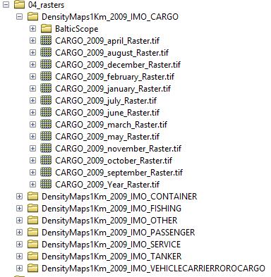
19 OUTPUT: a folder, 04_rasters, with subfolders for each ship type. Under each subfolder there is a raster file in TIFF format for each month. There is also a yearly file (CARGO_2009_Year_Raster.tif) with the sum of all monthly raster files Page 19 of 20

20 Page 20 of 20