Econ 1101 Summer 2013 Lecture 3. Section 005 6/19/2013

Transcription

1 Econ 1101 Summer 2013 Lecture 3 Section 005 6/19/2013

2 Announcements Homework 2 is due tonight at 11:45pm, CDT Recitation is tomorrow at the end of the class prepare questions about the homework or lecture contents if you have any. Another Aplia experiment (price ceilings): 2

3 Agenda for today 1. The concept of elasticity 2. Related case study 3. Income elasticity of demand 4. Other types of elasticities 5. Econland 6. Pareto Efficiency 7. Link between Pareto efficiency and market allocation (The Adam Smith Theorem) 3

4 Elasticity Last class: discussed direction of effects. For example: (1) own price then Q D (2) substitute price then Q D This class: beyond the direction, we are interested in the magnitude. Sure Q D when own price. But by how much? Sure Q D when substitute price. But by how much? 4

5 Elasticity, cont d Responsiveness of demand and supply to changes. What kinds of changes? Three types we will look at: 1) Price 2) Income 3) Price of a related good Perhaps we can just use the slope? D D D 2 1 P D D P2 P1 Nope, defective because of units issue. Cannot compare two goods this way. Example: A $1 increase in price causes a decrease in quantity demanded of 5000 beads A $1 increase in price causes a decrease in quantity demanded of 1 can of spam Q Q Q 5

6 Elasticity, cont d Get units out by using percentages e D = Price elasticity of Demand (midpoint method: gives us same elasticity between two points) % Q D P Q2 1 Q2 2 P2 1 P 2 2 Q 1 Q P 1 P 1 1 6

7 Elasticity, cont d Maybe this will help Think about a rubber band, you apply force to it to see how much it changes in its shape. Similarly, the force is now price (for price elasticity of demand), income (for income elasticity of demand), or price of a related good (for cross price elasticity of demand) and the shape is now quantity demanded. How responsive is quantity to price? Or income? Or the price of a related good? 7

8 Graphically Which one is more responsive to a change in price? 8

9 Elasticity, cont d Perfectly inelastic demand e D = 0 Examples: 9

10 Elasticity, cont d Perfectly inelastic supply e S = 0 Examples: 10

11 Elasticity, cont d Perfectly elastic demand e D = infinity Examples: 11

12 Elasticity, cont d Perfectly elastic supply e S = infinity Examples: 12

13 Elasticity, cont d In between cases: (1) When e D < 1 we say: Demand is Inelastic Total Spending = P*Q increases as P increases. (Basically, if price goes up by 1%, quantity demanded goes down by less than 1%) (2) When e D > 1 we say: Demand is Elastic Total Spending = P*Q decreases as P increases. (Basically, if price goes up by 1%, quantity demanded goes down by more than 1%) (3) When e D = 1 we say: Demand is Unit Elastic (Basically, if price goes up by 1%, quantity demanded goes down by exactly 1%) Let s try to calculate e D in an example. 13

14 Example Time Period Per Capita Daily Consumption of Motor Gasoline Average Price Per Gallon in Dollars June June Δ Average of both Years %Δ

15 Example, cont d So e D % Q D % P.28 Short-Run Demand is Inelastic As price goes up, Total Spending = P*Q increases. 15

16 Example, cont d When estimating demand elasticity, we need to hold fixed other determinants of demand in order to isolate the impact of the change in price. Why? Ex: Price elasticity of demand What are we trying to find? What happens if we don t hold other factors fixed? Also need to take into account supply. Some of you might be thinking: Why is what we calculated the elasticity of demand and not the elasticity of supply? 16

17 Example, cont d $ June 2008 S June 2007 S D Q 17

18 Example, cont d $ Q 18

19 Example, cont d We show that it is the demand elasticity by seeing that: The supply curve did shift: Price of barrel of oil increased from $65 to $121. Oil is an input in making gasoline. An increase in input prices shifts the supply curve up and to left. Demand Curve Did Not Shift (So movement along Demand) Have to argue that the determinants of demand (the things that make it shift) remained unchanged. 19

20 Example, cont d Let s go through the determinants of demand 1) Tastes of consumers Seasonality in Demand (drive more in summer than spring). Hold this fixed here by comparing June to June. 2) Number of consumers Population grows over time. Hold fixed here by using per capita numbers. 20

21 Example, cont d 3) Income Gas is a normal good. So in order for demand not to shift, income can t change. Income not that much different June 2007 to June (But things started looking different later in 2008, as the economy started falling off a cliff on account of the economic crisis.) 4) Prices of substitutes and complements Didn t change much over this one year period. 21

22 Long Run Elasticity Elasticity we have estimated is a short-run elasticity. Consumers have not had much time to make a response. Over a long period of time, if gas is significantly higher in price: Consumers will buy different cars Might live in different places Society might change the laws, like lower the speed limit. For the long-run elasticity, we need to compare cases where prices have been different for a long time. 22

23 Case Study Let s take a look at Reading 2: Fuel Consumption in Europe and the U.S. Europe has long taxed gasoline. What we pay here at the pump for gas wouldn t pay the tax in the Europe. The tax here is (per gallon): Federal 18.4 cents State (MN) 40.4 Total (MN) 58.8 (23 cents more in CA) 23

24 Case Study, cont d 24 Country Average Price $US per Gallon Consumption Per Capita Gallons Per Day United States Selected Countries in Europe Norway 7.00 * United Kingdom Germany France Spain Italy Some Other Countries Japan Mexico China Per Capita GDP ($1,000)

25 Case Study, cont d Price and Per Capita Quantity Consumed of Gasoline The United States and Norway in 2007 Time Period Per Capita Daily Consumption of Motor Gasoline Average Price Per Gallon in Dollars United States (the now ) Norway (the future ) Δ Average of Both Periods %Δ So: Elasticity(long run) = %ΔQ/%ΔP = 1.24/.86=

26 Case Study, cont d Is this valid? 1) Is Supply Curve is shifting between these two countries? Yes. Because the tax on gas in Norway shifts the supply curve up and to the left. 2) Is Demand Curve staying fixed? Have to analyze this step by step: A) Income We picked Norway because income is approximately the same as US. Note gas is a normal good so we need to be careful to hold fixed income in the comparison. Look in the table at China s consumption of gas. It is small because China is still a poor country. What about price of substitutes? (i.e. what are some substitutes?) 26

27 Case Study, cont d B) Price of Substitutes Oops. Public transit is more convenient in Norway, it is a better option. The availability of a substitute shifts the demand for gas down and to the left. So our simple analysis gives the higher price too much of the credit for the lower consumption in Norway. Demand for gas in Norway is lower both because the price of gas is higher and because public transit is better. So the actual elasticity is lower than the 1.44 estimate above. (i.e. instead of saying a 1% increase in price causes a 1.44% decrease in quantity, some of that decrease in quantity is due to availability of substitutes and not just because of the 1% price increase) 27

28 Case Study, cont d C) Other Factors Population Density? Population density is lower in the US than Europe and that is one reason demand for gas is higher in US. (But Norway is less dense than most European countries, so Norway and U.S. comparison is not as bad) 28

29 Summary What Makes Demand More Elastic? 1. Long time horizon 2. Luxury, not a necessity. 3. When products are defined more narrowly so there are better substitutes. Look at Food A) Price elasticity of food as a group is low (inelastic). So if all prices increase by 10%, quantity falls less than 10% (so spending on food goes up). Price of food goes up overall, you still need to eat. 29

30 Summary B) But now suppose look at one kind of food, meat. Raise price of meat, price of other foods fixed... Some possibilities for substitution: fish, bread, etc. C) Now look at raising price of Johnsonville Brats 10% Can easily substitute a different brand of brat, so very responsive to changes in price. 30

31 Income Elasticity of Demand e Incom e % Q D Income If Income Elasticity of Demand (IED) > 0, the good is.. If Income Elasticity of Demand (IED) < 0, the good is. 31

32 Income Elasticity of Demand For Normal Goods: Two kinds: Necessity (Or income inelastic. Spending share falls as income rises) toilet paper Luxury (Or income elastic: Sending share rises as income rises) vacation homes... and 32

33 Income Elasticity of Demand Health Care (At country level) Look at this data on health care spending as percent of GDP (gross domestic product) for various countries Data from, Uwe E. Reinhardt, Peter S. Hussey and Gerard F. Anderson, "U.S. Health Care Spending In An International Context," Health Affairs, 23, no. 3 (2004):

34 Income Elasticity of Demand GDP per Capita Health Spending Share County US Switzerland Norway Germany Canada Average Rich Hungary Slovak Rep Mexico Turkey Average Poor So health care at the country level is clearly an income elastic good. Richer countries tend to spend a higher share of income on health care. 34

35 Introducing Econland Now, let s look at something different: let s introduce a model that we will use to study how markets work. As is standard practice in economics, the model will be fully specified. We will be explicit about all the agents in the economy and how they behave. 35

36 Econland Our toy economy that follows some explicit assumptions. Like the map example from the first day of class, what happens in Econland can tell us something useful about the real world. Useful because we can use Econland to examine the efficiency of competitive markets and the impacts of government policies. Inhabitants: D1, D2, D3,.D10 and S1, S2, S3,.,S10 Only D (Demand) people eat Widgets, and each D person can eat at most one widget. Each D person has a reservation value for one widget. Amount of dollars he would be exactly willing to give up to get one. 36

37 Table of Reservation Values Name Reservation price for one widget D1 9 D2 8 D3 7 D4 6 D5 5 D6 4 D7 3 D8 2 D9 1 D10 0 Suppose D1 has $20 to start with. D1 indifferent between: $20 and 0 widget Or $11 and 1 widget (he values a widget a $9, so $20-$9 = $11) 37

38 Suppliers S people: Don t eat widgets But know how to make them However, they get hungry from widget work (so they won t do it for free!) Cost to an S person to make one widget can be interpreted as the amount of dollars we have to give her so she is just willing to do it. 38

39 Table of Costs Cost of one Name widget (dollars) 1 S1 2 S2 3 S3 4 S4 5 S5 6 S6 7 S7 8 S8 9 S9 10 S10 Suppose S3 has $20 to start with. S3 indifferent between: $20 and making 0 widget Or $23 and making 1 widget (She must get $3 from selling a widget to be still indifferent) 39

40 Putting it together 40 Name Res. Price Cost Name D1 9 1 S1 D2 8 2 S2 D3 7 3 S3 D4 6 4 S4 D5 5 5 S5 D6 4 6 S6 D7 3 7 S7 D8 2 8 S8 D9 1 9 S9 D S10

41 From the society s point of view Marginal Cost: the cost of the next one in (think of the additional cost to sellers as a group due to the next unit) Marginal Reservation Price: The value of the next one in (or additional value to buyers as a group that the next unit provides) Often referred to as marginal benefit 41

42 Plotting it on a graph 42

43 Econland Suppose we set up a market economy in Econland At P=3, who is willing to sell? So Q S is So from Marginal Cost curve, we get At P=7, who is willing to buy? So Q D is Name Res. Price Cost Name D1 9 1 S1 D2 8 2 S2 D3 7 3 S3 D4 6 4 S4 D5 5 5 S5 D6 4 6 S6 D7 3 7 S7 D8 2 8 S8 D9 1 9 S9 D S10 So from Marginal Reservation Price curve, we get 43

44 Econland What happens when Econland is a Market Economy? P: Price of a widget MRP is demand curve MC is supply curve Equilibrium: Q = 5 P = $5 S1, S2, S3, S4, S5 produce D1, D2, D3, D4, D5 consume 44

45 Gains from trade What are the gains from trade (being in the market)? Consumer Surplus (CS) of particular buyer = reservation price price paid Producer surplus (PS) of seller = price received cost 45

46 Surplus in Econland Q Res. price CS Price Cost PS Price paid rec

47 Surplus in Econland Consumer Surplus is $10 Producer Surplus is $10 Total Surplus is just Consumer Surplus + Producer Surplus So Total Surplus = $20 in this example 47

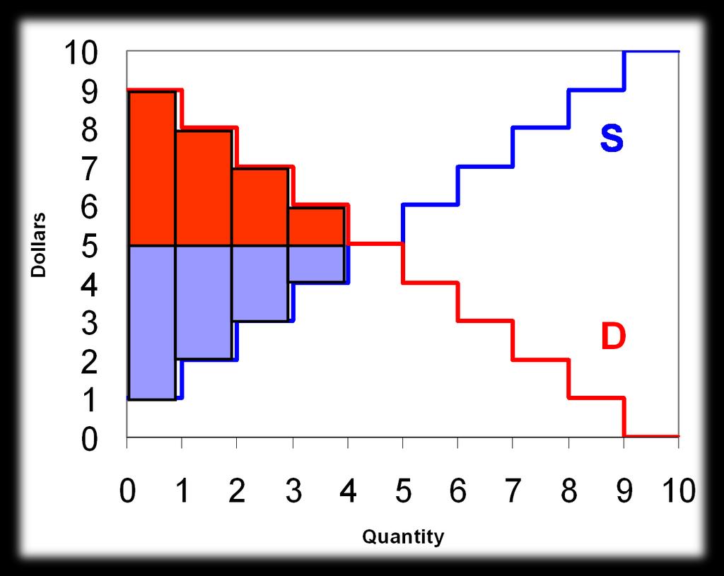
48 Graphically 48

49 Surplus in Econland Consumer Surplus Area between demand curve and price line Producer Surplus Area between price line and supply curve In Econland, demand and supply curves look like steps In economy with lots of people, we won t notice the steps, things will smooth out (this example had 10 people, but think about an economy with 1000 people, the steps will become smaller. Now think about an economy with infinitely many people) 49

50 General Case CS = Area of Triangle = ½ 5 5 = 12.5 PS = ½ 5 5 = 12.5 TS = CS + PS = 25 50

51 Efficiency We just have the same supply and demand diagram that we ve always been looking at. This is the case when the allocation is a market allocation (P, Q, and Who are determined competitively) How should we interpret this new Total Surplus idea? Look at it like a Social surplus or if it helps, a Social pie Consumers get part of the social pie, producers get part of the social pie. But can we say that the market allocation is efficient? What does it mean for an allocation to be efficient? We need a concept of efficiency. The standard concept in Economics is Pareto Efficiency 51

52 Pareto Efficiency Vilfredo Pareto An allocation is Pareto Efficient if it is feasible and there is no way to make someone better off without making someone worse off. Alternatively: The Pie is big as it can be. (If someone is to get a bigger slice, it can only come from someone else getting a smaller slice.) 52

53 Example There are 6 pieces of a cake. Are the following allocations Pareto efficient? 2 pieces to the student, 2 pieces to me, and 2 pieces in the trash 4 pieces to me, 2 pieces to the student 6 pieces to me, none for the student 8 pieces to me, none for the student Where does equity show up in the definition of efficiency? 53

54 Pareto Efficiency Name Res. Price Cost Name D1 9 1 S1 D2 8 2 S2 D3 7 3 S3 D4 6 4 S4 D5 5 5 S5 D6 4 6 S6 D7 3 7 S7 D8 2 8 S8 D9 1 9 S9 D S10 Let s go back to the Econland numbers Reservation Prices and Costs for Widgets 54

55 Pareto Efficiency 1. Suppose we have an allocation where D8 consumes a widget but D2 does not. Is this Pareto efficient? Nam e Res. Pric e Cost Name D1 9 1 S1 D2 8 2 S2 D3 7 3 S3 D4 6 4 S4 D5 5 5 S5 D6 4 6 S6 D7 3 7 S7 D8 2 8 S8 D9 1 9 S9 D S10 55

56 Pareto Efficiency 2. Suppose we have an allocation where S7 produces a widget but S1 does not. Is this Pareto efficient? Nam e Res. Pric e Cost Name D1 9 1 S1 D2 8 2 S2 D3 7 3 S3 D4 6 4 S4 D5 5 5 S5 D6 4 6 S6 D7 3 7 S7 D8 2 8 S8 D9 1 9 S9 D S10 56

57 Something to think about Then what is a Pareto Efficient allocation in Econland? 57

58 Before the break We introduced the concept of efficiency. We asked whether the market allocation (where equilibrium is determined by supply equal to demand) is an efficient one. Definition of efficiency we will use in class: Pareto efficiency An allocation is Pareto efficient if it is feasible and you cannot make someone better off without making someone worse off Remember the cheesecake example (6 slices of cheesecake total) Pareto efficient if I get 5, student get 2? Pareto efficient if I get 6, student get 0? Pareto efficient if I get 2, student gets 2? 58

59 Before the break, cont d Remember: Pareto efficiency says NOTHING about equality! I could have all the cheesecake and we will call that Pareto efficient. So, you can think of a Pareto efficient allocation as one that maximizes the social pie. Do you like the concept of Pareto efficiency? Is it too restrictive? Or maybe too weak? 59

60 A different idea Kaldor-Hicks efficiency: an outcome can still be considered efficient if those who are better off could compensate somehow those who are worse off (even if in fact no compensation will actually take place). Think of a huge public investment project (e.g. factory, highway), which is protested by a single household who enjoy living in peace and quiet. 60

61 We ended last class with two examples Name Res. Cost Name Price D1 9 1 S1 D2 8 2 S2 D3 7 3 S3 D4 6 4 S4 D5 5 5 S5 D6 4 6 S6 D7 3 7 S7 D8 2 8 S8 D9 1 9 S9 D S10 61 Suppose we have an allocation where D8 consumes a widget but D2 does not. Is this Pareto efficient? No. D2 could give D8, say, $3 and both are better off (D8 only values consuming a widget at $2, and he s getting $3 while D8 only pays $3 for a widget, where he values it at $8) Suppose we have an allocation where S7 produces a widget but S1 does not. Is this Pareto efficient? No. S7 could outsource to S1 basically not producing anything but paying S1 $2 (for example) to produce a widget. S1 benefits since that s more than cost, S7 benefits because they make a widget for only $2 instead of $7.

62 So how do we get an allocation that is Pareto efficient? What is a Pareto efficient allocation in Econland? (the question we left off with last class) Let s look at some general principles of efficient allocations. 62

63 General Principle 1 Efficient allocation of consumption: In any efficient allocation, consumers with the highest willingness to pay consume. So remember from the Econland example, D2 has higher willingness to pay than D8, but D8 consumes first, so this allocation is not efficient! 63

64 General Principle 2 In any efficient allocation, producers with the lowest cost produce. But how much to produce? How do we know how many lowest cost producers should produce? 64

65 Example Back to Econland. Name Res. Cost Name Price D1 9 1 S1 D2 8 2 S2 D3 7 3 S3 D4 6 4 S4 D5 5 5 S5 D6 4 6 S6 D7 3 7 S7 D8 2 8 S8 D9 1 9 S9 D S10 Consider an allocation where 3 widgets are produced (by S1, S2, S3) and 3 widgets are consumed (by D1, D2, and D3). Pareto efficient? 65

66 Example Back to Econland. Name Res. Cost Name Price D1 9 1 S1 D2 8 2 S2 D3 7 3 S3 D4 6 4 S4 D5 5 5 S5 D6 4 6 S6 D7 3 7 S7 D8 2 8 S8 D9 1 9 S9 D S10 Consider an allocation where 8 widgets are produced (by S1-S8) and 8 widgets are consumed (by D1-D8). Pareto efficient? No. Relative to the initial allocation, S8 can give $5 instead of a widget. Paying $5 is cheaper for S8 than making a widget. D8 would rather have $5 than a widget. So both better off, no one worse off. 66

67 Lesson What did we learn from these two examples? When Q=3, there is someone out there (D4) not consuming who is willing to pay more than it will cost someone (S4) to produce. So raise quantity. When Q=8, there is someone out there consuming (D8) who is willing to pay less than what it is costing someone (S8) to produce. So lower quantity. From this, we get 67

68 General Principle 3 Efficient Quantity In any efficient allocation, the quantity is where the marginal valuation of the last unit consumed equals the marginal cost of the last unit produced. Principles 1, 2, and 3 imply that in an efficient allocation for the widget industry in Econland: Q = 5 S1, S2, S3, S4, S5 produce D1, D2, D3, D4, D5 consume 68

69 Graphically Q efficient = 5, Social Surplus equals: = All of this should look familiar. Let s link this to the market.

70 Big Idea Q = 5, S1, S2, S3, S4, S5 produce, D1, D2, D3, D4, D5 consume Market Allocation is Pareto Efficient! 70

71 First Welfare Theorem Assume: 1. Market structure is perfectly competitive (not monopoly or oligopoly) 2. No externalities (my action hurts or benefits others, but I don t take into account - like pollution.) Then the unregulated market (laissez-faire) allocation is Pareto efficient. (It maximizes the size of the social pie.) 71

72 First Welfare Theorem, cont d Also called Adam Smith Theorem Remember quote about invisible hand? Every individual... neither intends to promote the public interest, nor knows how much he is promoting it (but) by directing that industry (to) its greatest value, he is led by an invisible hand to promote an end which was no part of his intention. 72

73 First Welfare Theorem, cont d The First Welfare Theorem also sometimes called: Adam Smith Theorem or Invisible Hand Theorem Now while the market maximizes the size of the pie (under the assumptions given above), you might not like the way it is divided up. Market delivers on efficiency. Not necessarily on equity. 73