Managers require good forecasts of future events. Business Analysts may choose from a wide range of forecasting techniques to support decision making.

Transcription

1 Managers require good forecasts of future events. Business Analysts may choose from a wide range of forecasting techniques to support decision making. Three major categories of forecasting approaches: 1. Qualitative and judgmental techniques 2. Statistical time-series models 3. Explanatory/causal models

2 Qualitative and Judgmental techniques rely on experience and intuition. They are necessary when historical data is not available or when predictions are needed far into the future. The historical analogy approach obtains a forecast through comparative analysis with prior situations. Does not always work for oil prices The Delphi method questions an anonymous panel of experts 2-3 times in order to reach a convergence of opinion on the forecasted variable.

3 Indicators are measures that are believed to influence the behavior of a variable we wish to forecast. Forecasting GDP is often done using leading indicators (series that change before the GDP changes) and lagging indicators Leading - formation of business enterprises - S&P 500 stock prices Lagging - business investment expenditures - prime rate - inventories on hand Indicators are often combined quantitatively into an index, a single measure that weights multiple indicators, thus providing a measure of overall expectation. Example: Dow Jones Industrial Average

4 A stream of historical data, such as weekly sales T = number of periods, t = 1, 2,, T Time series have 4 components: - trends (upward or downward) - seasonal effects - cyclical effects - random behavior

5 A seasonal effect is one that repeats at fixed intervals of time, typically a year, month, week, or day.

6 Cyclical effects describe ups and downs over a much longer time frame, such as several years.

7 Stationary time series have only random behavior. Moving average model Exponential smoothing model to be used over short time periods when trend, seasonal, or cyclical effects are not significant

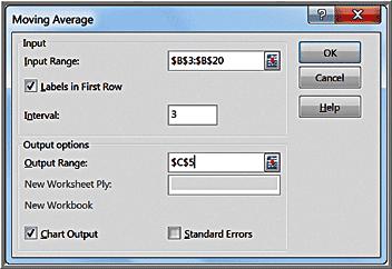
8 Computed as the average of the most recent k observations. Three-period moving average forecast for week 18

9

10 Mean absolute deviation (MAD) Mean square error (MSE) Root mean square error (RMSE) Mean absolute percentage error (MAPE)

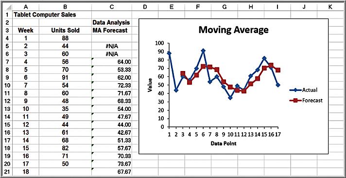
11 Tablet Computer Sales data 2-, 3-, and 4-period moving average models 2-period model has lowest error metric values

12 F t+1 is the forecast for time period t + 1, F t is the forecast for period t, A t is the observed value in period t, a is a smoothing constant (= damping factor) between 0 and 1 Forecast for week 3 when α = 0.7: (1 0.7)(88) + (0.7)(44) = 57.2

13 Note that Damping factor = 1 α The first cell of the Output Range should be adjacent to the first data point

14 Using linear trendline

15 When autocorrelation is present, successive observations are correlated with one another; for example, large observations tend to follow other large observations, and small observations also tend to follow one another. In such cases, other approaches, called autoregressive models, are more appropriate.

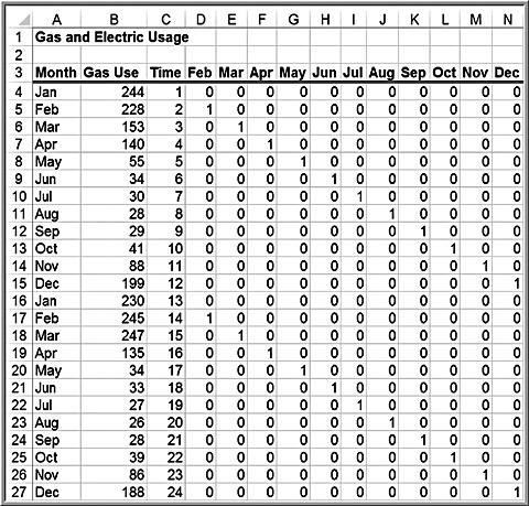
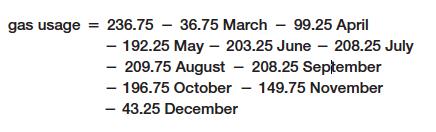
16 Use a seasonal categorical variable with k = 12 levels. Construct the regression model using k - 1 dummy variables, with January being the reference month.

17

18

19 Simple trendline using week as the independent variable Predicted sales for week 11 = (11) = 13,733 gallons

20 In many forecasting applications, other independent variables besides time, such as economic indexes or demographic factors, may influence the time series. Explanatory/causal models, often called econometric models, seek to identify factors that explain statistically the patterns observed in the variable being forecast, usually with regression analysis The average price per gallon changes each week, and this may influence consumer sales. Average price per gallon is a causal variable. Develop a multiple linear regression model to predict gasoline sales using both time and price per gallon.

21 Multiple regression model Predicted sales for week 11 = 72, (11) 16,463(3.80) = 15,368

22 Judgmental and qualitative methods are used for forecasting sales of product lines and broad company and industry forecasts. Simple time-series models are used for short- and medium-range forecasts. Regression methods are typically used for longterm forecasts.