Lecture 3: Further static oligopoly Tom Holden

Transcription

1 Lecture 3: Further static oligopoly Tom Holden

2 Game theory refresher 2 Sequential games Subgame Perfect Nash Equilibria More static oligopoly: Entry Welfare Cournot versus Bertrand Kreps and Scheinkman (1983)

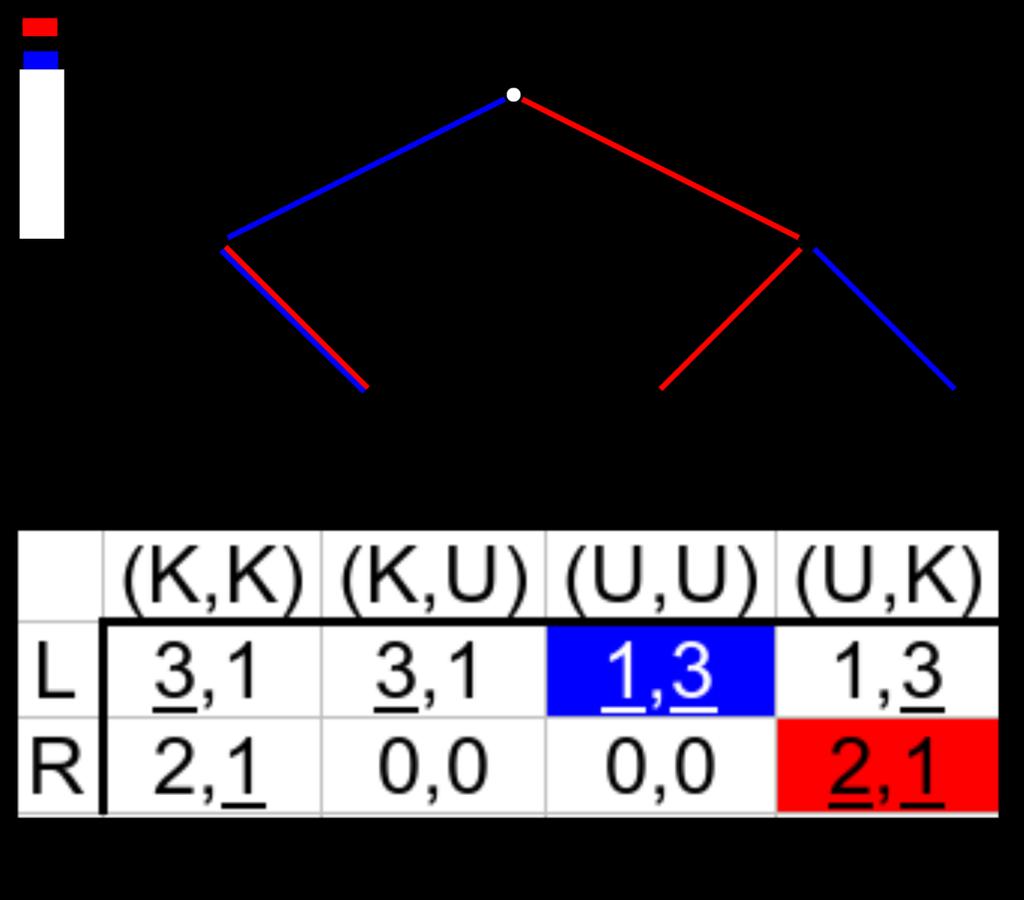
3 L R K U K U 3:1 1:3 2:1 0:0 Source: Wikimedia Commons lainingexample.svg

4 Idea: at any point in time, whatever s happened up to that point, from that point forward people will play the Nash equilibrium. And players know this in advance. A Nash equilibrium is a sub-game perfect Nash equilibrium (SPNE) if and only if at every node in the game tree, the actions it specifies at that node constitute a Nash equilibrium of the sub-game. Important: Must hold even for nodes that are never reached in equilibrium! Solve for SPNE by backwards induction. Start at the leaves (the last period) and work backwards.

5 The Centipede game: Consider two players: Alice and Bob. Alice moves first. At the start of the game, Alice has two piles of coins in front of her: one pile contains 4 coins and the other pile contains 1 coin. Each player has two moves available: either "take" the larger pile of coins and give the smaller pile to the other player or "push" both piles across the table to the other player. Each time the piles of coins pass across the table, the quantity of coins in each pile doubles. For example, assume that Alice chooses to "push" the piles on her first move, handing the piles of 1 and 4 coins over to Bob, doubling them to 2 and 8. Bob could now use his first move to either "take" the pile of 8 coins and give 2 coins to Alice, or he can "push" the two piles back across the table again to Alice, again increasing the size of the piles to 4 and 16 coins. The game continues for a fixed number of rounds or until a player decides to end the game by pocketing a pile of coins. Source: _%28game_theory%29

6 Suppose it is Alice s turn and the fixed number of pushes has expired. Then Alice has no choice but to take the big pile, which is of size 8n where 2n is the size of the smaller pile. Now think about what Bob would do the turn before. At that point, the big pile is of size 4n and the small pile is of size n. So he can either take 4n now, or wait and get 2n from Alice. Now think what Alice would do the turn before that, etc.

7 Two periods In period 1, firms simultaneously decide whether or not to enter the industry. Those that enter pay a fixed cost of F. In period 2, firms set quantities or prices, and produce. We solve period 2 first, then find optimal behaviour in period 1 given expectations of what will happen in period 2.

8 Assume that all potential entrants have the same marginal cost. And assume that monopoly profits (π M ) are bigger than the entry cost, F but less than infinity. Suppose one firm decides to pay the entry cost. In the second stage it will choose the monopoly price, and make an overall profit of π M F. Suppose more than one firm decides to pay the entry cost. In the second stage all firms will set price equal to marginal cost, and thus make an overall profit of F (i.e. a loss).

9 So only one firm will enter! We get monopoly precisely because competition would yield the competitive outcome. When potential entrants have different marginal costs, which will enter?

10 When is welfare improved by the government paying the entry cost for two firms? When the DWL due to monopoly is greater than F. Recall DWL is the area between the demand and the MC curves for quantities between the monopoly one and the competitive one. I.e. when QM Q PC p Q c dq > F where: c is marginal cost, Q M is the monopoly quantity Q PC is the perfectly competitive quantity. Exercise: simplify this condition in the special case of linear demand (p Q = p 0 p 1 Q).

11 Assume iso-elastic demand p Q = kq β and that all firms have constant marginal costs c. So under Cournot: p Q = c exercise). And Q = kn βk cn 1 β 1 β n (shown in last week s Thus, firm production profits are: p Q c Q n = c 1 β n c Q n = 1 n βc n β kn βk cn 1 β

12 If production profits were less than F, at least one firm would want to deviate to not entering. Thus profits must be greater than F. But it must also be the case that if one extra firm entered, it would make a loss overall. Thus n is the largest integer such that 1 n βc n β kn βk cn 1 β > F. For large markets, this means 1 n βc n β kn βk cn 1 β F.

13 What happens to the number of firms in an industry as the size of the market increases? 1 1 Here kβ measures the size of the market. kβ doubles, demand doubles (at any price). From the entry condition: n 1 kβ 1 F βc n β n β cn 1 β Thus, the number of firms grows more slowly that the size of the market.

14 Intuition: if price did not adjust as more firms entered, then the entry condition would always keep n k 1 β constant. But price is falling as the market gets larger, so firms are less keen to enter. Thus firms are larger in larger markets. (A general result for Cournot.)

15 Campbell and Hopenhayn (2005) Regress average firm size in an industry on number of firms and assorted controls. Find firms are larger in larger industries. Bresnahan and Reiss (1991) Call the market size required to support exactly n firms S n. We should have S n+1 > n+1 S n n (I.e. to grow by one firm, market size needs to grow by a larger amount than the number of firms.) They find this holds for small n, but for n 4, S n+1 S n Suggestive of attaining perfect competition. n+1 n.

16 Total social surplus (consumer + producer) Q is: n 0 p Q c dq nf where Qn is the total produced with n firms. We want to know if welfare would be increased by adding more firms. So we differentiate welfare with respect to n, which gives: p Q n c dq n F dn

17 But at the equilibrium number of firms (n ): F p Q n c Q n thus, the derivative of welfare w.r.t. n at n is the value of the following expression, evaluated at n = n : p Q n c dq n F F n dq n dn Q n dn 1 n2 dq n 1 = F Q n dn n Q n n 2 = F n2 d Q n Q n dn n < 0 (as quantity produced by each firm is decreasing in the number of firms). n Thus welfare would be increased by decreasing the number of firms.

18 Intuition: an entrant does not internalise the damage it does to the desired quantity produced by other firms. Business stealing effect. Ceases to hold if new entrants are producing slightly different products.

19 Bertrand: firms set prices, quantities adjust to clear the market. The software industry? Cournot: firms set quantities, prices adjust to clear the market. Without a process of price-adjustment requires a mysterious auctioneer to set prices. Large manufacturing, e.g. cars, airplanes, etc? Characterised by production quantity decisions being performed in advance.

20 Period 1: Firms invest in capacity. Period 2: Firms compete in price subject to the constraint that production is less or equal to capacity. Result: like Cournot. Kreps and Scheinkman (1983)

21 Firms i 1,2 : Each with zero marginal cost for simplicity. Firm i cannot produce more than q i (exogenous). Firms choose prices p i. Market demand Q p. Suppose firm 1 sets a price p 1 < p 2 at which Q p 1 > q 1. Then demand exceeds supply, so some rationing must occur.

22 Suppose consumers all want at most one unit of the good, but they have different reservation prices. Also suppose they leave the house to go shopping at a random time throughout the day. If they leave late they will arrive at firm 1 to find it has run out of stock.

23 Q p 1 consumers want to buy the good at price p 1. But only q 1 of them will be able to. So, the probability of being rationed (and having to buy from firm 2) is Q p 1 q 1 Q p 1. Probability of a rationed consumer being prepared to buy at p 2 is Q p 2 Q p 1. So, residual demand facing firm 2 is: Q p 1 Q p 1 q 1 Q p 1 Q p 2 Q p 1 = Q p 2 Q p 1 q 1 Q p 1

24 P Residual demand facing firm 2 p 2 p 1 q 2 q 1 Q P Q

25 Is this efficient? Suppose Alice values the good at less than p 2 but more than p 1. If Alice is lucky, she ll be able to buy the good at p 1. Suppose Bob values the good at more than p 2. If Bob is unlucky though, he won t be able to buy it at any price. (He may find both firms have sold out.) So, if Alice met Bob they would want to trade.

26 Suppose instead that the consumers with the highest valuations rush out to the shops first. So the q 1 consumers with the highest valuations get to buy from firm 1. Then the residual demand curve facing firm 2 is just Q p 2 q 1 (as Q p 2 is the number of consumers with valuations above p 2, which includes the q 1 already served).

27 P Residual demand facing firm 2 p 2 p 1 q 2 q 1 + q 2 q 1 Q P Q

28 Consider Alice and Bob again. Recall: Alice values the good between p 1 and p 2. Bob values the good at more than p 2. Alice will not be able to buy the good. By the time she arrives the cheap store has sold out. Bob will be able to buy the good. Possibly even at p 1. Alice and Bob will not want to trade.

29 Efficiency: Under efficient rationing the marginal consumer values the good at the price it costs them. (All other consumers pay less than their valuation.) Under proportional rationing, the last consumer to buy may value the good at more than they pay. Consumer surplus: Maximised by efficient rationing. (Consequence of efficiency.) Producer surplus: Firm 1 faces the same demand curve in either case. Firm 2 prefers proportional rationing.

30 Assume efficient rationing. And linear demand Q p = 1 p. Claim: both firms charging p = 1 q 1 + q 2 is an equilibrium, providing q 1 < 1 3 and q 2 < 1 3. Does firm 2 want to deviate to a lower price? No, since they are already selling all their capacity. Does firm 2 want to deviate to a higher price? [Next slide]

31 Does firm 2 want to deviate to a higher price? If they did they would face the residual demand curve: 1 p 2 q 1, meaning profits of p 2 1 p 2 q 1. Derivative of profits at p 2 = p : 1 2p q 1 = q 1 + q 2 q 1 = q q 2 1 < = 0 So increasing price, decreases profits. I.e. the firm does not want to deviate to higher price. Since the firms are symmetric firm 1 does not want to deviate either. So this is Nash.

32 Suppose that in the first period firms can invest in capacity at a cost of 3 4 per unit. Firm 1 s revenue from the second stage cannot be more than it would be if it had chosen infinite capacity, and firm 2 had chosen zero capacity. In this case, second stage revenue would then be p 1 p. FOC gives p = 1, so in this case second stage revenue 2 equals 1 4.

33 But, if firm 1 s second stage revenue is at most 1 4, its overall profits are at most q 1. This is negative if q 1 > 1 3. Thus firm i will never choose q i > 1 3. What q i will they choose? In an SPNE in the second stage they will set p = 1 q 1 + q 2 (shown before). Firm 1 s profits are then 1 q 1 + q 2 q q 1. =Cournot! (Exercise: show q 1 = q 2 = 1 12.)

34 Kreps and Scheinkman (1983) show this is quite a general result: with efficient rationing, capacity choice followed by price competition leads to the Cournot outcome. This is the correct way to think about Cournot competition. General proof is messy, firms play mixed strategies off the equilibrium path. However, Davidson and Deneckere (1986) show that with other rationing rules prices will be closer to the competitive level.

35 When firms have steeply increasing marginal costs. When investing in new capacity is slow. When consumers with the highest valuations make the most effort in searching for the best price. When there are large differences in marginal costs across firms. I.e. most of the time...

36 With linear demand Q p = 1 p, zero marginal costs, and entry costs of F, derive: The number of firms that enter. Social welfare at this point. The welfare optimal number of firms. With quadratic demand Q p = 1 p 2 (for p < 1, Q p = 0 for p 1), and costs as before: The Cournot solution for quantities. An expression for the number of firms. Advanced: Derive the welfare at this point and the welfare optimal number of firms.

37 Show that with proportional rationing the same price (p = 1 q 1 + q 2 ) is an equilibrium in the rationing set-up above, providing q 1 < 1 4 and q 2 < 1 4. Note that this threshold is lower than before. With proportional rationing it is harder to get a Cournot-like outcome (and in general you won t).

38 OZ Ex 6.8 Question 2 OZ Extra exercises: Set #3, #8 and #13)c)

39 Too little entry under Bertrand competition. Too much entry under Cournot. Cournot arises as capacity constrained Bertrand with efficient rationing. With more plausible rationing, the outcome is closer to Bertrand.