Chapter 1: What is Economics? Definition of Economics All economic questions arise because we want more than we can get Our inability to satisfy all

Transcription

1 Chapter 1: What is Economics? Definition of Economics All economic questions arise because we want more than we can get Our inability to satisfy all our wants is called scarcity Because we face scarcity, we must make choices. The choices we make depend on the incentives we face. An incentive is a reward that encourages an action or a penalty that discourages an action Economics is to social science that studies the choices that individuals, businesses, government, and entire societies make as they cope with scarcity and the incentives that influence and reconcile those choices. Economics divides in two main parts: 1. Microeconomics 2. Macroeconomics Microeconomics is the study of choices that individuals and businesses make, the way those choices interact in markets, and the influence of governments. An example of a microeconomic question is : Why are people buying more e-books and fewer hard copy books? Macroeconomics is the study of the performance of the national and global economies. An example of a macroeconomic question is: Why does the unemployment rate in Canada fluctuate? Two Big Economic Questions Two big questions summarize the scope of economics: 1. How do choices end up determining what, how, and for whom goods and services get produced? 2. When do choices made in the pursuit of self-interest also promote the social interest? What, How, and For Whom? Goods and services are the objects that people value and produce to satisfy human wants What: In Canada, agriculture accounts for 2 percent of total production, manufactured goods for 20 percent, and service (retail and wholesale trade, healthcare, and education are the biggest ones) for 78 percent In China, agriculture accounts for 10 percent of total production, manufactured goofs for 45 percent, and services for 45 percent. How: Goods and services are produced by using productive resources that economists call factors of production Factors of production are grouped into four categories: 1. Land 2. Labour 3. Capital 4. Entrepreneurship The gifts of nature that we use to produce goods and services are land. The work time and work effort that people devote to producing goods and services is labour. The quality of labour depends on human capital, which the knowledge and skill that people obtain from education, on-the-job training, and work experience The tools, instruments, machines, buildings, and other constructions that businesses use to produce goods and services are capital The human resource that organizes land, labour, and capital is entrepreneurship

2 For Whom: Who gets the goods and services depends on the incomes that people earn. Lean earns rent Labour earns wages Capital earns interest Entrepreneurship earns profit Do choices made in the Pursuit of Self-interest also Promote the Social interest? Every day, 35.4 million Canadians and 7.2 billion people in other countries make economic choices that result in What, How, and For Whom goods and services are produced Do we produce the right things in the right quantities? Do we use our factors of production in the best way? Do the goods and services go to those who benefit most from them? Self-Interest: You make choices that are in your self-interest choices that you think are best for you. Social Interest: Choices are the best for society as a whole are said to be in the social interest. Social interest has two dimensions: 1. Efficiency 2. Equity Efficiency and Social Interest: Resource use is efficient if it is not possible to make someone better off without making someone else worse off Equity is fairness, but economists have a variety of views about what is fair. Fair Shares and Social Interest: The idea that the social interest requires fair shares is a deeply held one. But what is fair? Four topics that generate discussion and that illustrates tension between self-interest and social interest are: 1. Globalization 2. Information-age monopolies 3. Global warming 4. Economic Instability Globalization: Globalization means the expansion of international trade, borrowing and lending, and investment. Globalization is the self-interest of consumers who buy low-cost imported goods and services and in the self-interest of the multinational firms that produce in low-cost regions and sell in high-price regions Information-Age Monopolies: The technological change of the past forty years has been called the Informative Revolution The information revolution has clearly served your self-interest: It has provided your cellphone,laptop, loads of handy applications, and the Internet. It has also served the self-interest of Bill Gates of Microsoft and Gordon Moore of Intel, both of whom have seen their wealth soar. Climate Change: Climate change is a huge political issue today Every serious political leader is acutely aware of the problem and of the popularity of having

3 proposals that might lower carbon emissions Burning fossil fuels to generate electricity and to power airplanes, automobiles, and trucks pours a staggering 28 billion tonnes 4 tonnes per person of carbon dioxide into the atmosphere each year. Two thirds of the world's carbon emissions comes from the United States, China, the European Union, Russia, and India The fastest growing emissions are coming from India and China The amount of global warming caused by economic activity and its effects are uncertain, but the emissions continue to grow and pose huge risks. Every day, when you make self-interested choices to use electricity and gasoline, you contribute to carbon emissions You leave your carbon footprint You can lessen your carbon footprint by walking, riding a bike, taking a cold shower, or planting a tree. Economic Instability: In 2008, U.S. Banks were in trouble. They had made loans that borrowers couldn't repay and they were holding securities the value of which had crashed. The Economic Way of thinking Six key ideas define the economic way of thinking: A choice is a trade-off People make rational choice by comparing benefits and costs. Benefit is what you gain from something Cost is what you must give up to get something Most choices are how-much choices made at the margin Choices respond to incentives A choice is a Tradeoff The economic way of thinking places scarcity and its implication, choice, at center stage. You can think about every choice as a tradeoff an exchange giving up one thing to get something else. On Saturday night, will you study or have fun? You can't study or have fun at the same time, so you must make a choice Whatever you choose, you could have chosen something else. Your choice is a tradeoff. Making a Rational Choice A rational choice is one that compares costs and benefits and achieves the greatest benefit over cost for the person making the choice Only the wants of the person making a choice are relevant to determine its rationality The idea of rational choice provides an answer to the first question: What goods and services will be produced and in what quantities? The answer is: Those that people rationally choose to buy! Benefit: What you Gain: The benefit of something is the gain or pleasure that it brings and is determined by preferences Preferences are what a person likes and dislikes and then intensity of those feelings. Cost: What you Must Give up: The opportunity cost of something is the highest-valued alternative that must be given up to get it What is your opportunity cost of going to an AC/DC concert

4 Opportunity cost has two components: 1. The things you can't afford to buy if you purchase the AC/DC ticket. 2. The things you can't do with your time if you go to the concert How Much? Choosing at the Margin: You can allocate the next hour between studying and instant messaging your friends. The choice is not all or nothing, but you must decide how many minutes to allocate to each activity To make this decision, you compare the benefit of a little bit more study time with its cost you make your choice at the margin. To make a choice at the margin, you evaluate the consequences of making incremental changes in the use of your time The benefit from pursuing an incremental increase in an activity is its marginal benefit The opportunity cost of pursuing an incremental increase in an activity is its marginal cost. If the marginal benefit from an incremental increase in an activity exceeds its marginal cost, your rational choice is to do more of that activity. Choices Respond to Incentives: A change in marginal cost or a change in marginal benefit changes the incentives that we face and leads us to change our choice The central idea of economics is that we can predict how choices will change by looking at changes in incentives Incentives are also the key to reconciling self-interest and the social interest Economics: A Social Science and Policy Tool Economist as Social Scientist: Economists distinguish between two types of statement: 1. What is positive statements 2. What ought to be normative statements A positive statement can be tested by checking it against facts A normative statement expresses an opinion and cannot be tested. Unscrambling Cause and Effect: The task of economic science is to discover positive statements that are consistent with what we observe in the world and that enable us to understand how the economic world works Economists create and test economic models An economic model is a description of some aspect of the economic world that includes only those features that are needed for the purpose at hands. A model is tested by comparing its predictions with the facts. But testing an economic model is difficult, so economists also use: 1. Natural experiments 2. Statistical investigations 3. Economic experiments Economist as Policy Adviser: Economics is a toolkit for advising governments and businesses and for making personal decisions. All the policy questions on which economists provide advice involve a blend of the positive and the normative Economics can't help with the normative part the goal. But for a given goal, economics provide a method of evaluating alternative solutions comparing marginal benefits and marginal costs.

5 Graphing Data A graph reveals a relationship A graph represents quantity as a distance A two-variable graph uses two perpendicular scale lines. The vertical line is the y-axis The horizontal line is the x-axis The zero point in common to both axes is the origin. To plot a point 6,194m above see level at 10 degrees, we need the x-value and the y-value of the point Point A dhows an x-value of 10 degrees C Point B shows a y-value of 6,194m above sea level Point C plot a point 6,194, above sea level when the temperature is 10 degrees C. Economists measure variables that describe what, how, and for whom goods and services are produced These variables are quantities produced and prices Figure (a) is a graph about movie tickets in Point A tells us what the quantity and price were. You can read this graph as telling you that in 2013: 1.3 billion movie tickets were bought at a price of $8.16 a ticket. Figure (b) is a graph about movie tickets and DVDs bought in Point B tells us what theses quantities were. You can read this graph as telling you that in 2013: 1.3 billion movie tickets and 112 million DVDs were bought.

6 Scatter Diagrams: A scatter diagram plots the plots the value of one variable against the value of another variable for a number of different values of each variable. A scatter diagram revels whether a relationship exists between two variables Point A tells us that Monsters University sold 33 million tickets at the box office and 2.3 million DVDs The point reveals that there is a tendency for larger box office sales to bring greater DVD sales... But you couldn't predict how many DVDs a movie would sell just by knowing its box office sales. (a) is a scatter diagram of income and expenditure in Canada, on average, from 2003 to 2013 Point A shows that in 2006, income was $35,000 and expenditure was $25,000. The Graph shows that as income increases, so does expenditure, and the relationship is a close one. (b) is a scatter diagram of inflation and unemployment in Canada from 2003 to 2013 The points show no relationship between the two variables For example, when the unemployment as high, inflation was high in 2003 and low in 2013

7 Graphs used in Economic Models Graphs are used in economic models to show the relationship between variables The patterns to look for in graphs are the four cases in which: 1. Variables move in the same direction 2. Variables move in opposite directions 3. Variables have a maximum or a minimum 4. Variables are unrelated Variables that Move in the same Direction: A relationship between two variables that move in the same direction is called a positive relationship or a direct relationship A line that slopes upward shows a positive relationship A relationship shown by a straight line is called a linear relationship The three graphs on the next slide show positive relationship. Variables That Move in the Opposite directions: A relationship between two variables that move in opposite directions is called a negative relationship or an inverse relationship A line that slopes downward shows a negative relationship The three graphs on the next slide show negative relationships. Variables That Have a Maximum or a Minimum: The two graphs on the next slide show relationships that have a maximum and a minimum These relationships are positive over part of their range and negative over the other part.

8 Variables that are Unrelated: Sometimes, we want to emphasize that two variables are unrelated The two graphs on the slide show examples of variables that are unrelated. The Slope of a Relationship The slope of a relationship is the change in the value of the variable measured on the y-axis divided by the change in the value of the variable measured on the x-axis. We use the greek letter (capital delta) to represent change in So delta y means the change in the value of the variable measured on the y-axis and delta x means the change in the value of the variable measured on the x-axis. Slope equals: delta y/delta x The Slope of a Straight Line: The slope of a straight line is constant Graphically, the slope is calculated as the rise over the run The slope is positive if the line is upward slopping The slope is negative if the line is downward sloping. The Slope of a Curved Line The slope of a curved line at a point varies depending on where along the curve it is calculated We can calculate the slope of a curved line either at a point or across an arc.

9 Slope at a Point: the slope of a curved line at a point is equal to the slope of a straight line that is the tangent to that point. Here, we calculate the slope of the curve at point A Slope Across an Arc The average slope of a curved line across an arc is equal to the slope of a straight line that joins the endpoints of the arc. Here, we calculate the average slope of the curve along the arc BC. Graphing Relationships Among More Than Two Variables When a relationship involves more than two variables, we can plot the relationship between two of the variables by holding other variables constant by using ceteris paribus. Ceteris paribus means if all other relevant things remain the same. The table gives the quantity of ice cream consumed at different prices as the temperature varies Ceteris Paribus: to plot this relationship we hold the temperature at 21C. At $2.75 a scoop, 10 litres are consumed. We can also plot this relationship by holding the temperature constant at 32C. At 2.75 a scoop, 20 litres are consumed When temperature is constant at 21C and the price of ice cream changes, there is a movement along the blue curve When temperature is constant at 32C and the price of ice cream changes, there is a movement along the red curve

10 When Other Things Change The temperature is held constant along each curve, but in reality the temperature can change When the temperature rises from 21C to 32C, the curve showing the relationship shifts rightward from the blue curve to the red curve.

11 Chapter 2 The Economic Problem Production Possibilities and Opportunity Cost The production possibilities frontier (PPF) is the boundary between those combinations of goods and services that can be produced and those that cannot. To illustrate the PPF, we focus on two goods at a time and hold the quantities of all goods and services constant. That is, we look at a model economy in which everything remains the same (ceteris paribus) except the two goods we're considering. Production Possibilities Frontier The figure below shows the PPF for two goods: cola and pizzas Any point on the frontier such as E and any point inside the PPF such as Z are attainable Points outside the PPF are unattainable Production Efficiency We achieve production efficiency if we cannot produce more of one good without producing less of some other good. Points on the frontier are efficient Any point inside the frontier, such as Z, is inefficient At such a point, it is possible to produce more of one good without producing less of the other good At Z, resources are either unemployed or misallocated. Tradeoff Along the PPF Every choice along the PPF involves a tradeoff On this PPF, we must give up some cola to get more pizzas or give up some pizzas to get more cola.

12 Opportunity Cost: As we move down along the PPF, we produce more pizzas, but the quantity of cola we can produce decreases. The opportunity cost of a pizza is the cola forgone In moving from E to F. The quantity of pizzas increases by 1 million The quantity of cola decreases by 5 million cans. The opportunity cost of the fifth 1 million pizzas is 5 millions of cola One of these pizzas costs 5 cans of cola. In moving from F to E. The quantity of cola increases by 5 million cans. The quantity of pizzas decreases by 1 million The opportunity cost of the first 5 million cans of cola is 1 million pizzas One of these cans of cola costs 1/5 of a pizza. Opportunity Cost is a Ratio: Note that the opportunity cost of a can of cola is the inverse of the opportunity cost of a pizza One pizza cost 5 cans of cola One can of cola cost 1/5 of a pizza Increasing Opportunity Cost: Because resources are not equally productive in all activities, the PPF bows outward The outward bow of the PPF means that as the quantity produced of each good increases, so does its opportunity cost. Using Resources Efficiently All the points along the PPF are efficient To determine which of the alternative efficient quantities to produce, we compare costs and benefits The PPF and Marginal Cost The PPF determines opportunity cost The marginal cost of a good or service is the opportunity cost of producing one more unit of it The figure below illustrates the marginal cost of a pizza. As we move along the PPF, the opportunity cost of a pizza increases The opportunity cost of producing one more pizza is the marginal cost of a pizza.

13 In the figure below, the bars illustrates the increasing opportunity cost of a pizza. The Black dots and the line MC show the marginal cost of producing a pizza The MC curve passes through the center of each bar. Preferences and Marginal Benefit Preferences are a description of a person's likes and dislikes To describe preferences, economists use the concepts of marginal benefit and the marginal benefit curve The marginal benefit of a good or service is the benefit received from consuming one more unit of it We measure marginal benefit by the amount that a person is willing to pay for an additional unit of a good or service It is a general principle that: The more we have of any good, the smaller is its marginal benefit and the less we are willing to pay for an additional unit of it We call this general principle the principle of decreasing marginal benefit The marginal benefit curve shows the relationship between the marginal benefit of a good and the quantity of that good consumed. At point A, with 0.5 million pizzas available, people are willing to pay 5 cans of cola for A pizza At point B, with 1.5 million pizzas available, people are willing to pay 4 cans of cola for A pizza At point E, with 4.5 million pizzas available, people are willing to pay 1 can of cola for A pizza The line through the points show the marginal benefit from a pizza

14 Allocative Efficiency When we cannot produce more of any one good without giving up some other good, we have achieved production efficiency We are producing at a point on the PPF. When we cannot produce more of any one good without giving up some other good that we value more highly, we have achieved allocative efficiency We are producing at the point on the PPF that we prefer above all other points. The Figure below illustrates allocative efficiency The point of allocative efficiency is the point on the PPF at which marginal benefit equals marginal cost This point is determined by the quantity at which the marginal benefit curve intersects the marginal cost curve If we produce fewer than 2.5 million pizzas, marginal benefit exceeds marginal cost. We can get more value by producing more pizzas On the PPF at point A (figure BELOW) we are producing 1.5 million pizzas, which is too few. We are better off moving along the PPF to produce more pizzas If we produce more than 2.5 million pizzas, marginal cost exceeds marginal benefit We can get more value from our resources by producing fewer pizzas On the PPF at point C, we are producing 3.5 million pizzas, which is too many. We are better off moving along the PPF to produce fewer pizzas. On the PPF at point B, we are producing the efficient quantities of pizzas and cola If we produce exactly 2.5 million pizzas, marginal cost equals marginal benefit We cannot get more value from our resources

15 Economic Growth The expansion of production possibilities an increase in the standard of living is called economic growth Two key factors influence economic growth: 1. Technological change 2. Capital accumulation Technological change is the development of new goods and of better ways of producing goods and services Capital accumulation is the growth of capital resources which includes human capital The Cost of Economic Growth To use resources in research and development and to produce new capital, we must decrease our production of consumption goods and services So economic growth is not FREE The opportunity cost of economic growth is less current consumption The figure below illustrates the tradeoff we face We can produce pizza ovens along PPF0 By using some resources to produce pizza ovens today, the PPF shifts outward in the future. Gains From Trade Comparative Advantage and Absolute Advantage A person has a comparative advantage in an activity if that person can perform the activity at a lower opportunity cost than anyone else A person has an absolute advantage if that person is more productive than others Absolute advantage involves comparing productivities while comparative advantage involves comparing opportunity costs Let's look at Joe and Liz who operate smoothie bars. Joe's Smoothie Bar In an hour, Joe can produce 6 smoothies or 30 salads Joe's opportunity cost of producing 1 smoothie is 5 salads Joe's opportunity cost of producing 1 salad is 1/5 smoothie Joe spends 10 minutes making salads and 50 minutes making smoothies, so he produces 5 smoothies and 5 salads an hour.

16 Liz's Smoothie Bar: In an hour, Liz can produce 30 smoothies or 30 salads. Liz's opportunity cost of producing 1 smoothie is 1 salad Liz's opportunity cost of producing 1 salad is 1 smoothie Liz's customers buy salads and smoothies in equal number, so she produces 15 smoothies and 15 salads an hour. The figure below shows the production possibility frontiers In part (a), Joe's opportunity cost of a smoothie is 5 salads. Joe produces at point A on hid PPF in part (b), Liz's opportunity cost of a smoothie is 1 salad. Liz produces at point A on her PPF\ Joe's Comparative Advantage Joe's opportunity cost of a salad is 1/5 smoothie Liz's opportunity cost of a salad is 1 smoothie Joe's opportunity cost of a salad is less than Liz's So Joe has a comparative advantage in producing salads Liz's Comparative Advantage Liz's opportunity cost of a smoothie is 1 salads Joe's opportunity cost of a smoothie is 5 salads Liz's opportunity cost of a smoothie is less than Joe's So liz has a comparative advantage in producing smoothies Achieving the Gains from Trade Liz and Joe produce the good in which they have a comparative advantage: Liz produces 30 smoothies and 0 salads Joe produces 30 salads and 0 smoothies Liz and Joe trade: Liz sells Joe 10 smoothies and buys 20 salads Joe sells Liz 20 sales and buys 10 smoothies After trade: Liz has 20 smoothies and 20 salads Joe has 10 smoothies and 10 salads Gains from trade: Liz gains 5 smoothies and 5 salads an hour

17 Joe gains 5 smoothies and 5 salads an hour The figure below shows the gains from trade. Joe's opportunity cost of producing a salad is less than Liz's So Joe has a comparative advantage in producing salads Liz's opportunity cost of producing a smoothie is less than Joe's So Liz's has a comparative advantage in producing smoothies Joe specializes in producing salads and he produces 30 salads an hour at point B on his PPF Liz specializes in producing smoothies and produces 30 smoothies an hour at point B on her PPF They trade salads for smoothies along the red Trade line. The price of a salad is 2 smoothies or the price of a smoothie is 1/2 of a salad Joe buys smoothies from Liz and moves to point C a point outside his PPF Liz buys salads from Joe and moves to point C a point outside her PPF Economic Coordination: To reap the gains from trade, the choices of individuals must be coordinated To make coordination work, four complimentary social institutions have evolved over centuries: 1. Firms 2. Markets

18 3. Property Rights 4. Money A firm is an economic unit that hires factors of production and organizes those factors to produce and sell goods and services A market is any arrangement that enables buyers and sellers to get information and do business with each other. Property rights are the social arrangements that govern ownership, use, and disposal of resources, goods or services Money is any commodity or token that is generally acceptable as a means of payment Circular Flows Through Markets The figure below illustrates how households and firms interact in the market economy. Factors of production, and goods and services flow in one direction. Money flows in the opposite direction Coordinating Decisions Markets coordinate individual decisions through price adjustments

19 Chapter 3 Demand and Supply Markets and Prices A market is any arrangement that enables buyers and sellers to get information and do business with each other. A competitive market is a market that has many buyers and many sellers so no single buyer or seller can influence the price The money price of a good is the amount of money needed to buy it The relative price of a good the ratio of its money price to the money price of the next best alternative is its opportunity cost. Demand: If you demand something, then you 1. Want it, 2. Can afford it, and 3. Have made a definite plan to buy it. Wants are the unlimited desires or wishes people have for goods and services. Demand reflects a decision about which wants to satisfy. The quantity demanded of a good or service is the amount that consumers plan to buy during a particular time period, and at a particular price. The Law of Demand The Law of demand states: Other things remaining the same, the higher the price of a good, the smaller is the quantity demanded; and... the lower the price of a good, the larger is the quantity demanded Why does a change in the price change the quantity demanded? Two reasons: 1. Substitution effect 2. Income effect Substitution Effect When the relative price (opportunity cost) of a good or service rises, people seek substitutes for it, so the quantity demanded of the good or service decreases Income Effect When the price of a good or service rises relative to income, people cannot afford all the things they previously bought, so the quantity demanded of the good or service decreases Demand Curve and Demand Schedule The term demand refers to the entire relationship between the price of the good and quality demanded of the good The demand curve shows the relationship between the quantity demanded of a good and its price when all other influences on consumers' planned purchases remain the same The Figure below shows a demand curve for energy bars A rise in the price, other things remaining the same, brings a decrease in the quantity demanded and a movement up along the demand curve A fall in price, other things remaining the same, brings an increase in the quantity demanded and a movement down along demand curve. the

20 Willingness and Ability to Pay A demand curve is also a willingness-and-ability-to-pay curve The smaller the quantity available, the higher is the price that someone is willing to pay for another unit Willingness to pay measures marginal benefit A Change in Demand When some influences on buying plans other than the price of the good changes, there is a change in demand for that good The quantity of the good that people plan to buy changes at each and every price, so there is a new demand curve When demand increases. The demand curve shifts rightward When demand decreases, the demand curve shifts leftward Six main factors that change demand are: 1. The price of related goods 2. Expected future prices 3. Income 4. Expected future income and credit 5. Population 6. Preferences Prices of related Goods A substitute is a good that can be used in place of another good A complement is a good that is used in conjunction with another good When the price of a substitute for an energy bar rises or when the price of a complement of an energy bar falls, the demand for energy bars increases Expected Future Prices If the price of a good is expected to rise in the future, current demand for the good increases and the demand curve shifts rightward. Income When income increases, consumers buy more of most goods and the demand curve shifts rightward A normal good is one for which demand increases as income increases An inferior good is a good for which demand decreases as income increases Expected Future Income and Credit When income is expected to increase in the future or when credit is easy to obtain, the demand might increase now. Population The larger the population, the greater is the demand for all goods Preferences People with the same income have different demands if they have different preferences In the figure beside it shows an increase in demand. An increase in income increases the demand for energy bars and shifts the demand curve rightward.

21 A Change in the Quantity Demanded vs. a Change in Demand In the figure illustrated, the distinction between a change in demand and a change in the quantity demanded. Movement Along The Demand Curve When the price of the good changes and other things remain the same, the quantity demanded changes and there is a movement ALONG the demand curve A Shift of the Demand Curve If the price remains the same but one of the other influences on buyers' plans changes, demand changes and the demand curve shifts. Supply If a firm supplies a good or service, then the firm 1. Has the resources and the technology to produce it 2. Can profit from producing it, and 3. Has made a definite plan to produce and sell it Resources and technology determine what it is possible to produce. Supply reflects a decision about which technological feasible items to produce The quantity supplied of a good or service is the amount that producers plan to sell during a given time period at a particular price. The Law of Supply The law of supply states: Other things remaining the same, the higher the price of a good, the greater is the quantity supplied; and the lower the price of a good, the smaller is the quantity supplied.

22 The law of supply results from the general tendency for the marginal cost of producing a good service to increase as the quantity produced increases. Producers are willing to supply a good only if they can at least cover their marginal cost of production Supply Curve and Supply Schedule: The term supply refers to the entire relationship between the quantity supplied and the price of a good The supply curve shows the relationship between the quantity supplied of a good and its price when all other influences on producers' planned sales remain the same. The figure below shows a supply curve of energy bars A rise in the price, other things remaining the same, brings an increase in the quantity supplied. Minimum Supply price A supply curve is also a a minimum-supply-price curve As the quantity produced increases, marginal cost increases. The lowest price at which someone is willing to sell an additional unit rises This lowest price is marginal cost. A Change in Supply When some influences on selling plans other than the price of the good changes, there is a change in supply of that good The quantity of the good that producers plan to sell changes at each every price, so there is a new supply curve When supply increases, the supply curve shifts rightward When supply decreases, the supply curve shifts leftward the six main factors that change supply of a good are: 1. The prices of factors of production 2. The prices of related goods produced 3. Expected future prices 4. The number of suppliers 5. Technology 6. State of nature

23 Prices of Factors of Production If the price of a factor of production used to produce a good rises, the minimum price that supplier is willing to accept for producing each quantity of that good rises. So a rise in the price of a factor of production decreases supply and shifts the supply curve leftward. Prices of Related Goods Produced A substitute in production for a good is another good that can be produced using the same resources The supply of a good increases if the price of a substitute in production falls Goods are complements in production if they must be produced together The supply of a good increases if the price of a complement in production rises. Expected Future Prices If the price of a good is expected to rise in the future, supply of the good today decreases and the supply curve shifts leftward The Number of Suppliers The larger the number of suppliers of a good, the greater is the supply of the good. An increase in the number of suppliers shifts the supply curve rightward. Technology Advances in technology create new products and lower the cost of producing existing products So advances in technology increase supply and shift the supply curve rightward The State of Nature The state of nature includes all the natural forces that influence production for example, the weather A natural disaster decreases supply and shifts supply curve leftward. In the figure below it shows an increase in supply. An advance in the technology increases the supply of energy bars and shifts the supply curve rightward. A change in the Quantity Supplied vs. a Change in Supply Figure alongside illustrates the distinction between a change in supply and a change in the quantity supplied Movement Along the Supply Curve When the price of the good changes and other influences on sellers' plans remain the same, the quantity supplied changes and there is a movement along the supply curve A shift of the Supply Curve: If the price remains the same but other influences on sellers' plans changes, supply changes and the supply curve shifts.

24 Market Equilibrium Equilibrium is a situation in which opposing forces balance each other. Equilibrium in a market occurs when the price balances the plans of buyers and sellers. The equilibrium price is the price at which the quantity demanded equals the quantity supplied The equilibrium quantity bought and sold at the equilibrium pricesensitive 1. Price regulates buying and selling plans 2. Price adjusts when plans don't match The figure alongside the market equilibrium the price at which quantity demanded equals quantity supplied. Price as a regulator If the price is $2 a bar, the quantity supplied exceeds the quantity demanded. There is a surplus of 6 million energy bars If the price is $1 a bar, the quantity demanded exceeds the quantity supplied. A shortage of 9 million bars. If the price is $1.50 a bar, the quantity supplied equals the quantity demanded No shortage or surplus of bars. Price Adjustments At price above the equilibrium price, a surplus forces the price down. At prices below the equilibrium price, a shortage forces the price up At the equilibrium price, buyer's plans and sellers' plans agree and the price doesn't change until an event changes demand and supply

25 Predicting Changes in Price and Quantity An Increase in Demand The figure alongside shows that when demand increases the demand curve shifts rightward At the original price, there is now a shortage The price rises, and the quantity supplied increases along the supply curve. A Decrease in Demand The figure alongside shows that when demand decreases the demand curve shifts leftward At the original price, there is now a surplus The price falls, and the quantity supplied decreases along the supply curve. An Increase in Supply: The figure alongside shows that when supply increases the supply curves rightward At the original price, there is now a surplus The price falls and the quantity demanded increases along the demand curve A Decrease in Supply The figure alongside shows that when supply decreases the supply curve shifts leftward At the original price, there is now a shortage The price rises, and the quantity demanded decreases along the demand curve. Changes in Both Demand and Supply A change in both demand and supply changes the equilibrium price and the equilibrium quantity Both Demand and Supply Change in The Same Direction An increase in demand and an increase in supply increase the equilibrium quantity Te changes in equilibrium price is uncertain because the increase in demand raises the price and the increase in supply lowers it.

26 A decrease in both demand supply decreases the equilibrium quantity The changes in equilibrium price is uncertain because the decrease in demand lowers the price and the decrease in supply raises the price. Both Demand and Supply Change in the Opposite Directions (a) A decrease in demand and an increase lowers the equilibrium price- The change in equilibrium quantity is uncertain because the decrease in demand decreases the quantity and the increase in supply increases it (b) An increase in demand and a decrease in supply raises the equilibrium price. The change in equilibrium quantity is uncertain because the increase in demand increases the quantity and the decrease in supply decreases it.

27 Chapter 4 Elasticity Price Elasticity of Demand You know that when supply decreases, the equilibrium price rises and the equilibrium quantity decreases. But does the price rise by a large amount and the quantity decrease by a little? Or does the price barely rise and the quantity decrease by a large amount? The answer depends on the responsiveness of the quantity demanded of a good to a change in its price You might think about the responsiveness of the quantity demanded of a good to a change in its price in terms of the slope of the demand curve If the demand curve is steep, the price rises by a lot; if the demand curve is almost flat, the price barely rises. But the slope of a demand curve depends on the units in which we measure the price and the quantity. We can choose these units to make the demand curve steep or flat. To measure responsiveness we need a measure that is independent of units of measurement Elasticity is such a measure. The price elasticity of demand is a units-free measure of the responsiveness of the quantity demanded of a good to a change in its price when all other influences on buying plans remain the same Calculating Price Elasticity of Demand The Price Elasticity of demand is calculated by using the formula: % change in the quantity demanded/% change in price To calculate the price elasticity of demand: We express the change in price as a percentage of the average price the average of the initial and new price,... and we express the change in the quantity demanded as a percentage of the average quantity demanded the average of the initial and new quantity The figure alongside calculates the price elasticity of demand for pizza. Initially, the price of a pizza is $20.50 and the quantity demanded is 9 pizzas an hour. The price of a pizza falls to $19.50 and the quantity demanded increases to 11 pizzas an hour The price falls by $1 and the quantity demanded increases by 2 pizzas an hour The average price is $20 and the average quantity is 10 pizzas an hour The percentage change in quantity demanded %ΔQ, is calculated as ΔQ/Qave x 100, which is (2/10) x 100 = 20% The percentage change in price, %ΔP, is calculated as ΔP/Pave x 100, which is ($1/$20) x 100 = 5% The price elasticity of demand equals %ΔQ / %ΔP = 20% / %5 4. Average Price and Quantity By using average price and average quantity, we get the same elasticity value regardless of whether the price rises or falls

28 Percentages and Proportions the ratio of two proportionate changes is the same as the ratio of two percentage changes/ %ΔQ / %ΔP = ΔQ / ΔP A Units-Free Measure Elasticity is a ratio of percentages, so a change in the units of measurement of price or quantity leaves the elasticity value the same Minus Sign and Elasticity The formula yields a negative value, because price and quantity move in opposite directions. But it is the magnitude, or absolute value, that reveals how responsive the quantity change has been to a price change Inelastic and Elastic Demand Demand can be inelastic, unit elastic, or elastic, and can range from zero to infinity If the quantity demanded doesn't change when the price changes, the price elasticity of demand is zero and the good has a perfectly inelastic demand. The Figure below illustrates the case of a good that has a perfectly inelastic demand The demand curve is vertical. If the percentage change in the quantity demanded equals the percentage change in price, the price elasticity of demand equals 1 and the good has unit elastic demand The figure below illustrates this case a demand curve with ever declining slope. If the percentage change in the quantity demanded is smaller than the percentage change in price, The price elasticity of demand is less than 1 and the good has inelastic demand If the percentage change in the quantity demanded is greater than the percentage change in price, The price elasticity of demand is greater than 1 and the good has elastic demand. If the percentage change in the quantity demanded is infinitely large when the price barely changes, the price elasticity of demand is infinite and the good has a perfectly elastic demand The figure below illustrates the case of perfectly elastic demand a horizontal demand curve

29 The Factors That influence the Elasticity of Demand The elasticity of demand for a good depends on: 1. The closeness of substitutes 2. The proportion of income spent on the good 3. The time elapsed since a price change Closeness of Substitutes The closer the substitutes for a good or service, the more elastic is the demand for the good or service Necessities, such as food or housing, generally have inelastic demand. Luxuries, such as exotic vacation, generally have elastic demand Proportion of Income Spent on the Good The greater the proportion of income consumers spend on a good, the larger is the elasticity of demand for that good Time Elapsed Since Price Change The more time consumers have to adjust to a price change, or the longer that a good can be stored without losing its value, the more elastic is the demand for that good. Elasticity Along a Linear Demand Curve The figure alongside shows how the elasticity of demand changes along a linear demand curve At the mid-point of the demand curve, demand is unit elastic. At prices above the mid-point of the demand curve, demand is elastic. At prices below the mid-point of the demand curve, demand is inelastic For example, if the price falls from $25 to $15, the quantity demanded increases from 0 to 20 pizzas an hour The average price is $20 and the average quantity is 10 pizzas. The price elasticity of demand is (20/10) divided by (10/20), which equals 4. If the price falls from $10 to $0, the quantity demanded increases from 30 to 50 The average price is $5 and the average quantity is 40 pizzas The price elasticity is (20/40) divided by (10/5) which equals 1/4. If the price falls from $15 to $10, the quantity demanded increases from 20 to 30 pizzas an hour The average price is and the average quantity is 25 pizzas The price elasticity is (10/25) divided by (5/12.5), which equals 1 Total Revenue and Elasticity The total revenue from the sale of a good or service equals the price of the good multiplied by the quantity sold When the price changes, total revenue also changes But a rise in price doesn't always increase total revenue. The change in total revenue due to a change in price depends on the elasticity of demand: 1. If demand is elastic, a 1 percent price cut increases the quantity sold by more than 1 percent, and total revenue increases. 2. If demand is inelastic, a 1 percent price cut increases the quantity sold by 1 percent, and total revenues decreases 3. If demand is unit elastic, a 1 percent price cut increases the quantity sold by 1 percent, and total revenue remains unchanged. The total revenue test is a method of estimating the price of elasticity of demand by observing

30 the change in total revenue that results from a price change (when all other influences on the quantity sold remain the same.) 1. If a price cut increases total revenue, demand is elastic 2. If a price cut decreases total revenue, demand is inelastic 3. If a price cut leaves total revenue unchanged, demand is unit elastic. In figure A, it shows the relationship between elasticity of demand and total revenue, As the price of a pizza falls from $25 to $12.50, the quantity demanded increases from 0 to 25 pizzas an hour Demand is elastic, and total revenue increases. At $12.50 a pizza, demand is unit elastic and total revenue stops increasing. As the price of a pizza falls from $12.50 to zero, the quantity demanded increases from 25 to 50 pizzas an hour Demand s inelastic, and total revenue decreases. In figure B, as the quantity increases from 0 to 25 pizzas an hour, demand is elastic, and total revenue increases. At 25 pizzas an hour, demand is unit elastic, and total revenue is at its maximum. As the quantity increases from 25 to 50 pizzas an hour, demand is inelastic, and total revenue decreases Your Expenditure and Your Elasticity If your demand is elastic, a 1 percent price cut increases the quantity you buy by more than 1 percent and your expenditure on the item increases If your demand is inelastic, a 1 percent price but increases the quantity you buy by less than 1 percent and your expenditure on the item decreases If your demand is unit elastic, a 1 percent price but increases the quantity you buy by 1 percent and your expenditure on the item does not change. More Elasticities of Demand Income Elasticity of Demand The income elasticity of demand measures how the quantity demanded of a good responds to a change in income, other things remaining the same. The formula for calculating the income elasticity of demand is: Percentage change in the quantity demanded Percentage change in income If the income elasticity of demand is greater than 1, demand is income elastic and the good is a normal good If the income elasticity of demand is greater than zero but less than 1, demand is income inelastic and the good is a normal good If the income elasticity of demand is less than zero (negative) the good is an inferior good. Cross Elasticity of Demand The cross elasticity of demand is a measure of the responsiveness of demand for a good to a change in the price of a substitute or a complement, other things remaining the same. The formula for calculating the cross elasticity is: Percentage change in the quantity demanded Percentage change in price of a substitute or a complement The cross elasticity of demand for:

31 1. a substitute is positive 2. a complement is negative In the figure alongside, the increase in the quantity of pizza demanded when the price of a burger (a substitute for pizza) rises The figure also show the decreases in the quantity of a pizza demanded when the price of a soft drink (a complement of pizza) rises. Elasticity of Supply You know that when the demand for a good increases, its equilibrium price rises and the equilibrium quantity of the good increases But does the price rise by a large amount and the quantity increase by a little? Or does the price barely rise and the quantity increase by a large amount? The answer depends on the responsiveness of the quantity supplied of a good to a change in its price The answer depends on the elasticity of supply of the good. The elasticity of supply measures the responsiveness of the quantity supplied to a change in the price of a good when all other influences on selling plans remain the same Calculating the Elasticity of Supply The elasticity of supply is calculated by using the formula: Percentage change in quantity supplied Percentage change in price The figure below, shows three cases of the elasticity of supply Supply is perfectly inelastic if the supply curve is vertical and the elasticity of supply is 0 Supply is unit elastic if the supply curve is linear and passes through the origin (Slope is irrelevant) Supply is perfectly elastic if the supply curve is horizontal and the elasticity of supply is infinite. The Factors That Influence the Elasticity of Supply The elasticity of supply depends on 1. Resource substitution possibilities 2. Time frame for supply decision Resources Substitution Possibilities The easier it is to substitute among the resources used to produce a good or service, the greater the elasticity of supply Time Frame for Supply Decision The more time that passes after a price change, the greater is the elasticity of supply Momentary supply is perfectly inelastic. The quantity suppled immediately following a price change is constant Short-run supply is somewhat elastic Long-run supply is the most elastic.

32

33 Chapter 5 Efficiency and Equity Resource Allocation Methods Scarce resources might be allocated by: 1. Market price 2. Command 3. Majority rule 4. contest 5. first-come, first-served 6. lottery 7. personal characteristics 8. force How does each market work? Market Price When a market allocates a scarce resource, the people who get the resource are those who are willing to pay the market price Most of the scarce resources that you supply get allocated by market price You sell your labor services in a market, and you buy most of what you consume in markets For most goods and services, the market turns out to do a good job Command Command system allocates resources by the order (command) of someone in authority. For example, if you have a job, most likely someone tells you what to do. Your labor time is allocated to specific tasks by command A command system works well in organizations with clear lines of authority but badly n an entire economy. Majority Rule Majority rule allocates resources in the way the majority of voters choose Society use majority rule for some of their biggest decisions For example, tax rates that allocate resources between private and public use and tax dollars between competing uses such as defense and health care Majority rule works well when the decision affects lots of people and self-interest must be suppressed to use resources efficiently Contest A contest allocates resources to a winner (or group of winners) The most obvious contest are sporting event but they occur in other arenas For example, The Oscars are a type of contest. A contest works well when the efforts of the players are hard to monitor and reward directly First-Come, First-Served First-come, first-served allocates resources to those who are first in line Casual restaurants use first-come, first-served to allocate tables. Supermarkets also uses firstcome, first-served at checkout First-come, first-served works best when scarce resources can serve just one person at a time in a sequence Lottery Lotteries allocate resources to those with the winning number, who draw the lucky cards or who come up lucky on some other gaming system. State lotteries and casinos reallocate millions of dollars worth of goods and services each year.

34 But lotteries are more widespread. For example, they are used to allocate landing slots at some airports and place in some marathons. Lotteries work well when there is no effective way to distinguish among potential users of a scarce resource Personal Characteristics Personal characteristics allocate resources to those with the right characteristics For example, people choose marriage partners on the basis of personal characteristics But this method gets used un unacceptable ways: allocating the best jobs to white males and discriminating against minorities and women Force Force plays a role in allocating resources. For example, was has played an enormous role historically in allocating resources Theft, taking property of others without their consent, also plays a large role. But force provides an effective way of allocating resources for the state tp transfer wealth from the rich to the poor and establish the legal framework in which voluntary exchange can take place in markets. Benefit, Cost, and Surplus Demand, Willingness to Pay, and Value Value is what we get, price is what we pay The value of one more unit of a good or service is its marginal benefit We measure value as the maximum price that a person is willing to pay But willingness to pay determines demand. A demand curve is a marginal benefit curve. Individual Demand and Market Demand The relationship between the price of a good and the quantity demanded by one person is called individual demand. The relationship between the price of a good and the quantity demanded by all buyers in the market is called market demand. The figure below shows the connection between individual demand and market demand Lisa and Nick are the only buyers in the market for pizza. At $1 a slice, the quantity demanded by Lisa is 30 slices At $1 a slice, the quantity demanded by Nick is 10 slices The quantity demanded by all buyers is 40 slices The market demand curve is the horizontal sum of the individual demand curves. Consumer Surplus Consumer surplus is the excess of the benefit received from a good over the amount paif for it We can calculate consumer surplus as the marginal benefit (or value) of a good minus its price, summed over the quantity bought

35 It is measured by the area under the demand curve and above the price paid, up to the quantity bought The figure below, shows the consumer surplus from pizza when the market price is $1 a slice. Lisa and Nick pay the market price, which is $1 a slice The value Lisa places on the 10 th slice is $2. Lisa's consumer surplus from the 10 th slice is the value minus the price, which is $1, she buys 30 slices. So her consumer surplus is the area of the green triangle At $1 a slice, Nick buys 10 slices. So his consumer surplus is the area of the green triangle At $1 a slice, the consumer surplus for the economy is green area under the market demand curve above the market price, summer over the 40 slices bought. At $1 a slice, Lisa spends $30, Nick spends $10, and together they spend $40 on pizza The consumer surplus is the value from pizza in excess of the expenditure on it Supply and Marginal Cost Firms are in business to make a profit To make a profit, firms must sell their output for a price that exceeds the cost of production Firms distinguish between cost and price Supply, Cost, and Minimum Supply-Price Cost is what the producer gives up, price is what the producer receives. The cost of one more unit of a good or service is its marginal cost Marginal cost is the minimum price that a firm is willing to accept But the minimum supply-price determines supply A supply curve is a marginal cost curve. Individual Supply and Market Supply The relationship between the price of a good and the quantity supplied by one producer is called individual supply. The relationship between the price of a good and the quantity supplied by all producers in the market is called market supply. The figure below shows the connection between individual supply and market supply Maria and Max are the only producers of pizza At $15 a pizza, the quantity supplied by Maria is 100 pizzas At $15 a pizza, the quantity supplied by Max is 50 pizzas. The quantity supplied by all producers is 150 pizzas The market supply curve is the horizontal sum of the individual supply curves

36 Producer Surplus Producer surplus is the excess of the amount received from the sale of a good voer the cost of producing it. We calculate it as the price received for a good minus the minimum-supply price (marginal cost), summed over the quantity sold On a graph, producer surplus is shown by the area below the market price and above the supply curve, summer over the quantity sold. The figure below shows the producer surplus from pizza when the market price is $15 a pizza. The market price of a pizza is $15 and Maria is willing to produce the 50 th pizza for $10 Maria's surplus from the 50 th pizza is the price minus the marginal cost, which is $5 So her producer surplus is the area of the blue triangle At $15 a pizza, Max sells 50 pizzas. So his producer surplus is the area of the blue triangle At $15 a pizza, the producer surplus for the economy is the areas under the market price above the market supply curve, summed over the 150 pizzas sold. The red areas show the cost of producing the pizza sold. The producer surplus is the value of the pizza sold in excess of the cost of producing it. Is the Competitive Market Efficient? Efficiency of Competitive Equilibrium The figure alongside shows that a competitive market creates an efficient allocation of resources at equilibrium. In equilibrium, the quantity demanded equals the quantity supplied. When production is less than the equilibrium quantity: MSB > MSC 2. greater than the equilibrium quantity: MSC > MSB 3. equal to the equilibrium: MSC = MSB Resources are used efficiently when marginal social benefit equals marginal social cost. When the efficient quantity is produced, total surplus (sum of consumer surplus and producer surplus) is maximized The Invisible Hand Adam Smith's invisible hand idea in the Wealth of Nations implied that competitive markets send resources to their highest valued use in society Consumers and producers pursue their own self-interest and interact in markets Market transactions generate an efficient highest valued use of resources

37 Market Failure: Markets don't always achieve an efficient outcome Market failure arises when a market delivers an inefficient outcome Market failure can occur because 1. Too little of an item is produced (underproduction) 2. Too much of an item is produced (overproduction) Underproduction The efficient quantity is 10,000 pizzas a day. If production is restricted to 5,000 pizzas a day, there is underproduction and the quantity is inefficient A deadweight loss equals the decrease in total surplus the gray triangle This loss is a social loss Overproduction Again, the efficient quantity is 10,000 pizzas a day. If production is expanded to 15,000 pizzas a day, a deadweight loss arises from overproduction This loss is a social loss Sources of Market Failures In competitive markets, underproduction or overproduction arises when there are: 1. Price and quantity regulations 2. Taxes and subsidies 3. Externalities 4. Public goods and common resources 5. Monopoly 6. High transactions costs Price and Quantity regulations Price regulations sometimes put a block on the price adjustments and leads to underproduction Quantity regulations that limit the amount that a farm is permitted to produce also leads to underproduction Taxes and Subsidies Taxes increase the prices paid by buyers and lower the prices received by sellers. So taxes decrease the quantity produced and lead to underproduction Subsidies lower the prices paid by buyers and increase the prices received by sellers So subsidies increase the quantity produced and lead to overproduction Externalities An externality is a cost or benefit that affects someone other than the seller or the buyer of a good An electric utility creates an external cost by burning coal that creases acid rain The utility doesn't consider this cost when it chooses the quantity of power to produce. Overproduction results An apartment owner would provide an external benefit if she installed a smoke detector. But she doesn't consider her neighbor's marginal benefit and decides not to install a smoke detector. The result is underproduction

38 Public Goods and Common Resources A public good benefits everyone and no one can be excluded from its benefits It is in everyone's self-interest to avoid paying for a public good (called the free-rider problem), which leads to underproduction A common resource is owned by no one but can be used by everyone It is in everyone's self-interest to ignore the costs of their own use of a common resource that fall on others (called tragedy of commons) The tragedy of commons leads to overproduction Monopoly A monopoly is a firm that is the sole provider of a good or service The self-interest of a monopoly is to maximize its profit. To do so, a monopoly sets a price to achieve its self-interested goal As a result, a monopoly produces too little and underproduction results High Transactions Costs Transactions costs are the opportunity cost of makes trades in a market. To use the market price as the allocator of scarce resources, it must be worth bearing the opportunity cost of establishing a market Some markets are just too costly to operate When transactions costs are high, the market might underproduce. Alternatives to the Market When a market is inefficient, can one of the non-market methods of allocation do a better job? Often, majority rule might be used. But majority rule has its own shortcomings. A group that pursues the self-interest of its members can become the majority Also, with majority rule, votes must be translated into actions by bureaucrats who have their own agendas. There is no one efficient mechanism for allocating resources efficiently But supplements majority rule, bypassed inside firms by command systems, and occasionally using first-come, first-served, markets do an amazingly good job Is the Competitive Market Fair? Ideas about fairness can be divided into two groups: 1. It's not fair if the result isn't fair 2. It's not fair if the rules aren't fair It's not Fair if the Result isn't fair The idea that only equally brings efficiency is called utilitarianism Utilitarianism is the principle that states that we should strive to achieve the greatest happiness for the greatest number If everyone gets the same marginal utility from a given amount of income, and if the marginal benefit of income decreases as income increases, then taking a dollar from a richer person and giving it to a poorer person increases the total benefit Only when income is equally distributed has the greatest happiness been achieved The figure alongside, shows how redistribution increases efficiency Tom is poor and has a high marginal benefit of income. Jerry is rich and has a low marginal benefit of income Taking dollars from Jerry and giving them to Tom until they have an equal income increases total benefit.

39 The Big Tradeoff Utilitarianism ignores the cost of making income transfers Recognizing these costs leads to the big tradeoff between efficiency and fairness. Because of the big tradeoff, John Rawls proposed that income should be redistributed to the point at which the poorest person is as well off as possible. It's Not Fair If the Rules Aren't fair The idea that it's not fair if the rules aren't fair is based on the symmetry principle The symmetry principle is the requirement that people in similar situations be treated similarly In economics, this principle means equality of opportunity not equality of income Robert Nazick suggested that fairness is based on two rules: 1. The state must create and enforce laws that establish and protect private property 2. Private property may be transferred from one person to another only by voluntary exchange. This means that if resources are allocated efficiently, they may also be allocated fairly.

40 Chapter 6 Governments Actions In Markets A Housing Market with a Rent Ceiling A price ceiling or price cap is a regulation that makes it illegal to change a price higher than specified level When a price ceiling is applied to a housing market it is called a rent ceiling If the rent is set above the equilibrium rent, it has no effect. The markets works as if there were no ceiling But a rent ceiling set below the equilibrium rent creates: 1. A housing shortage 2. Increased search activity 3. A black market Housing Shortage In the figure alongside, shows the effects of a rent ceiling that is set below the equilibrium rent The equilibrium rent is $1,000 a month A rent ceiling is set at $800 a month So the equilibrium rent is in the illegal region At the rent ceiling, the quantity of housing demanded exceeds the quantity supplied. There is a shortage of housing. Because the legal price cannot eliminate the shortage, other mechanisms operate: Increased research A black Market With the shortage, someone is willing to pay up to $1,200 a month Increased Search Activity The time spent looking for someone with whom to do business is called search activity When a price is regulated and there is a shortage, search activity increases Search activity is costly and the opportunity cost of housing equals its rent (regulated) plus the opportunity cost of the search activity (unregulated) Because the quantity of housing is less than the quantity in an regulated market, the opportunity cost of housing exceeds the unregulated rent A Black Market: A black market is an illegal market that operates alongside a legal market in which a price ceiling or other restriction has been imposed A shortage of housing creates a black market in housing Illegal arrangement are made between renters and landlords at rents above the rent ceiling and generally above what the rent would have been in an unregulated market. Inefficiency of a Rent Ceiling A rent ceiling set below the equilibrium rent leads to an inefficient underproduction of housing services The marginal social benefit from housing services exceeds its marginal social cost and a deadweight loss arises. Figure alongside, illustrates this inefficiency A rent ceiling decreases the quantity of housing supplied to less than the efficient quantity A deadweight loss arises. Producer surplus shrinks. Consumer surplus shrinks There is a potential loss from increased search activity

41 Are Rent Ceilings Fair? According to the fair-rules view, a rent ceiling is unfair because it blocks voluntary exchange According to the fair-results view, a rent ceiling is unfair because it does not generally benefit the poor A rent ceiling decreases the quantity of housing and the scarce housing is allocated by 1. Lottery 2. First-come, first-served 3. Discrimination A lottery gives scare housing to the luck A first-come, first-served gives scarce housing to those who have the greatest foresight and get their names on list first. Discrimination gives scarce housing to friends, family members, or those of the selected race or sex None of these methods leads to a fair outcome A Labour Market with a Minimum Wage A price floor is a regulation that makes it illegal to trade at a price lower than a specified level When a price floor is applied to labour markets, it is called a minimum wage If the minimum wage is set below the equilibrium wage rate, it has no effect. The market works as if there were no minimum wage. If the minimum wage is set above the equilibrium wage rate, it has powerful effects Minimum Wage Brings Unemployment If the minimum wage is set above the equilibrium wage rate, the quantity of labour supplied by workers exceeds the quantity demanded by employers There is a surplus of labour The quantity of labour hired at the minimum wage is less than the quantity that would be hired in an unregulated labour market. Because the legal wage rate cannot eliminate the surplus, the minimum wage creates unemployment The equilibrium wage rate is at $9 an hour. The minimum wage rate is set at $10 an hour So the equilibrium wage rate is in the illegal region The quantity of labour employed is the quantity demanded The quantity of labour supplied exceeds the quantity demanded and unemployment is created With only 20 million hours demanded, some works are willing to supply the last hour demanded for $8. Inefficiency of a Minimum Wage A minimum wage leads to an inefficient outcome. The quantity of labour employed is less than the efficient quantity The supply of labour measures the marginal social cost of labour to workers (leisure forgone) The demand for labour measures the marginal social benefit from labour (value of goods produced) The figure alongside, illustrates this inefficient outcome A minimum wage set above the equilibrium wage decreases the quantity of labour employed A deadweight loss arises The potential loss from increased job search decreases both workers' surplus and firms' surplus The full loss is the sum of the red and grey areas.

42 Is a Minimum Wage Fair? A minimum wage rate in Canada is set by the provincial governments In 2014, the minimum wage rate ranged from a low of $9.95 an hour in Alberta to a high of $11.00 an hour in Nunavut. Most economists believe that minimum wage laws increase the unemployment rate of lowskilled younger workers. Taxes Everything you earn and most things you buy are taxed. Who really pays these taxes? Income taxes and the social security taxes are deducted from your pay, and HST (or GST) is added to the price of the things you buy, so isn't it obvious that you pay these taxes? Isn't it equally obvious that your employer pays the employer's contribution to the social security tax? You're going to discover that it isn't obvious who pays a tax and that lawmakers don't decide who will pay! Tax Incidence Tax incidence is the division of the burden of a tax between buyers and sellers When an item is taxed, its price might rise by the full amount of the tax, by a lesser amount, or not at all. If the price rises by the full amount of the tax, buyers pay the tax. If the price rise by lesser amount than the tax, buyers and sellers share the burden of the tax. If the price doesn't rise at all, sellers pay the tax. Tax incidence doesn't depend on tax law! The law might impose a tax on buyers or sellers, but the outcome will be the same To see why, we look at the tax on cigarettes in Ontario On February 1, 2006, Ontario raised the taxon the sales of cigarettes to $3.09 a pack of 25. What are the effects on this tax? A Tax on Sellers The figure, shows the effects of this of $3 a pack With no tax, the equilibrium price is $6 a pack. A tax on sellers of $3 a pack is introduced. Supply decreases and the curve S + tax on sellers shows the new supply curve. The market price paid by buyers rises to $8 a pack and the quantity bought decreases The price received by the sellers falls to $5 a pack So with the tax of $3 a pack, buyers pay $2 a pack more and sellers receive $1 a pack less. A Tax on Buyers Again, with no tax, the equilibrium price is $6 a pack. A tax on buyers of $3 a pack is introduced Demand decreases and the curve D tax on buyers shows the new demand curve The price received by sellers falls to $5 a pack and the quantity decreases. The price paid by buyers rises to $8 a pack So with the tax of $3 a pack, buyers pay $2 a pack more and sellers receive $1 a pack less. So exactly, as before when sellers were taxed: Buyers pay $2 of the tax. Sellers pay the other $1

43 of the tax Tax incidence is the same regardless of whether the law says sellers pay or buyers pay. Tax Incidence and Elasticity of Demand The division of the tax between buyers and sellers depends on the elasticities of demand and supply. To see how, we look at two extreme cases 1. Perfectly inelastic demand: buyers pay the entire tax 2. Perfectly elastic demand: sellers pay the entire tax The more inelastic the demand, the larger is the buyers' share of the tax Perfectly Inelastic Demand Demand for this good is perfectly inelastic the demand curve is vertical When a tax is imposed on this good, buyers pay the entire tax. Perfectly Elastic Demand The demand for this good is perfectly elastic the demand curve is horizontal When a tax is imposed on this good, sellers pay the entire tax. Tax Incidence and Elasticity of Supply To see the effect of the elasticity of supply on the division of the tax payment, we again look at two extreme cases. 1. Perfectly inelastic supply: sellers pay the entire tax. 2. Perfectly elastic supply: buyers pay the entire tax The more elastic the supply, the larger is the buyers' share of the tax Perfectly Inelastic Supply The supply of this good is perfectly inelastic the supply curve is vertical When a tax is imposed on this, sellers pay the entire tax.

44 Perfectly Elastic Supply The supply of this good is perfectly elastic the supply curve is horizontal When a tax is imposed on this good, buyers pay the entire tax Taxes in Practice Taxes usually are levied on goods and services with an inelastic demand or an inelastic supply Alcohol, tobacco, and gasoline have inelastic demand, so the buyers of these items pay most of the tax on them Labour has a low elasticity of supply, so the seller the worker pays most of the income tax and most of the social security tax Taxes and Efficiency Except in the extreme cases of perfectly inelastic demand or perfectly inelastic supply when the quantity remains the same, imposing a tax creates inefficiency The figure shows the inefficiency created by a $20 tax on MP3 players. With no tax, the marginal social benefit equals the marginal social cost and the market is efficient. Total surplus (the sum of consumer surplus and producer surplus) is maximized The tax decreases the quantity, raises the buyers' price, and lowers the sellers' price. Marginal Social Benefit exceeds marginal social cost and the tax is inefficient The tax revenue takes part of the total surplus The decreased quantity created a deadweight loss Taxes and Fairness Economists propose two conflicting principles of fairness to apply to a tax system: 1. The benefits principle 2. The ability-to-pay principle The Benefit Principle The benefit principle is the proposition people should pay taxes equal to the benefits they receive from the services provided by government This arrangement is fair because it means that those who benefit most pay the most taxes The Ability-to-Pay Principle The ability-to-pay principle is the proposition that people should pay taxes according to how easily they can ear the burden of the tax A rich person can more easily bear the burden than a poor person can. So the ability-to-pay principle can reinforce the benefits principle to justify high rates of income tax on high incomes.

45 Production Quotas and Subsidies Intervention in markets for farm products take two main forms: 1. Production quotas 2. Subsidies A production quota is an upper limit to the quantity of a good that may be produced during a specified period. A subsidy is a payment made by the government to a producer. Production Quotas With no quota, the price is $3 a tonne and 16 million tonnes a year are produced With the production quota of 14 million tonnes a year, quantity decreases to 14 million tonnes a year. The market price rises to $5 a tonne and marginal cost falls to $2 a tonne. Inefficiency At the quantity produced: 1. Marginal social benefit equal market price, which has increased 2. marginal social cost has decreased Production is inefficient and producers have an incentive to cheat. Subsidies With no subsidy, the price is $40 a tonne and 40 million tonnes a year are produced. With a subsidy of $20 a tonne, marginal cost minus subsidy falls by $20 a tonne and the new supply curve is S subsidy. The market price falls to $30 a tonne and farmers increase the quantity to 60 million a year But farmers' marginal cost increases to $50 a tonne. With the subsidy, farmers receive more on each tonne produced the price of $30 a tonne plus the subsidy of $20 a tonne, which is $50 a tonne. Inefficient Overproduction At the quantity produced: 1. Marginal social benefit equals the market price, which has fallen 2. Marginal social cost has increased and exceeds marginal social benefit Markets for Illegal Goods The Canadian government prohibits trade of some goods, such as illegal drugs Yet, markets exist for illegal goods and service How does the market for an illegal good work? To see how the market for an illegal good works, we being by looking at a free market and see the changes that occur when the good is made illegal. A Free Market for a Drug The figure shows the market for a drug such as marijuana Market equilibrium is at the point E The price is Pc and the quantity is Qc. Penalties on Sellers If the penalty on the seller is the amount HK, then the quantity supplied at a market price of Pc is Qp Supply of the drug decreases to S + CBL The new equilibrium is at point F. The price rises and the quantity decreases.

46 Penalties on Buyers If the penalty on the buyer is the amount JH, the quantity demanded at a market price of Pc is Qp Demand for the drug decreases to D CBL The new equilibrium is at point G. The market price falls and the quantity decreases. But the opportunity cost of buying this illegal good rises above Pc because the buyer pays the market price plus the cost of breaking the law Penalties on Both Sellers and Buyers With both sellers and buyers penalized for trading in the illegal drug, both the demand for the drug and the supply of the drug decrease. The new equilibrium is at point H. The quantity decreases to Qp The market price is Pc The buyer pays P3 and the seller receives P1 Legalizing and Taxing Drugs An illegal good can be legalized and taxed A high enough tax rate would decrease consumption to the level that occurs when trade is illegal. Arguments that extend beyond economics surround this choice.

47 Chapter 7 Global Markets in Action How Global Markets Work Because we trade with people in other countries, the goods and services that we can buy and consume are not limited by what we can produce. Imports are the goods and services that we buy from people in other countries. Exports are the goods and services we sell to people in other countries International Trade Today Global trade today is enormous In 2013, global exports and imports were $23 trillion, which is a third of the value of global production In 2013, total Canadian exports were $566 billion, which is about 27 percent of the value of Canadian production In 2013, total Canadian imports were $486 billion, which is about 23 percent of the value of Canadian production Services are 15 percent of total Canadian exports and 19 percent of total Canadian imports What Drives International Trade? The fundamental force that generates trade between nations is comparative advantage. The basis for comparative trade is divergent opportunity costs between countries National comparative advantage has the ability of a nation to perform an activity or produce a good or service at a lower opportunity cost than any other nation. The opportunity cost of producing a T-shirt is lower in China than in Canada, so China has a comparative advantage in producing T-shirts. The opportunity cost of producing a regional jet is lower in Canada than in China, so Canada has a comparative advantage in producing regional jets Both countries can reap gains from trade by specializing in the production of the good at which they have a comparative advantage and then trading. Both countries are better off Why Canada Imports T-Shirts The figure shows Canadian demand and Canadian supply with no internal The price of a T-shirt at $8 Canadian firms produce 4 million T-shirts a year and Canadian consumers buy 4 million T-shirts a year. This figure shows the market in Canada with international trade World demand and world supply of T-shirts determine the world price of a T-shirt at $5 The world price is less than $8, so the rest of the world has a comparative advantage in producing T-shirts When International trade, the price of a T-shirt in Canada falls to $5 At $5 a T-shirt, Canadian garment makers produce 2 millions T- shirts a year At $5 a T-shirt, Canadians buy 6 million T-shirts a year Canada imports 4 million T-shirts a year

48 Why Canada Exports Regional Jets The figure shows Canadian demand and Canadian supply with no international trade The price of a jet at $100 million Bombardier produces 40 regional jets a year and Canadian airlines buy 40 a year. This figure shows the market in Canada with international trade. World demand and world supply of jets determine the world price of a regional jet at $150 million The world price exceeds $100 million, so Canada has a comparative advantage in producing regional jets With international trade, the price of a jet in Canada rises to $150 million At $150 million, Canadian airlines buy 20 jets a year At $150 million, Bombardier produces 70 regional jets a year Canadian exports 50 regional jets a year Winners, Losers, and the Net Gain from Trade International trade lowers the price of an imported good and raises the price of an exported good Buyers of imported goods benefit from lower prices and sellers of exported goods benefit from higher prices But some people complain about international competition: not everyone gains Who wins and who loses from international trade? Gains and Losses from Imports. The first figure shows the market in Canada with no international trade Total surplus from T-shirts is the sum of consumer surplus and the producer surplus The second figure hows the market in Canada with international trade. The world price is $5 a T-shirt Consumer surplus expands from A to the area A + B + D Producer surplus shrinks to the area C

49 Gains and Losses from Exports The first figure shows the market in Canada with no international trade Total surplus from regional jets is the sum of the consumer surplus and the producer surplus The second figure shows the market in Canada with international trade The world price of a jet is $150 million Consumer surplus shrinks to the area A Producer surplus expands to the area C + B + D The area B is transferred from consumers to producers Area D is an increase in total surplus Area D is the net gain from exports. International Trade Restrictions Governments restrict international trade to protect domestic producers from competition. Governments use four sets of tools. 1. Tariffs 2. Import Quotas 3. Other import barriers 4. Export subsidies Tariffs A tariff s a tax on a good that is imposed by the importing country when an imported good crosses its international boundary For example, the government of India imposes a 100 percent tariff on wine imported from Canada. So when an Indian wine merchant imports a $10 bottle of Ontario wine, he pays the Indian government $10 import duty. The effects of a Tariff With tree international trade, the world price a T-shirt is $5 and Canada imports 4 million T-shirts a year Imagine that Canada imposes a tariff of $2 on each T-shirt imported The price of a T-shirt in Canada rises by $2 The figures below show the effect of the tariff on the market for T- shirts in Canada The first figure shows the market before the government impose the tariff The world price of a T-shirt is $5 With free international trade, Canada imports 4 million T-shirts a year The second figure shows the effect of a tariff on Imports The tariff of $2 raises the price in Canada to $7 Canada imports decrease to 1 million a year Canadian government collects the tax revenue of $2 million a year.

50 Winners, Losers, and Social Loss from a Tariff When the Canadian government imposes a tariff on imported T-shirts: 1. Canadian consumers of T-shirts lose 2. Canadian producers of T-shirts gain 3. Canadian consumers lose more than Canadian producers gain 4. Society loses: a deadweight loss arises Canadian Consumers of T-shirts Lose Canadian buyers of T-shirts now pay a higher price (the world price plus the tariff), so they buy fewer T-shirts The combination of a higher price and a smaller quantity bought decreases consumer surplus The loss of consumer surplus is the loss of Canadian consumers from the tariff Canadian Producers of T-shirts Gain Canadian garment makers can now sell T-shirts for a higher price (the world price plus tariff), so they produce more T-shirts. But the marginal cost of producing a T-shirt is less than the higher price, so the producer surplus increases The increase in producer surplus is the gain to Canadian garment makers from the tariff Canadian Consumers Lose More than Canadian Producers Gain Consumer surplus decreases and producer surplus increases Which changes by more? The figure shows the total surplus with free international trade 1. The world price 2. imports 3. consumer surplus 4. producer surplus 5. the gains from free trade Total surplus is maximized This figure shows the winners and losers from a tariff The $2 tariff is added to the world price, which increases the price in Canada to $7 The quantity of T-shirts produced in Canada increases and the quantity bought in Canada decreases Consumer surplus shrinks to the green area Producer surplus expands to the blue area Area B is a transfer from consumer surplus to producer surplus Imports decrease Tariff revenue equals area D: Import of T-shirts multiplied by $2 Society Loses: A deadweight Loss Arises Some of the loss of consumer surplus is transferred to producers and some is transferred to the government as a tariff revenue But the increase in production costs and the loss from decreased imports is a social loss The cost of producing a T-shirt in Canada increases and creates a social loss show by area C. The decrease in the quantity of imported T-shirts created a social loss shown by area E The tariff creates a social loss (deadweight loss) equal to area C + E

51 Import Quotas An import quota is a restriction that limits the maximum quantity of a good that may be imported in a given period For example, Canada imposes import quota on food products such as meat, eggs, and dairy products and manufactures such as steel. The figure shows the market before the government imposes an import quota on T-shirts. The world price is $5 and Canada imports 4 million T-shirts a year. The second figure shows the market with an import quota of 1 million T-shirts With the quota, the supply of T-shirts in Canada becomes S + quota The price rises to $7. The quantity produced in Canada increases and the quantity bought decreases Imports decrease Winners, Losers, and Social Loss from an Import Quota When the Canadian government imposes an import tariff on Imported T-shirts: 1. Canadian consumers of T-shirts lose 2. Canadian producers of T-shirts gain 3. Importers of T-shirts gain 4. Society loses: A deadweight loss arises The first figure shows the total surplus with free international trade Total surplus is maximized. The second figure shows the import quota raises the price of a T-shirt to $7 and decreases imports Area B is transferred from consumer surplus to producer surplus Importers' profit is the sum of the two areas D The area C + E is the loss of total surplus a deadweight loss created by the quota

52 Other Import Barriers Thousands of detailed health, safety, and other regulations restrict international trade Export Subsidies An export subsidy is a payment made by the government to a domestic producer of an exported good Export subsidies bring gains to domestic producers, but they result in overproduction in the domestic economy and underproduction in the rest of the world and so create a deadweight loss The Case Again Protection Despite the fact that free promotes prosperity for al countries, trade is restricted Seven arguments for restricting international trade are that protecting domestic industries from foreign competition 1. Helps an infant grow 2. Counteracts dumping 3. Saves domestic jobs 4. Allows us to compete with cheap foreign labour 5. Penalizes lax environmental standards 6. Prevents Rich countries from exploiting developing counties 7. Reduces Offshore outsourcing that sends Canadian jobs abroad Helps an Infant Industry to Grow Comparative advantages change with on-the-job experience called learning-by-doing. When a new industry or a new product is born an infant industry it is not as productive as it will become with experience It is argued that such an industry should be protected from international competition until it can stand alone and compete Learning-by-doing is a powerful engine of productivity growth, but this fact does not justify protection. Counteracts Dumping Dumping occurs when a foreign firm sells its exports at a lower price than its cost of production This argument does not justify protection because: 1. It is virtually impossible to determine a firm's costs 2. It is hard to think of a global monopoly, so even if all domestic firms are driven out, alternatives would still exist 3. If the market is truly a global monopoly, it is better to regulate the monopoly rather than restrict trade. Saves Domestic Jobs The idea that buying foreign goods costs domestic jobs is wrong Imports destroy some jobs but create jobs for retailers that sell the imported goods and for firms that service these goods Free trade also increases foreign incomes and enables foreigners to buy more domestic production Protection to save particular jobs is very costly Allows Us to Compete with Cheap Foreign Labour The idea that a high-wage country cannot compete with a low-wage country is wrong. Low-wage labour is less productive than high-wage labour And wages and productivity tell us nothing about the source of gains from trade, which is comparative advantage

53 Penalizes Lax Environmental Standards The idea that protection is good for the environment is wrong Free trade increases incomes and poor countries have lower environment standards than rich countries These countries cannot afford to spend as much on the environment as a rich country can and sometimes they have a comparative advantage at doing dirty work, which helps the global environment achieve higher environmental standards. Prevents Rich Countries from Exploiting Developing Countries By trading with people in poor countries, we increase the demand for the goods that these countries produce and increase the demand for their labour. The increase in the demand for labour raises their wage rate Trade can expand the opportunities and increase the income of people in poor countries Reduces Offshore Outsourcing that Sends Canadian Jobs Abroad Offshore outsourcing occurs when a firm in Canada buys finished goods, components, or services from firms in other countries. Despite the gain from specialization and trade that offshore outsourcing brings, many people believe that it also brings costs that eat up the gains. Why? Canadians, on average, gain from offshore outsourcing, but some people lose. The losers are those who have invested in the human capital to do a specific job that has now gone offshore. Why is International Trade Restricted? The key reason why international trade restrictions are popular in Canada and most other developed countries is an activity called rent seeking Rent seeking is lobbying and other political activity that seeks to capture the gains from trade You've seen that free trade benefits consumers but shrinks the producer surplus of firms that compete in markets with imports. Those who gain from free trade are the millions of consumers of low-cost imports But the benefit per individual consumer is small Those who lose are the producers of import-competing items Compared to the millions of consumers, there are only a few thousand producers. These producers have a strong incentive to incur the expense of lobbying for a tariff and against free trade The gain from free trade for any one person is too small for that person to spend much time or money on a political organization to lobby for free trade Each group weighs benefits against costs and chooses the best action for themselves But the group against free trade will undertake more political lobbying than will the group for free trade.

54 Chapter 8 Utility and Demand Consumption Choices The choices you make as a buyer of goods and services is influence by many factors, which economists summarize as 1. Consumption possibilities 2. Preferences Consumption Possibilities Consumption possibilities are all the things that you can afford to buy We'll study the consumption possibilities of Lisa, who buys only two goods: movies and pop A Consumer's Budget line Consumption possibilities are limited by income, the price of a movie, and the price of pop When Lisa spends all of her income, she reaches the limits of her consumption possibilities Lisa's budget line shows the limits of her consumption possibilities Lisa has $40 to spend, the price of a movie $8 and the price of pop is $4 a case The table lists seven possible ways in which she can spend her $40 The graph plots these combinations of movies and pop Lisa can afford any of the combinations at the points A to F Some goods are indivisible and must be bought in whole units at the points marked Other goods are divisible goods and can be bought in quantity The line through points A to F is Lisa's budget line. The budget line is a constraint on Lisa's consumption choices. Lisa can afford any point on her budget line or inside it Lisa cannot afford any point outside her budget line Preferences The choice that Lisa makes depends on her preferences her likes and dislikes Her benefit or satisfaction from consuming a good or service is called utility Maximizing Utility Total Utility Total utility is the total benefit a person gets from the consumption of goods. Generally, more consumption gives more total utility The table shows Lisa's total utility schedule Total utility from a good increases as the quantity of the good increases For example, as Lisa sees more movies in a month, her total utility from movies increases Marginal Utility Marginal Utility from a good is the change in total utility that results from a unit-increase in the quantity of the good consumed As the quantity consumed of a good increases, the marginal utility from it decreases We call this decrease in marginal utility as the quantity of the good consumed increases the principle of diminishing marginal utility

55 The table above shows Lisa's marginal utility schedules Marginal utility from a good decreases as the quantity of the good increases As the number of movies seen in a month increases, marginal utility from movies decreases This figure shows Lisa's total utility from pop Total utility from pop increases as more pop is consumed The bars along the total utility curve shows the extra utility (marginal utility) from each additional case of pop. The figure below shows diminishing marginal utility As Lisa increases the quantity of pop she drinks, her marginal utility from pop diminishes. Utility-Maximizing Choice The key assumption is that the household chooses the consumption possibility that maximizes total utility A Spreadsheet Solution The direct way to find the utility-maximizing choice is to make a table in a spreadsheet and do the calculations 1. Find the just-affordable combinations 2. Find the total utility for each just-affordable combination 3. The utility-maximizing combination is the consumer's choice Find Just-Affordable Combinations Lisa has $40 a month to spend on movies and pop The price of a movie $8 and the price of pop is $4 a case Each row shows a combination of movies and pop that exhausts Lisa's $40 Find the Total Utility for Each Just-Affordable Combination When Lisa sees 1 movie and drinks 8 cases of pop a month, she gets 50 units of utility from the 1 movie and 248 units of utility from the 8 cases of pop Her total utility is 296 units Consumer Equilibrium Lisa chooses the combination that gives her the highest total utility Lisa maximizes her total utility when she sees 2 movies and drinks 6 cases of pop a month Lisa gets 90 units from the 2 movies and 225 units of utility from the 6 cases of pop Consumer equilibrium is the situation in which Lisa has allocated all of her available income in the way that maximizes her total utility, given the prices of movies and pop Lisa's consumer equilibrium is 2 movies and 6 cases of pop a month A more natural way of finding the consumer equilibrium is to use the idea of choices made at

56 the margin. Choosing at the Margin Having made a choice, would spending a dollar more or a dollar less on a good bring more total utility? Marginal utility is the increase in total utility that results from consuming one more unit of the good The marginal utility per dollar is the marginal utility from a good that results from spending one more on it. The marginal utility per dollar equals the marginal utility from a good divided by its price. Calling the marginal utility from movies MUM, and the price of a movie PM, then the marginal utility per dollar from movie is MUM/PM Calling the marginal utility of pop MUP, and the price of pop PP, then the marginal utility per dollar from pop is MUP/PP By comparing MUM/PM and MUP/PP, we can determine whether Lisa has allocated her budget in the way that maximizes her total utility. Utility-Maximizing Rule A consumer's total utility is maximized by following the rule: 1. Spend all available income 2. Equalize the marginal utility per dollar for all goods Lisa's Marginal Calculation The figure shows the utility-maximizing rule works. Each row of the table, shows a just-affordable combination Start by choosing a row a point on the budget line. In row B, MUP/PP < MUM/PM Lisa spends too much on pop and too little on movie If Lisa spends less on pop and more on movies, MUP increases and MUM In row D, MUP/PP > MUM/PM Lisa spends too much on movies and too little on pop, If Lisa spends less on movies and more on pop, MUM increase and MUP decreases In row C, MUP/PP = MUM/PM Lisa maximizes her total utility Predictions of Marginal Utility Theory A Fall in the Price of a Movie When the price of a good falls the quantity demanded of that good increases the demand curve slopes downward For example, if the price of a movie falls, we know that MUM/PM rises, so before the consumer changes the quantities bought, MUM/PM > MUP/PP To restore consumer equilibrium (maximum total utility), the consumer increases the movies seen to drive down the MUM and restore MUM/PM = MUP/PP A change in the price of one good changes the demand for another good You've seen that if the price of a movie falls, MUM/PM rises so before the consumer changes the quantities consumed, MUM/PM > MUP/PP. To restore consumer equilibrium (maximum total utility), the consumer decreases the quantity of pop consumed to drive up the MUP and restore MUM/PM = MUP/PP

57 The table shows Lisa's just-affordable combinations when the price of a movie is $4 Before Lisa changes what she buys MUM/PM > MUP/PP. To maximize total utility, Lisa sees more movies and drinks less pop. The figures illustrates these predictions. A fall in the price of a movie increases the quantity of movies demanded a movement along the demand curve for movies, and decreases the demand for pop a shift of the demand curve for pop A Rise in the Price of Pop Now suppose the price of pop rises We know that MUP/PP. Falls, so before the consumer changes the quantities bought, MUP/PP < MUM/PM To restore consumer equilibrium (maximum total utility), the consumer decreases the quantity of pop consumed to drive up the MUP and increases the quantity of movies seen to drive down MUM These changes restore MUM/PM = MUP/PP The figures above show Lisa's just-affordable combinations when the price of pop is $8 a case and the price of a movie is $4 Before Lisa changes what she buys MUP/PP < MUM/PM To maximize her total utility Lisa drinks less pop. A rise in the price of pop decreases the quantity of pop demanded a movement along the demand curve A Rise In Income When income increase, the demand for a normal good increase Given the prices of movies and pop, when Lisa's income increases from $40 to $56 a month, she buys more movies and more pop Movies and pops are normal goods With $40 to spend, Lisa sees 6 movies and drinks 4 cases of pop a month With $56 to spend, Lisa spends the extra $16, so she buys more of both goods. She sees 8 movies and drinks 6 cases of pop a month.

58 The Paradox of Value The paradox of value Why is water, which is essential to life, far cheaper than diamonds, which are not essential? is resolved by distinguishing between total utility and marginal utility We use so much water that the marginal utility from water consumed is small, but the total utility is large We buy few diamonds, so the marginal utility from diamonds is large, but the total utility is small Paradox Resolved The paradox is resolved by distinguishing between total utility and marginal utility. For water, the price is low, total utility is large, and marginal utility is small For diamonds, the price is high, total utility is small, and marginal utility is high But marginal utility per dollar is the same for water and diamonds Value and Consumer Surplus The supply of water is perfectly elastic, so the quantity of water consumed is large and the consumer surplus from water is large In contrast, the supply of diamonds in perfectly inelastic, so the price is high and the consumer surplus from diamonds is small Temperature: An analogy Utility is similar to temperature. Both are abstract concepts, and both have units of measurement that are arbitrary The concept of utility helps us make predictions about consumption choices in much the same way that the concept of temperature enables us to predict when water will turn to ice or stream The concept of utility helps us understand why people buy more of a good when its price falls and why people buy more of most goods when their incomes increases New Ways of Explaining Consumer Choices Behavioural Economics Behavioural economics studies the ways in which limits on the human brain's ability to compute and implement rational decisions influences economic behaviour both the decisions that people make and the consequence of those decisions for the way market work There are three impediments to rational choice: 1. Bounded rationality 2. Bounded willpower 3. Bounded self-interest Bounded Rationality Bounded rationality is rationality that is bounded by the computer power of the human brain Faced with uncertainty, consumers cannot rationally make choices and instead rely on other decision-making methods such as rules of thumb, listening to the views of others, or got

59 instinct. Bounded Willpower Bounded will-power is the less-than-perfect willpower that prevents us from making a decision that we know, at the time of implementing the decision, we will later regret Bounded Self-Interest Bounded self-interest is the limited self-interest that sometimes results in suppressing our own interests to help others Main applications are in finance where uncertainty is the key factor and savings where future is the key factor The Endowment Effect The endowment effect is the tendency for people to value something more highly simply because they own it. Neuroeconomics Neuroeconomics is the study of the activity of the human brain when a person makes an economic decision Different decisions appear to activate different areas of the brain. Some decisions are made: 1. In the pre-frontal cortex where memories are stored and data analyzed and might be deemed rational. 2. In the hippocampus where memories of anxiety and fear are stored and might be deemed irrational Controversy Should economics focus on explaining the decisions we observe or should it focus on what goes on inside people's heads? This is controversy. For most economists, the goal of economics is to explain the decisions that we observe people make, and not to explain what goes on inside people's heads.

60 Chapter 9 Possibilities, Preferences, and Choices Consumption Possibilities Household consumption choices are constrained by its income and the prices of the goods and services available The budget line describes the limits to the household's consumption choices Lisa has $40 to spend, the price of a movie is $8 and the price of pop is $4 a case The rows of the table show combinations of pop and movies that Lisa can buy with her $40 The graph plots these seven possible combinations Lisa can afford any of the combinations at points A to F Some goods are indivisible and must be bought in whole units at the points marked (such as movies) Other goods are divisible and can bought in any quantity (such as gasoline) The line through points A to F is Lisa's budget line The budget line is a constraint on Lisa's consumption choices Lisa can afford any point on her budget line or inside it Lisa cannot afford any point outside her budget line The Budget Equation WE can describe the budget line by using a budget equation The budget equation states that Expenditure = Income Call the price of pop PM, the quantity of pop QP, the price of a movie PM, the quantity of movies QM, and income Y. Lisa's budget equation is: PPQP + PMQM = Y Divide both sides of this equation by PP, to give: QP + (PM/PP)QM = Y/PP Then subtract (PM/PP)QM from both sides of the equation to give: QP = Y/Pp (PM/PP)QM Y/PP is Lisa's real income in terms of pop PM/PP is the relative price of a movie in terms of pop A households' real income is the income expressed as a quantity of goods the household can afford to buy Lisa's real income in terms of pop is the point on her budget line where it meets the y-axis A relative price is the price of one good divided by the price of another good Relative price is the magnitude of the slope of the budget line The relative price shows how many cases of pop must be forgone to see an addition movie A Change in Prices A rise in the price of the good on the x-axis decreases the affordable quantity of that good and increases the slope of the budget line. The figure alongside shows the rotation of a budget line after a change in the relative price of movies

61 A Change in Income A change in money income brings a parallel shift of the budget line The slope of the budget line doesn't change because the relative price doesn't change The figure alongside shows the effect of a fall in income Preferences and Indifference Curves An indifference curve is a line that shows combinations of goods among which a consumer is indifferent The figure illustrates a consumer's indifference curve. At point C, Lisa sees 2 movies and drinks 6 cases of pop a month Lisa can sort all possible combinations of goods into three groups: preferred, not preferred, and just as good as point C An indifference curve joins all those points that Lisa says are just as good as C G is such a point. Lisa is indifferent between point C and point G. All the points on the indifference curve are preferred to all the points below the indifference curve And all the points above the indifference curve are preferred to all the points on the indifference curve. A preference map is a series of indifference curves. Call the indifference curve that we've seen seen I1. I0 is an indifference curve below I1 Lisa prefers any point on I1 to any point on I0 I2, is an indifference curve above I1 Lisa prefers any point on I2 to any point on I1 For example, Lisa prefers point J to either point C or point G Marginal Rate of Substitution The marginal rate of substitution, (MRS) measures the rate at which a person is willing to give up good y to get an additional unit of good x while at the same time remain indifferent (remain on the same indifference curve) The magnitude of the slope of the indifference curve measures the marginal rate of substitution If the indifference curve is relatively steep, the MRS is high. In this case, the person is willing to give up a large quantity of y to get a bit more x. If the indifference curve is relatively flat, the MRS is low. In this case, the person is willing to give up a small quantity of y to get more x. A diminishing marginal rate of substitution is the key assumption of consumer theory A diminishing marginal rate of substitution is a general tendency for a person to be willing to give up less of good y to get one more unit of good x, while at the same time remain indifferent as the quantity of good x increases The figure shows the diminishing MRS of movies for pop At point C, Lisa is willing to give up 2 cases of pop to see one more movie her MRS is 2 At point G, Lisa is willing to give up 1/2 case of pop to see one more movie her MRS is 1/2

62 Degree of Substitutability The shape of the indifference curves reveals the degree of substitutability between two goods The figures below show the indifference curve for ordinary goods, perfect substitutes, and perfect complements. Predicting Consumer Choices Best Affordable Choice The consumer's best affordable choice is: 1. On the budget line 2. On the highest attainable indifference curve 3. Has a marginal rate of substitution between the two goods equal to the relative price of the two goods. Here, the best affordable point is C Lisa can afford to consume more pop and see fewer movies at point F And she can afford to see more movies and consume less pop at point H But she is indifferent between F, I, and H, but she prefers C to I At point F, Lisa's MRS is greater than the relative price At point H, Lisa's MRS is less than the relative price At point C, Lisa's MRS is equal to the relative price. A Change in Price The effect of a change in the price of a good on the quantity of the good consumed is called the price effect. The figure illustrates the price effect and shows how the consumer's demand curve is generated. Initially, the price of a movie is $8 and Lisa consumes at point C in part (a) and at point A in part (b) The price of a movie then falls to $4 The budget line rotates outward Lisa's best affordable point is now J in part (a) In part (b), Lisa moves to point B, which is a movement along her demand curve for movies.

63 A Change in Income The effect of a change in income on the quantity of good consumed is called the income effect The figure alongside illustrates the effect of a decrease in Lisa's income Initially, Lisa consumes at point J in part (a) and at point B on demand curve DD in part (b). Lisa's income decreases and her budget line shifts leftward in part (a) Her new best affordable point is K in part (a) Her demand for movies decreases, shown by a leftward shift of her demand curve for movies in part (b) Substitution Effect and Income Effect For a normal good, a fall in price always increases the quantity consumed. We can provide this assertion by dividing the price effect in two parts: 1. Substitution effect 2. Income effect Initially, Lisa has an income of $40, the price of a movie is $8, and she consumes at point C The price of a movie falls from $8 to $4 and her budget line rotates outward. Lisa's best affordable point is now J The move from point C to point J is the price effect. We're going to break the move from point C to point J into two parts. The first part is the substitution effect and the second is the income effect. Substitution Effect The substitution effect is the effect of a change in price on the quantity bought when the consumer remains on the same indifference curve. To isolate the substitution effect, we give Lisa a hypothetical pay cut Lisa is now back on her original indifference curve but with a lower price of movies and her best affordable point is K. The move from C to K is the substitution effect. The direction of the substitution effect never varies: When the relative price falls, the consumer always substitutes more of that good for other goods The substitution effect is the first reason why the demand curve slopes downward.

64 Income Effect To isolate the income effect we reverse the hypothetical pay cut and restore Lisa's income to it's original level (it's actual level) Lisa is now back on indifference curve I2 and her best affordable point is J. The move from K to J is the income effect For Lisa, movies are a normal good With more income to spend she sees more movies the income effect is positive. For a normal good the income effect reinforces the substitution effect and is the second reason why the demand curve slopes downward. Inferior Goods For an inferior good, when income increases, the quantity bought decreases The income effect is negative and works against the substitution effect So long as the substitution effect dominates, the demand curve still slopes downward If the negative income effect is stronger than the substitution effect, a lower price for inferior goods brings a decrease in the quantity demanded the demand curve slopes upward This case does not appear to occur in the real world Back to the Facts - Changes in prices and incomes change the best affordable point and change consumption patterns.

65 Chapter 10 Organizing Production The Firm and its Economic Problem A firm is an institution that hires factors of production and organizes them to produce and sell goods and services. The Firm's Goal A firm's goal is to maximize profit If the firm fails to maximize its profit, the firm is either eliminated or taken over by another firm that seeks to maximize profit Accounting Profit Accountants measure a firm's profit to ensure that the firm pays the correct amount of tax and to show it its investors how their funds are being used. Profit equals total revenue minus total cost Accountants use Revenue Canada rules based on standards established by the accounting profession Economic Accounting: Economists measure a firm's profit to enable them to predict the firm's decisions, and the goal of these decisions is to maximize economic profit. Economic profit is equal to total revenue minus total cost with total cost measured as the opportunity cost of production A Firm's Opportunity Cost of Production A firm's opportunity cost of production is the value of the best alternative use of the resources that a firm uses in production A firm's opportunity cost of production is the sum of the cost of using resources 1. Bought in the market 2. Owned by the firm 3. Supplied by the firm's owner. Resources Bough in the Market The amount spent by a firm on resources bought in the market is an opportunity cost of production because the firm could have bought different resources to produce some other goods or services Resources Owned by the Firm If the firm owns capital and uses it to produce its output, then the firm incurs an opportunity cost The firm incurs an opportunity cost of production because it could have sold the capital and rented capital from another firm The firm implicitly rents the capital from itself The firm's opportunity cost of using the capital it owns is called the implicit rental rate of capital. The implicit rental rate of capital is made up of 1. Economic depreciation 2. Interest forgone Economic depreciation is the change in the market value of capital over a given period Interest forgone is the return on the funds used to acquire the capital Resources Supplied by the Firm's Owner The owner might supply both entrepreneurship and labour. The return to entrepreneurship is profit

66 The profit that an entrepreneur can expect to receive on average is called normal profit Normal profit is the cost of entrepreneurship and is an opportunity cost of production In addition to supplying entrepreneurship, the owner might supply labour but not take a wage The opportunity cost of the owner's labour is the wage income forgone by not taking the best alternative job. Economic Accounting: A Summary Economic profit equals a firm's total revenue minus it's total opportunity cost of production The figure summarizes the economic accounting The Firm's Decisions To maximize profit, a firm must make five basic decisions: 1. What to produce and in what quantities 2. How to produce 3. How to organize and compensate its managers and workers 4. How to market and price its products 5. What to produce itself and to buy from other firms The Firm's Constraints The firm's profit is limited by three features of the environment: 1. Technology constraints 2. Information constraints 3. Market constraints Technology Constraints Technology is any method of producing a good or service Technology advances over time Using the available technology, the firm can produce more only if it hires more resources, which will increase its costs and limit the profit of additional output Information Constraints A firm never possesses complete information about either the present or the future It is constrained by limited information about the quality and effort of its workforce, current and future buying plans of its customers, and the plans of its competitors The cost of coping with limited information limits profit.

67 Market Constraints What a firm can sell and the price it can obtain are constrained by its customers' willingness to pay and by the prices and marketing efforts of other firms The resources that a firm can buy and the prices it must pay for them are limited by the willingness of people work for and invest in the firm The expenditure that a firm incurs to overcome these market constraints limit the profit that the firm can make. Technology and Economic Efficiency Technological Efficiency Technological efficiency occurs when a firm uses the least amount inputs to produce a given quantity of output. Different combinations of input might be used to produce a given good, but only one of them is technologically efficient If it impossible to produce a given good by decreasing any one input, holding all other inputs constant, then production is technologically efficient. Economic Efficiency Economic efficiency occurs when the firms produces a given quantity of output at the least cost. The economically efficient method depends on the relative costs of capital and labour The difference between technological and economic efficiency is that technological efficiency concerns the quantity of inputs used in production for a given quantity of output, whereas economic efficiency concerns the cost of the inputs used. An economically efficient production process also is technologically efficient A technologically efficient process may not be economically efficient Changes in the input prices influence the value of the inputs, but not the technological process for using them in production

68 Information and Organization A firm organizes production by combining and coordinating productive resources using a mixture of two systems: 1. Command systems 2. Incentive systems Command Systems A command system uses a managerial hierarchy Commands pass downward through the hierarchy and information (feedback) passes upward These systems are relatively rigid and can have many layers of specialized management Incentive Systems An incentive system is a method of organizing production that uses a market-like mechanism to induce workers to perform in ways that maximize the firm's profit Most firms use a mix of command and incentive systems to maximize profit They use commands when it is easy to monitor performance or when a small deviation from the ideal performance is very costly They use incentives whenever monitoring performance is impossible or too costly to be worth doing The Principal-Agent Problem The principal-agent problem is the problem of devising compensation rules that induce an agent to act in the best interests of a principal For example, the stockholders of a firm are the principals and the managers of the firm are their agents. Coping with the Principal-Agent Problem Three ways of coping with the principal-agent problem are 1. Ownership 2. Incentive pay 3. Long-term contracts Ownership Often offered to managers, gives the managers an incentive to maximize the firm's profits, which is the goal of the owners, the principals. Incentive Pay Links managers' or workers' pay to the firm's performance and helps align the managers' and workers' interests with those of the owners, the principals Long-term Contracts Can tie manager's or workers' long-term rewards to the long-term performance of the firm. This arrangement encourages the agents work in the best long-term interests of the firm owners, the principals. Types of Business Organization There are three types of business organization: 1. Sole proprietorship 2. Partnership 3. Corporation Sole Proprietorship A sole proprietorship is a firm with a single owner who has unlimited liability, or legal responsibility for all debts incurred by the firm up to an amount equal to the entire wealth of the owner.

69 The proprietor also makes management decisions and receives the firm's profit Profits are taxed the same as the owner's other income Partnership A partnership is a firm with two or more owners who have unlimited liability Partners must agree on a management structure and how to divide up the profits Profits from partnerships are taxed as the personal income of the owners. Corporation A corporation is owned by one or more stockholders with limited liability, which means the owners who have legal liability only for the initial value of their investment The personal wealth of the stockholders is not at risk if the firm goes bankrupt The profit of corporations is taxed twice once as a corporate tax on firm profits, and then again as income taxes by stockholders receiving their after-tac profits distributed as dividends Pros and Cons of Different Types of Firms Each type of business organization has advantages and disadvantages The table summarize the pros and cons of different types of firms. Sole Proprietorships Are easy to set up Managerial decision making is simple Profits are taxed only once as owner's income But bad decisions made by the manager are not subject to review The owner's entire wealth is at stake The firm dies with the owner The cost of capital and labour can be high Partnerships Are easy to set up Employ diversified decision-making processes Can survive the withdrawal of a partner Profits are taxed only once But achieving a consensus about managerial decisions is difficult. Owner's entire wealth is at risk Capital is expensive Corporation Limited liability for its owners Large-scale and low-cost capital that is readily available Professional management Lower costs from long-term labour contracts But complex management structure may lead to slow and expensive Profits taxed twice as corporate profit and shareholder income Markets and the Competitive Environment Economists identify four market types 1. Perfect competition 2. Monopolistic competition 3. Oligopoly 4. Monopoly

70 Perfect Competition Is a market structure with : 1. Many firms and many buyers 2. All firms sell an identical product 3. No restrictions on entry of new firms to the industry 4. Both firms and buyers are all well informed about the prices and products of all firms in the industry Examples include world markets in wheat, corn, and other grains. Monopolistic Competition Is a Market structure with: 1. Many firms 2. Each firm produces similar but slightly different products called product differentiation 3. Each firm possesses an element of market power 4. No restrictions on entry of new new firms Oligopoly Is a market structure in which: 1. A small number of firms compete 2. The firms might produce almost identical products or differentiated products. 3. Barriers to entry limit entry into the market. Monopoly Is a market structure in which 1. One firm produces the entire output of the industry 2. There are no close substitutes 3. There are barriers to entry that protect the firm from competition by entering firms To determine the market structure of an industry economists measure the extent to which a small number of firms dominate the market. Measures of Concentration Economists use two measures of market concentration: 1. The four-firm concentration ratio 2. The Herfindahl-Hirschman index (HHI) The Four-Firm Concentration Ratio The four-firm concentration ratio is the percentage of the total industry sales accounted for by the four largest firms in the industry. The Herfindahl-Hirschman Index The Herfindahl-Hirschman Index (HHI) is the square of percentage market share of each firm summed over the largest 50 firms in the industry The larger the measure of market concentration, the less competition that exists in the industry. Limitations of a Concentration Measure: The main limitations of only using concentration measure as determinants of market structure are: 1. The geographical scope of the market 2. Barriers to entry and firm turnover 3. The correspondence between a market and an industry Produce or Outsource? Firms and Markets Firm Coordination Firms hire labour, capital, and land, and by using a mixture of command systems and incentive systems organize and coordinate their activities to produce goods and services

71 Market Coordination Markets coordinate production by adjusting prices and making the decisions of buyers and sellers of factors of production and components consistent. Chapter 3 explains how demand and supply in markets coordinate the plans of buyers and sellers. Outsourcing buying parts or products from other firms is an example of market coordination of production. But firms coordinate more production than do markets. Why? Why Firms? Firms coordinate production when they can do so more efficiently than a market Four key reasons might make firms more efficient. Firms can achieve: 1. Lower transaction costs 2. Economies of scale 3. Economies of scope 4. Economies of team production Transaction Costs Are the costs arising from finding someone with whom to do business, reaching agreement on the price and other aspects of the exchange, and the ensuring that the terms of the agreement are fulfilled Economies of Scale Occur when the cost of producing a unit of a good falls as its output rate increases Economies of Scope Arise when a firm can use specialized inputs to produce a range of different goods at a lower cost than otherwise Team Production Firms can engage in team production, in which the individuals specialize in mutually supporting tasks.

72 Chapter 11 Output and Costs Decision Time Frame The firm makes many decisions to achieve its main objective: profit maximization Some decisions are critical to the survival of the firm Some decisions are irreversible (or very costly to reverse) Other decisions are easily reversed and are less critical the survival of the firm, but still influence profit. All decisions can be placed in two time frames: 1. The short run 2. The long run The Short Run The short run is a time frame in which the quantity of one or more resources used in production is fixed For most firms, the capital, called the firm's plant, is fixed in the short run Other resources used by the firm (such as labour, raw materials, and energy) can be changed in the short run Short-run decisions are easily reversed The Long Run The long run is a time frame in which the quantities of all resources including the plant size can be varied Long-run decisions are not easily reversed. A sunk cost is a cost incurred by the firm and cannot be changed If a firm's plant has no resale value, the amount paid for it is a sunk cost Sunk cost are irrelevant to a firm's current decisions. Short-Run Technology Constraint To increase output in the short run, a firm must increase the amount of labour employed. Three concepts describe the relationship between output and the quantity of labour employed: 1. Total Product 2. Marginal product 3. Average product Product schedules Total product is the total output produced in a given period The marginal product of labour is the change in total product that results from a one-unit increase in the quantity of labour employed, with all other input remaining the same. The average product of labour is equal to total product divided by the quantity of labour employed. The table shows a firm's product schedules As the quantity of labour employed increases: 1. Total product increases 2. Marginal product increases initially but eventually decreases 3. Average product decreases. Product Curves: Product curves show how the firm's total product, marginal product, and average product change as the firm varies the quantity of labour employed.

73 Total Product Curve The figure shows a total product curve. The total product curve shows how total product changes with the quantity of labour employed The total produce curve is similar to the PPF It separates attainable output levels from unattainable output levels in the short run. Marginal Product Curve The figure shows the marginal product of labour curve and how the marginal product curve relates to the total product curve. The first worker hired produces 4 units of output. The second worker hired produces 6 units of output and total product becomes 10 units The third worker hired produces 3 units of output and total product becomes 13 units. And so on... The height of each bar measures the marginal product of labour. For example, when labour increases from 2 to 3, total product increases from 10 to 13, so the marginal product of the third worker is 3 units of output To make a graph of the marginal product of labour, we can stack the bars in the previous graph side by side. The marginal product of labour curve passes through the mid points of these bars. Almost all production processes are like the one shoe here have : 1. Increasing marginal returns initially 2. Diminishing marginal returns eventually Increasing Marginal Returns. Initially, the marginal product of a worker exceeds the marginal product of the previous worker The firm experiences increasing marginal returns Diminishing Marginal Returns Eventually, the marginal product of a worker is less than the marginal product of the previous worker. The firm experiences diminishing marginal returns. Increasing marginal returns arise from increase specialization and division of labour Diminishing marginal returns arises because each additional worker has less access to capital and less space in which to work Diminishing marginal returns are so pervasive that they are elevated to the status of a law The law of diminishing returns states that: As a firm uses more of a variable input with a given quantity of fixed inputs, the marginal product of the variable input eventually diminishes.

74 Average Product Curve The figure shows the average product curve and its relationship with the marginal product curve When marginal product exceeds average product increases. When marginal product is below average product, average product decreases. When marginal product equals average product, average product is at its maximum Short-Run Cost To produce more output in the short run, the firm must employ more labour, which means that it must increase its cost Three cost concepts and three types of costs curves are: 1. Total Cost 2. Marginal Cost 3. Average Cost Total Cost A firm's total cost (TC) is the costs of all resources used. Total fixed cost (TFC) is the cost of the firm's fixed inputs. Fixed costs do not change with output Total variable cost (TVC) is the cost of the firm's variable inputs. Variable costs do change with output. Total cost equals total fixed cost plus total variable cost: TC = TFC + TVC The figure shows a firm's total cost curves. Total fixed cost is the same at each output level. Total variable cost increases as output increases Total cost, which is the sum of TFC and TVC also increases as output increases. The TVC curve gets its shape from TP curve Notice that the TP curve becomes steeper at low output levels and then less steep at high output levels In contrast, the TVC curve becomes less steep at low output levels and steeper at high output levels. To see the relationship between the TVC curve and the TP curve, lets look again at the TP curve But let us add a second x-axis to measure total variable cost. 1 worker costs $25; 2 workers cost $50: and so on, so the two x-axes line up. We can replace the quantity of labour on the x-axis with total variable cost When we do that, we must change the name of the curve. It is now the TVC curve But it is graphed with cost x-axis and output on the y-axis Redraw the graph with cost on y-axis and the output on the x-axis, and you've got the TVC curve drawn the usual way (1 st figure) Put the the TFC curve back in the figure, and we add TFC to TVC, and you've got the TC curve

75 Marginal Cost Marginal cost (MC) is the increase in total cost that results from a one-unit increase in total product. Over the output range with increasing marginal returns, marginal cost falls as output increases. Over the output range with diminishing marginal returns, marginal cost rises as output increases Average Cost Average cost measures can be derived from each of the total cost measures: Average fixed cost (AFC) is total fixed cost per unit of output Average variable cost (AVC) is total variable cost per unit of output Average total cost (ATC) is total cost per unit of output ATC = AFC + AVC The figure shows the MC, AFC, AVC, and ATC curves The AFC curve shows that average fixed cost falls as output increases The AVC curve is U-shaped. As output increases, average variable cost falls to a minimum and then increases. The ATC curve is also U-shaped The MC curve is very special The outputs over which AVC is falling, MC is below AVC The outputs over which AVC is rising, MC is above AVC The output at which AVC is at the minimum, MC equals AVC Similarly, the outputs over which ATC is falling, MC is below ATC The outputs over which ATC is rising, MC is above ATC At the minimum ATC, MC equals ATC The AVC curve is U-shaped because: 1. Initially, MP exceeds AP, which brings rising AP and falling AVC 2. Eventually, MP falls below AP, which brings falling AP and rising AVC 3. The ATC curve is U-shaped for the same reasons 4. In addition, ATC falls at low output levels because AFC is falling quickly Why the Average Total Cost Curve is U-shaped The ATC curve is the vertical sum of the AFC curve and the AVC curve The U-shape of the ATC curve arises from the influence of two opposing forces: 1. Spreading total fixed cost over a larger output AFC curve slopes downward as output increases 2. Eventually diminishing returns the AVC curve slopes upward and AVC increases more quickly than AFC is decreasing. Cost Curves and Product Curves The shapes of a firm's cost curves are determined by the technology it uses We'll look first at the link between total cost and total product and then at the links between the average and marginal product and cost curves.

76 Total Product and Total Variable Cost The figure shows when output is plotted against labor, the curve is the TP curve. When output is plotted against variable cost, the curve is the TVC curve... but it is flipped over. Average and Marginal Product and Cost The shapes of a firm's cost curves are determined by the technology is uses: MC is at its minimum at the same output level at which MP is at its maximum When MP is rising, MC is falling AVC is at its minimum at the same output level at which AP is at its maximum When AP is rising, AVC is falling. Shifts in the Cost Curves The position of a firm's cost curves depend on two factors 1. Technology 2. Prices of factors of production Technology Technological change influences both the product curves and the total cost curves. An increase in productivity shifts the product curves upward and the cost curves downward If a technological advance results in the firm using more capital and less labour, fixed costs increase and variable costs decrease In this case, average total cost increase at low output levels and decreases at high output levels. Prices of Factors of Production An increase in the price of a factor of production increases costs and shifts the cost curves An increase in a fixed cost shifts the total cost (TC) and average total cost (ATC) curves upward but does NOT shift the marginal cost (MC) curve An increase in a variable cost shifts the total cost (TC), average total cost (ATC), and marginal cost (MC) curves upward.

77 Long-Run Cost In the long run, all inputs are variable and all costs are variable The Production Function The behaviour of long-run cost depends upon the firm's production function The firm's production function is the relationship between the maximum output attainable and the quantities of both capital and labour. The figure shows a firm's production function As the size of the plant increases, the output that a given quantity of labour can produce increases But for each plant, as the quantity of labour increases, diminishing returns occur. Diminishing Marginal Product of Capital The marginal product of capital is the increase in output resulting from a one-unit increase in the amount of capital employed, holding constant the amount of labour employed A firm's production function exhibits diminishing marginal returns to labour (for a given plant) as well as diminishing marginal returns to capital (for a quantity of labour) For each plant, diminishing marginal product of labour creates a set of short run, U-shaped costs curves for MC, AVC, and ATC Short-Run Cost and Long-Run Cost The average cost of producing a given output varies and depends on the firm's plant The larger the plant, the greater is the output at which ATC is at a minimum

78 The firm has 4 different plants: 1, 2, 3, or 4 knitting machines Each plant has a short-run ATC curve The firm can compare the ATC for each output at different plants. ATC1, is the ATC curve for a plant with 1 knitting machine. (similar with all other three) The long-run average cost curve is made up from the lowest ATC for each output level So, we want to decide which plant has the lowest cost for producing each output level. Let's find the least-cost way of producing a given output. Suppose that the firm wants to produce 13 sweaters a day. 13 sweaters a day cost $7.69 each on ATC1. 13 sweaters a day cost $6.80each on ATC2. 13 sweaters a day cost $7.69 each on ATC3. 13 sweaters a day cost $9.50 each on ATC4. The least-cost way of producing 13 sweaters a day is to use 2 knitting machines. Long-Run Average Cost Curve The long-run average cost curve is the relationship between the lowest attainable average total cost and output when both the plant and labour are varied The long-run average cost curve is a planning curve that tells the firm the plant that minimizes the cost of producing a given output range Once the firm has chosen its plant, the firm incurs the costs that correspond to the atc curve for that plant Economies and Diseconomies of Scale Economies of scale are features of a firm's technology that lead to falling long-run average cost as output increases. Diseconomies of scale are features of a firm's technology that leads to rising long-run average cost as output increases. Constant returns to scale are featured of a firm's technology that lead to constant long-run average cost as output increases.

79 Minimum Efficient Scale A firm experiences economies of scale up to some output level Beyond that output level, it moves into constant returns to scale or diseconomies of scale Minimum efficient scale is the smallest quantity of output at which the long-run average cost reaches its lowest level If the long-run average cost curve is U-shaped, the minimum point identifies the minimum efficient scale output level.

80 Chapter 12 Perfect Competition What is Perfect Competition: Perfect Competition is a market in which : many firms sell identical products to many buyers There are no restrictions to entry into the industry Established firms have no advantages over new ones Sellers and buyers are well informed about prices How Perfect Competition Arises: The firm's minimum efficient scale is small relative to market demand, so there is room for many firms in the market Each firm is perceived to produce a good or service that has no unique characteristics, so consumers don't care which firms good they buy. In perfect competition, each firm is a price taker. A price taker is a firm that cannot influence the price of a good or service No single firm can influence the price it must take the equilibrium market price Each firm's output is a perfect substitute for the output of the other firms, so the demand for each firm's output is perfectly elastic Economic Profit and Revenue: The goal of each firm is to maximize economic profit, which equals total revenue minus total cost-effective Total Cost is the opportunity cost of production, which includes normal profit. A firm's total revenue equals price, P, multiplied by quantity sold, Q. (P X Q) A firm's marginal revenue is the change in total revenue that results from a one-unit increase in the quantity sold.

81 What is Perfect Competition: The demand for a firm's product is perfectly elastic because one firm's sweater is a perfect substitute for the sweater of another firm The market demand is not perfectly elastic because a sweater is a substitute for some other good The firm's decisions: A perfectly competitive firm's goal is to make maximum economic profit, given the constraints it faces. So the firm must decide: 1. How to produce at minimum cost 2. What quantity to produce 3. Whether to enter or exit a market We start by looking at the firm's output decision The Firm's output decision: A perfectly competitive firm chooses the output that maximizes it's economic profit One way to find the profit-maximizing output is to look at the firm's total revenue and total cost curves Marginal Analysis and Supply Decision: The firm can use marginal analysis to determine the profit-maximizing output. Because marginal revenue is constant and marginal cost eventually increases as output increases, profit is maximized by producing the output at which marginal revenue, MR, equals marginal cost, MC

82 Temporary Shutdown Decision: If the firm makes an economic loss, it must decide whether to exit the market or to stay in the market. If the firm decides to stay in the market, it must decide whether to produce something or to shut down temporarily The decision will be the one that minimizes the firm's loss. Loss Comparisons: The firm's loss equals total fixed cost (TFC) plus total variable cost (TVC) minus total revenue (TR) Economic loss = TFC + TVR TR = TFC + (AVC P) x Q If the firm shuts down, Q is 0 and the firm still has to pay its TFC So the firm incurs an economic loss equals to TFC This economic loss is the largest that the firm must bear. The Shutdown Point: A firm's shutdown point is the price and quantity at which it is indifferent between producing the profit-maximizing quantity and shutting down. The shutdown point is the minimum AVC This point is the same point at which the MC curve crosses the AVC curve At the shutdown point, the firm is indifferent between producing and shutting down temporarily At the shutdown point, the firm incurs a loss equal to total fixed cost (TFC)

83 The firm's Supply Curve: A perfectly competitive firm's supply curve shows how the firm's profit maximizing output varies as the market price varies, other things remaining the same. Because the firm produces the output at which marginal cost equals marginal revenue, and because marginal revenue equals price, the firm's supply curve is linked to it's marginal cost curve But at a price below the shutdown point, the firm produces nothing Output, Price, and Profit in the Short Run Market Supply in the short run: The short-run market supply curve shows the quantity supplied by all firms in the market at each price when each firm's plant and the number of firms remain the same

84 Profits and Losses in the Short Run: Maximum profit is not always a positive economic profit. To see if a firm is making a profit or incurring a loss compare the firm's ATC at the profitmaximizing output with the market price. Output, Price, and Profit in the Long Run In short-run equilibrium, a firm might make an economic profit, break even, or incur an economic loss In the Long-run equilibrium, firms break even because firms can enter or exit the market Entry or Exit: New firms enter an industry in which existing firms make an economic profit Firms exit an industry in which they incur an economic loss.

85 Changes in Demand and Supply as Technology Advances: An Increase in Demand: - An increase in demand shifts the market demand curve rightward The price rises and the quantity increase Starting from long-run equilibrium, firms make economic profit.

86 A decrease in demand has the opposite effects to those just described and shown in figure A decrease in demand shifts the demand curve leftward The Price falls and the quantity decreases Firms incur economic losses Economic Loss Includes Exit The Short-Run Market Supply curve shifts leftward As the market supply decreases, the price stops falling and starts to rise With a rising price, each firm increases its output as it moves along up its marginal cost curve (supply curve) A new long-run equilibrium occurs when the price has risen to equal minimum ATC Firms make zero economic profit, and firms have no incentive to exit the market. In the new equilibrium, a smaller number of firms produce the equilibrium quantity Technological Advances Change Supply: Starting from a long-run equilibrium, when a new technology becomes available that lowers production costs, the first firms to use it make economic profit But as more firms begin to use the new technology, market supply increases and the price falls.

87 Competition and Efficiency Efficient Use of Resources: Resources are used efficiently when no one can be made better off without making someone else worse off. The situation arises when marginal social benefit equals marginal social cost. Choice, Equilibrium, and Efficiency: We can describe an efficient use of resources in terms of the choices of consumers and firms coordinated in market equilibrium

88 Choices: A consumer's demand curve shows how the best budget allocation changes as the price of a good changes. So all the points along their demand curves, consumers get the most value out of their resources. If the people who consume the good are the only ones who benefit from the good, the market demand curve is the marginal social benefit curve A competitive firm's supply curve shows how the profit-maximizing quantity changes as the price of a good changes. So all the points along their supply curves, firms get the most value out of their resources. If the firms that produce the good bear all the cost of producing it, then the market supply curve is the marginal social cost curve Equilibrium and Efficiency: In a competitive equilibrium, resources are used efficiently the quantity demanded equals the quantity supplied, so marginal social benefit equals marginal social cost. The gain from trade for consumers is measured by consumer surplus The gain from trade for producers is measured by producer surplus In long-run equilibrium total surplus is maximized

89 Chapter 13 Monopoly Monopoly and How It Arises A monopoly is a market: That produces a good or service for which no close substitute exists In which there is one supplier that is protected from competition by a barrier preventing the entry of new firms A monopoly has two key features: No close substitutes Barriers to entry No Close Substitutes: If a good has a close substitute, even if it is produced by only one firm, that firm effectively faces competition from the producers of the substitute. A monopoly sells a good that has no close substitutes Barriers to Entry: A constraint that protects a firm from potential competitors is called a barrier to entry Three types of barriers to entry are: 1. Natural 2. Ownership 3. Legal Natural Barriers to Entry: Natural barriers to entry create natural monopoly A natural monopoly is a market in which economies of scale enable one firm to supply the entire market at the lowest possible cost One firm can produce 4 million units of output at 5 cents per unit. Two firms can produce 4 million units 2units each at 10 cents per unit. In a natural monopoly economies of scale are so powerful that they are still being achieved even when the entire market demand is met. The LRAC curve is still slopping downward when it meets the demand curve. Ownership Barriers to Entry: An ownership barrier to entry occurs if one firms owns a significant portion of a key resource During the last century, De Beers owned 90 percent of the world's diamonds. Legal Barriers to Entry: Legal Barriers to entry create a legal monopoly A legal monopoly is a market in which competition and entry are restricted by the granting of a: 1. Public franchise's (like the U.SS Postal Service, a public franchise to deliver first-class material) 2. Government license ( like a license to practice law or medicine) 3. Patent or copyright

90 Monopoly Price-Setting Strategies: For a monopoly firm to determine the quantity it sells, it must choose the appropriate price. There are two types of monopoly price setting strategies: 1. A single-price monopoly is a firm that must sell each unit of its output for the same price to all its customers. 2. Price Discrimination is the practice of selling different units of a good or service for different prices. Many firms price discriminate, but not all of them are monopoly firms. A Single-Price monopoly's Output and Price Decision Price and Marginal Revenue: A monopoly is a price setter, not a price taker like a firm in perfect competition The reason is that the demand for the monopoly's output is the market demand. To sell a larger output, a monopoly must set a lower price. Total revenue, TR, is the price, P, multiplied by the quantity sold, Q. Marginal Revenue, MR, is the change in total revenue that results from a one-unit increase in the Q sold. For a single-price monopoly, marginal revenue is less than price at each level of output. That is, MR < P. Figure 13.2 illustrates the relationship between the price and marginal revenue and derives the marginal revenue curve. Suppose the monopoly sets a price of $16 and sells 2 units. Now suppose the firm cuts the price to $14 to sell 3 units It loses $4 of total revenue of the 2 units it was was selling at $16 each. And it gains $14 of total revenue on the 3 rd unit. So total revenue increases by $10, which is marginal revenue. The Marginal revenue curve, MR, passes through the red dot midway between 2 and 3 units and at $10. For a monopoly, MR<P at each quantity. Marginal Revenue and Elasticity: A single-price monopoly's marginal revenue is related to the elasticity of demand for the good. If the demand is elastic, a fall in the price brings an increase in total revenue MR is positive. The increase in revenue from the greater quantity sold outweighs the decrease in revenue from the lower price per unit. So MR is positive As the price falls, total revenue increases.

91 If demand is inelastic, a fall in the price brings a decrease in total revenue The rise in revenue from the increase in quantity sold is outweighed by the fall in revenue from the lower price per unit. SO MR is negative. As the price falls total revenue decreases. If demand is unit elastic a fall in price does not change total revenue. The rise in revenue from the greater quantity sold equals the fall in revenue from the lower price per unit. MR = 0 Total Revenue is maximized when MR = 0 In Monopoly, Demand is Always Elastic: A single-price monopoly never produces an output at which demand is inelastic. If it did produce such an output, the firm could increase total revenue, decrease total cost, and increase economic profit by decreasing output. Price and Output Decisions: The monopoly faces the same types of technology constraints as the competitive firm, but the monopoly faces a different market constraint The monopoly produces the profit-maximizing quantity, where MR = MC The monopoly sets its price at the highest level at which it can sell the profit-maximizing quantity

92 Figure 13.4 illustrates the profit-maximizing choices of a single price. In part (a), the monopoly produces the quantity that maximizes total revenue minus total cost. In part (b), the firm produces the quantity at which MR = MC and sets the price at which it can sell that quantity. The ATC curve tells us the average total cost. Economic profit is the profit per unit multiplied by the quantity produced the blue rectangle. The monopoly might make an economic profit, even in the long run, because barriers to entry protect the firm from market entry by competitor firms. But a monopoly that incurs an economic loss might shut down temporarily, in the short run or exit the market in the long run. Comparing Price and Output: Figure 13.5 compares the price and quantity in perfect competition and monopoly. The market demand curve, D, in perfect competition is the demand curve that the firm in monopoly faces. The market supply curve in perfect competition is the horizontal sum of the individual firms' marginal cost curves, S = MC This curve is the monopoly's marginal cost.

93 Perfect Competition: Equilibrium occurs where the quantity demanded equals the quantity supplied at the quantity Qc and price Pc. Monopoly: Equilibrium output, Qm, occurs where marginal revenue equals marginal cost, MR = MC. Equilibrium price, Pm, occurs on the demand curve at the profit-maximizing quantity. Compared to perfect competition, monopoly produces a smaller output and charges a higher price. Efficiency Comparison: Figure 13.6(a) shows the efficiency of perfect competition The market demand curve is the marginal social benefit curve, MSB. The market supply curve is the marginal cost curve, MSC. So competitive equilibrium is efficient: MSB = MSC Total Surplus, the sum of consumer surplus and producer surplus is maximized The quantity produced in perfect competition is efficient

94 Figure 13.6(b) shows the inefficiency of monopoly's Because price exceeds marginal social cost, marginal social benefit exceeds marginal social cost, and a deadweight loss is created. Redistribution of Surpluses: Some of the lost consumer surplus goes to the monopoly as producer surplus. Rent Seeking: Any surplus consumer surplus, producer surplus, or economic profit is called economic rent. Rent seeking is the pursuit of wealth by capturing economic rent. Rent seekers pursue their goals in two main ways: 1. Buy a monopoly transfers rent to creator of monopoly. 2. Create a monopoly uses resources in political activity. Rent-Seeking Equilibrium: The blue area shows the potential producer surplus with no rent seeking. The resources used in rent seeking can wipe out the monopoly's producer surplus Rent-seeking costs shifts the ATC curve upward, Producer surplus disappears. The deadweight loss increases to the larger grey area.

95 Price Discrimination Price discrimination is the practice of selling different units of a good or service for different prices. To be able to price discriminate, a monopoly must: 1. Identify and separate different buyer types 2. Sell a product that cannot be resold. Price differences that arise from cost differences are not price discrimination. Two ways of Price Discrimination: A monopoly can discriminate: 1. Among groups of buyers (Advance purchase and other restrictions on airline tickets are an example) 2. Among units of good. (Quantity discounts are an example. But quantity discounts that reflect lower costs at higher volumes are not price discrimination) Increasing Profit and Producer Surplus: By price discriminating, a monopoly captures consumer surplus and converts it into producer surplus. More producer surplus means more economic profit. Why? Economic profit = Total revenue Total Cost Producer surplus is total revenue minus the area under the marginal cost curve, which is total variable cost. Producer surplus = Total revenue Total variable cost Economic profit = Producer Surplus Total fixed cost A Price-Discriminating Airline: Figure 13.8 shows the market demand and the airline's marginal cost of $40 a trip Single-Price Profit-Maximizing: The airline sells 8,000 trips a week at $120 a trip Travellers enjoy a consumer surplus. The airline has a producer surplus of 640,000. Can the airline increase it's producer surplus by price discriminating?

96 Discriminating Between Two Types of Travellers: In figure 13.9, part (a) show the market for business travel. The airline expands into the leisure market in part (b). Leisure travellers will not pay a $120 a trip, so the demand for leisure travel is the curve Dl. The airline sells 4,000 leisure trips at $80 a trip The airline increases its output to 12,000 trips a week. Consumer surplus increases and the airline's producer surplus increases. Perfect Price Discrimination: Perfect price discrimination occurs if a firm is able to sell each unit of output for the highest price someone is willing to pay. Marginal Revenue now equals the price so... the demand curve is also the marginal revenue curve.

97 Figure Shows that the perfect price discriminating monopoly... increases in output until the price of the last trip equals marginal cost Producer surplus is maximized when the lowest fare is $40 and 16,000 trips are bought. The monopoly makes the maximum possible profit. Monopoly Regulation Efficiency and Rent Seeking with Price Discrimination: The more perfectly a monopoly can price discriminate, the closer its output is to the competitive output (P = MC) and the more efficient is the outcome But this outcome differs from the outcome of perfect competition in two ways: 1. The monopoly captures the entire consumer surplus 2. The increase in economic profit attracts even more rent-seeking activity that leads to inefficiency Regulation: rules administrated by a government agency to influence prices, quantities, entry, and other aspects of economic activity. Two theories about how regulation works are social interest theory and capture theory Social interest theory: is that the political and regulatory process relentlessly seeks out inefficiency and regulates to eliminate deadweight loss Capture theory: is that regulation serves the self- interest of the producer, who captures the regulator and maximizes economic profit. Efficient Regulation of a Natural Monopoly: When demand and cost conditions create natural monopoly, the quantity produced is less than the efficient quantity How can government regulate natural monopoly so that it produces the efficient quantity? Marginal cost pricing rules: is a regulation that sets the price equal to the monopoly's marginal cost The quantity demanded at a price equal to marginal cost is the efficient quantity. Figure illustrates the marginal cost pricing rule. Unregulated, the natural monopoly maximizes economic profit by producing the quantity at which marginal revenue equals marginal cost... and changing the highest price at which that quantity will be bought. Regulating a natural monopoly in the social interest sets the quantity where MSB = MSC The demand curve is the MSB curve The marginal cost curve os the MSC curve Efficient regulation sets the price equal to marginal cost. With marginal cost pricing, the quantity produced is efficiently, but the average cost exceeds price, so the firm incurs an economic loss How can the firm cover its costs and at the same time obey the marginal cost pricing rule? Where possible, a regulated natural monopoly might be permitted to price discriminate to cover

98 the loss from marginal social cost pricing Or the natural monopoly might change a one-time fee to cover its fixed costs and then charge a price equal to marginal cost. Second-Best Regulation of a natural Monopoly Another alternative is to permit the firm to produce the quantity at which price equals average cost and to set the price equal to average cost the average cost pricing rule Or the government might pay a subsidy equal to the monopoly's loss. Implementing average cost pricing can be a problem because it is not possible for the regulator to be sure what the firm costs are Regulators use one of the practical rules: 1. Rate of return regulation 2. Price cap regulation Rate of Return Regulation: Under rate of return regulation, a firm must justify its price by showing that its return on capital doesn't exceed a specified target rate This type of regulation can end up serving the self-interest of the firm rather than the social interest because the firm's managers have an incentive to inflate costs and use more capital than the efficient amount. Price Cap Regulation: A price cap regulation is a price ceiling. The rule specifies the highest price that the firm is permitted to charge. This type of regulation gives the firm an incentive to operate efficiently and keep costs under control. Figure shows how a price cap works. Unregulated, a natural monopoly profit-maximizes. A price cap sets the maximum price. The firm has an incentive to minimize cost and produce quantity on the demand curve at the price cap. The price cap regulation lowers the price and increases the quantity.

99 Chapter 14 Monopolistic Competition What is Monopolistic Competition? Monopolistic competition is a market structure in which: A large number of firms complete Each firm produces a differentiated production Firms compete on product quality, price, and marketing Firms are free to enter and exit the industry The large number of firms in the market implies that: Each firm has a small market share and so limited market power to influence the price of it's product. Each firm is sensitive to the average market price but pays no attention to the actions of others. So no one firm's actions directly affect the actions of others Collusion or conspiring to fix prices is impossible Product Differentiation: A firm in monopolistic competition practices product differentiation if the firm makes a product that is slightly different from the products of competing firms. Product differentiation enables firms to compete in three areas: quality, price, and marketing: Quality includes design, reliability, and service. Because firms produce differentiated products, the demand for each firm's product is downward sloping. But there is a tradeoff between price and quality Because products are differentiated, a firm must market its product. Marketing the two main forms: advertising and packaging. Entry and Exit: there are no barriers to entry in monopolistic competition, so the firm cannot make an economic profit in the long run. Examples of Monopolistic Competition: Producers of audio and video equipment, clothing, jewelry, computers, and sporting goods operate in monopolistic competition Price and Output in Monopolistic Competition The firm's Short-Run Output and Price Decision: A firm that has decided the quality of its product and its marketing program produces the profitmaximizing quantity (the quantity at which MR = MC) Price is determined from the demand for the firm's product and is the highest price that the firm can charge for the profit-maximizing quantity Figure 14.1 shows a firm's economic profit in the short run The firm in monopolistic competition operates like a single-price monopoly, The firm produces the quantity at with MR equals MC and sells the quantity for the highest possible price It makes an economic profit (as in the example) when P > ATC

100 Profit Maximizing Might be Loss Minimizing A firm might incur an economic loss in the short run Here is an example At the profit-maximizing quantity, P < ATC and the firm incurs an economic loss Long Run: Zero Economic profit: In the long run, economic profit induces entry And entry continues as long as firms in the industry earn an economic profit as long as (P > ATC) In the long run, a firm in monopolistic competition maximizes its profit by producing the quantity at MR = MC A firms enter the industry, each existing firm loses some of its market share. The demand for its product decreases The decrease in demand decreases the quantity at which MR = MC and lowers the maximum price that the firm can charge to sell this quantity As new firms enter, the firm's price and quantity fall until P = ATC and each firm earns zero economic profit Figure 14.3 shows a firm in monopolistic competition in the long-run equilibrium Monopolistic Competition and Perfect Competition: Two Key differences between monopolistic competition and perfect competition are: 1. Excess capacity 2. Markup A firm has excess capacity if it produces less than the quantity at which ATC is a minimum A firm's markup is the amount by which its price exceeds its marginal cost. In the long-run equilibrium firms in monopolistic competition produces less than the efficient scale the quantity at which ATC is a minimum They operate with excess capacity The downward sloping demand curve for their products drives this result.

101 Firms in monopolistic competition operate with positive markup Again, the downward-slopping demand curve for their products drives this result In contrast, firms in perfect competition have no excess capacity and no markup The perfectly elastic demand curve for their products drives this result. Is Monopolistic Competition Efficient? Price equals marginal social benefit The firm's marginal cost equals marginal social cost Because price exceeds marginal cost, marginal social benefit exceeds marginal social cost... In the long-run, the firm in monopolistic competition produces less than the efficient quantity. Making the Relevant Comparison: The markup (price minus marginal cost) arises from product differentiation People value product variety, but product variety is costly The efficient degree of product variety is the one for which the marginal social benefit from product variety equals its marginal social cost. The loss that arises excess capacity is offset by the gain that arises from having a greater degree of product variety.

102 Product Development and Marketing Product Development: We've looked at a firm's profit- maximizing output decision in the short run and in the long run, for a given product and with given marketing effort To keep making an economic profit, a firm in monopolistic competition must be in a state of continuous product development New product development allows a firm to gain a competitive edge, if only temporarily, before competitors imitate the Innovation Innovation is costly, but it increases total revenue Firms pursue product development until the marginal revenue from innovation equals the marginal cost of innovation The amount of production development is efficient if the marginal social benefit from an innovation (which is the amount the consumer is willing to pay for the innovation) equals the marginal social cost that firms incur to make the innovation. Advertising: A firm with a differentiated product needs to ensure that customers know that its product differs from it's competitors Firms use advertising and packaging to achieve this goal A large proportion of the price we pay for a good covers the cost of selling it Advertising expenditures affect the firm's profit in two ways: They increase costs, and they change demand Selling Costs and Total Costs: Selling costs, such as advertising expenditures, fancy retail buildings, etc. Are fixed costs/ Average fixed costs decreases as output increases, so selling costs increase average total cost at any given quantity but do not change marginal cost Selling efforts such as advertising are successful if they increase the demand for the firm's product With no advertising, this firm produces 25 units of output at an average total cost of $60 Advertising costs might lower the average total cost by increasing the quantity produced and spreading their fixed costs over the larger output. With advertising, the firm can produce 100 units of output at an average total cost of $40 Advertising expenditures shifts the ATC curve upward, BUT... the firm operates at a large output and lower average total cost than it would without advertising

103 Advertising might also SHRINK the markup Figure 14.6(a) shows that with NO advertising, the demand for a firm's output is not very elastic and its markup is LARGE. Figure 14.6(b) shows that if all firms advertise, the demand for a firm's output becomes more elastic. The firm produces a larger quantity, its price falls, and its markup shrinks. Using Advertising to Signal Quality: Why do Coke and Pepsi spend millions of dollars a month advertising products that everyone knows? One answer is that these firms use advertising to signal the high quality of their products A signal is an action taken by an informed person or firm to send a message to uninformed people. Coke is a high quality cola, and Oke is a low quality cola If Coke spends millions on advertising, people think Coke must be good If it is truly good, when they try it, they will like it and keep buying it If Oke spends millions on advertising, people will think Oke must be good If it is truly bad, when they try it, they will hate it and stop buying it So if Oke knows its product is bad, it will not bother to waste millions advertising it And if Coke knows its product is good, it WILL spend millions advertising it. Consumers will read the signals and get the correct message None of the ads need to mention the product. They just need to be flashy and expensive. Brand Names: Why do firms spend millions of dollars to establish a brand name or image? Again, the answer is to provide information about quality and consistency. You're more likely to overnight at a Holiday Inn than at Joe's Motel because Holiday Inn has incurred the cost of establishing a brand name and you know what to expect if you stay there.

104 Efficiency of Advertising and Brand Names: - To the extent that advertising and selling costs provide consumers with information and services that they value more highly than their cost, these activities are efficient.

105 Chapter 15 Oligopoly What is Oligopoly? Oligopoly is a market structures in which: Natural or legal barriers prevent the entry of new firms. A small number of firms compete. Barriers to Entry: Either natural or legal barriers to entry can create oligopoly Figure 15.1 show two oligopoly situations. In part (a), there is a natural DUOpoly a market with two firms. In part (b), there is a natural oligopoly market with three firms. A legal oligopoly might arise even where the demand and costs leave room for a larger number of firms. Small Number of Firms: Because and oligopoly market has only a few firms, they are independent and face a temptation to cooperate Interdependence: With a small number of firms, each firm's profit depends on every firm's actions Temptation to Cooperate: Firms in oligopoly face the temptation to form a cartel. A cartel is a group of firms acting together to limit output, raise price, and increase profit. Cartels are illegal.

106 Oligopoly Games: What is a game? Game theory is a tool for studying strategic behaviour, which is behavior that takes into account the expected behavior of others and the mutual recognition of interdependence. All games have four common features: 1. Rules 2. Strategies 3. Payoffs 4. Outcome The Prisoner's Dilemma: In the prisoners' dilemma game, two prisoners (Art and Bob) have been caught committing a petty crime Rules: The rules describe the setting of the game, the actions the players may take, and the consequences of those actions. Each is held in a separate cell and cannot communicate with the other Each is told that both are suspected of committing a more serious crime If one of them confesses, he will get a 1-year sentence for cooperating while his accomplice will get a 10-year sentence for both crimes If both confess to the more serious crime, each receives a 3-year sentence for both crimes. If neither confesses, each receives a 2-year sentence for the minor crime only. Strategies: Strategies are all the possible actions of each player. Art and Bob each have two possible actions: 1. Confess to the larger crime 2. Deny having committed the larger crime With two players and two actions for each player, there are four possible outcomes: 1. Both confess 2. Both deny 3. Art confesses and Bob denies 4. Bob confesses and Art denies Payoffs: Each prisoner can work out what happens to him can work out his payoff in each of the four possible outcomes We can tabulate these outcomes in a payoff matrix A payoff matrix is a table that shows the payoffs for every possible action by each player for every possible action by the other player The next slide shows the payoff matrix for this prisoners' dilemma game.

107 Outcome: If a player makes a rational choice in pursuit of his own best interest, he chooses the action that is best for him given any action taken by the other player If both players are rational and choose their actions in this way, the outcome is an equilibrium called a Nash equilibrium first proposed by John Nash Finding the Nash Equilibrium: The Dilemma: The dilemma arises as each prisoner contemplates the consequences of his decision and puts himself in the place of his accomplice Each knows that it would be best if both denied. But each also knows that if he denies it is in the best interest of the other to confess The dilemma leads to the equilibrium of the game

108 A Bad Outcome: for the prisoners, the equilibrium of the game is not the best outcome If neither confesses, each gets a 2-year sentence. Can this better outcome be achieved? No, it can't because each prisoner can figure out that there is a best strategy for each of them Each knows that it is not in his best interest to deny. An Oligopoly Price-Fixing game: A game like the prisoners' dilemma is played in duopoly A duopoly is a market in which there are only two produces that compete. Duopoly captures the essence of oligopoly. Cost and Demand Conditions: Figure 15.2 describes the cost and demand situation in a natural duopoly in which two firms, Trick and Gear, compete. Part (a) shows each firm's cost curves. Part (b) shows the market demand curve. This industry is a natural duopoly Two firms can meet the market demand at the lest cost. How does this market work? What is the price and quantity produced in equilibrium Collusion: Suppose that the two firms enter into a collusive agreement A collusive agreement is an agreement between two (or more) firms to restrict output, raise the price, and increase profits Such agreements are illegal in the United States and are undertake in secret Firms in a collusive agreement operate a cartel The strategies that firms in a cartel CAN pursue are to : 1. Comply 2. Cheat Because each firm has two strategies, there are four possible combinations of actions for the firms 1. Both comply 2. Both cheat

109 3. Trick complies and Gear cheats 4. Gear complies and Trick cheats. Colluding to Maximize Profits: Firms in a cartel act like a monopoly and maximize economic profit. To find that profit, set the cartel's marginal cost equal to its marginal revenue. The cartel's marginal cost curve is the horizontal sum of the MC curve of the two firms. The marginal revenue curve is like that of a monopoly. The firms maximize economic profit by producing the quantity at which MC1= MR. Each firm agrees to produce 2,000 units and to share the economic profit The blue rectangle shows each firm's economic profit. When each firm produces 2,000 units, the price is greater than the firm's marginal cost, so if one firm increased output, its profit would increase.

110 One firm Cheats on a Collusive Agreement: Suppose the cheat increases its output to 3,000 units. Industry output increases by 5,000 and the price falls. For the complier, ATC now exceeds the price For the cheat, the price exceeds ATC The complier incurs and economic loss The cheat increases its economic profit Both Firms Cheat: Suppose that both increases their output to 3,000 units. Industry output is 6,000 units, the price falls Both firms make zero economic profit the same as in perfect competition The Payoff Matrix: If both comply, each firm makes $2 million a week, If both cheat, each firm makes zero economic profit If Trick complies and Gear cheats, Trick incurs a loss of $1 million and Gear makes a profit of $4.5 million. If Gear complies and Trick cheats, Gear incurs a loss $1 million and Trick makes a profit of $4.5 million.

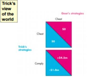
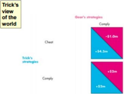
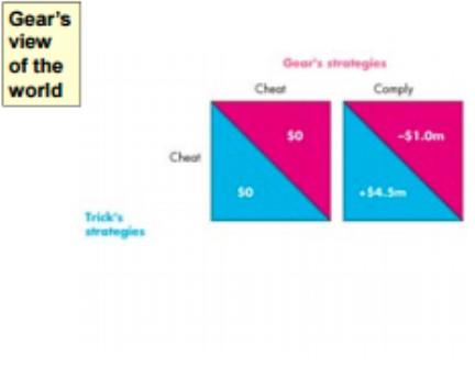
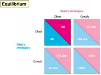
111

112 Nash Equilibrium in the Duopolists' Dilemma The Nash equilibrium is that both firms cheat The quantity and price are those of a competitive market, and firms make zero economic profit Other oligopoly games include advertising and research and development (R&D) games. These games are also prisoners' dilemmas. For example, and R&D Game in the Market for Tissues Anti-Viral Kleenex and Puffs Plus Lotion weren't developed because Kimberly-Clark (Kleenex) and P&G (Puffs) were thinking about helping you cope with a miserable cold These tissues and other innovations in the quality of facial tissues are the product of a costly R&D game. A Game of Chicken: An economic game of chicken can arise when R&D creates a new technology that cannot be patented. Both firms can benefit from the R&D of either firm. Suppose that either Apple or Nokia spends $9 million developing a new touch-screen technology that both would end up being able to use, regardless of which firm spends the $9 million

113 The equilibrium of this R&D game of chicken is for one firm to do the R&D. But we cannot tell which firm will do the R&D and which will not, Repeated Games and Sequential Games A Repeated Duopoly Game: If a game is played repeatedly, it is possible for duopolists to successfully collude and make a monopoly profit If the players take turns and move sequentially, many outcomes are possible Also additional punishment strategies enable the firms to comply and achieve a cooperative equilibrium, in which the firms make and share the monopoly profit One possible punishment strategy is a tit-for-tat strategy. A tit-for-tat strategy is one in which one player cooperates this period if the other player cooperated in the previous period but cheats in the current period if the other player cheated in the previous period A move severe punishment strategy is a trigger strategy A trigger strategy is one in which a player cooperates if the other player cooperates but plays the Nash equilibrium strategy forever thereafter if the other player cheats. A tit-for-tat strategy is sufficient to produce a cooperate equilibrium in a repeated duopoly game. Games and Price Wars: Price wars might result from a tit-for-tat strategy where there is an additional complication uncertainty about changes in demand A fall in demand might lower the price and bring forth a rough of tit-for-tat punishment

114 A Sequential Entry Game in a Contestable Market: In a contestable market a market in which firms can enter and leave so easily that firms in the market face competition from potential entrants firms play a sequential entry game In the first stage, Agile decides whether to set the monopoly price or the competitive price. In the second stage, Wannabe decides whether to enter or stay out. Wannabe's payoffs are in blue and Agile's are in red. The equilibrium is Agile sets a competitive price and makes zero economic profit to keep Wanabe out A less costly strategy is limit pricing, which sets the price at the highest level that is consistent with keeping the potential entrant out. Anti-Combine Law Canada's Anti-Common Law: Canada's first anti-combine law was enacted in 1989 The law today is defined in the competition act of 1986 The 1986 Act established a Competition Bureau and a Competition Tribunal The Act distinguishes between criminal and noncriminal practices.

115 Criminal practice include: 1. Conspiracy to fix prices 2. Bid-rigging 3. False advertising Noncriminal practices include: 1. Mergers 2. Abuse of dominant position 3. Exclusive dealing Some Major Anti-Combine Cases NutraSweet: tried to gain a monopoly in aspartame (non-sugar sweetener) by licensing the use of its swirl only on products for which it had an exclusive deal Bell Canada Enterprises: Bell Canada tried to tie the sale of advertising space in the Yellow Pages to the sale of advertising services from one of its own subsidiaries Other recent cases: Cineplex Galaxy Famous Players merge allowed Bank merger between Royal Bank and Bank of Montreal and merger between CIBC and TD Bank were blocked Gasoline price-fixing cartel in Quebec investigated and fined more than $2 million NHL cleared of anticompetitive policies

116 Chapter 16 Externalities Externalities in Our Lives An externality is a cost or benefit that arises from production and falls on someone other than the person or the firm choosing the action. A negative externality imposes a cost and a positive externality creates a benefit. The four types of externality are: 1. Negative production externalities 2. Positive production externalities 3. Negative Consumption externalities 4. Positive Consumption externalities Negative Production Externalities: Negative production externalities are common Burning coal to generate electricity emits carbon dioxide Logging and clearing forests destroys the habitat of wildlife and adds carbon dioxide to the atmosphere. Other examples are noise from aircraft and trucks, pollution of rivers and lakes, and air pollution in major cities from auto exhaust Positive Production Externalities: Positive production externalities are less common than negative externalities Two examples arise in honey and fruit production By locating honeybees next to a fruit orchard, fruit growers gets an external benefit from the bees, which pollinate the fruit orchards and boost fruit output Honey producers get an external benefit from the orchards. Negative Consumption Externalities: Negative consumption externalities are a common part of everyday life Smoking tobacco in a confined space poses a health risk to others. Noisy parties or loud car stereos disturb others or cellphone ringing in class. Positive Consumption Externalities: Positive consumption externalities are also common. When you get a flu vaccination, everyone you come into contact with benefits When the owner of an historic building restores it, everyone who sees the building gets pleasure Negative Externalities: Pollution Private, External, and Social Cost A private cost of production is a cost that is borne by the producer of a good or service Marginal private cost (MC) is the private cost of producing one more unit of a good or service An external cost of production is a cost that is NOT borne by the producer but borne by other people Marginal external cost is the cost of producing one more unit of a good or service that falls on people other than the producer. Marginal social cost (MSC) is the marginal cost incurred by the entire society by the producer and by everyone else on whom the cost falls Marginal social cost is the sum of marginal private cost and marginal external cost: MSC = MC + Marginal external cost We express costs in dollars but remember that the dollars represent the value of a forgone opportunity Marginal private cost, marginal external cost, and marginal social cost increase with output

117 Valuing an External Cost Suppose that there are two similar rivers, one polluted and the other clean with 10 identical riverside homes. The homes on the clean river rent for 2,000 a month, and those on the polluted river rent for 1,500 a month If the pollution is the only detectable difference between the houses, then the rent difference of $500 per month is the pollution cost per home. With 10 homes on the side of a polluted river, the external cost of pollution is 5,000 a month. External cost and Output: Illustrates the MC curve, the MSC curve, and marginal external cost as the vertical distance between the MC and MSC curves Equilibrium and Amount of Pollution: In the market for a good with an externality that is unregulated, the amount of pollution created depends on the equilibrium quantity of the good produced. Shows the equilibrium in an unregulated market with an external cost. The quantity of the good produced is where the marginal private cost (MC) equals marginal social benefit (MSB) At the market equilibrium, MSB is less than MSC, so the market produces an inefficient quantity of the good At the efficient quantity of the good, MSC = MSB With no regulation the market produces too much of the good and creates a deadweight loss. Three approaches to overcoming the inefficiency are: 1. Establish Property rights 2. Mandate clean technology 3. Tax or price pollution

118 Establish Property Rights: Property rights are legally established titles to the ownership, use, and disposal of factors of production and goods and services that are enforceable in the courts. Establishing property rights can confront producers with the costs of their actions and provide the incentives that allocate resources efficiently Producers with property rights have two possible responses: 1. Use an abatement technology 2. Produce less and pollute less Using an Abatement Technology An abatement technology is a production technology that reduces or prevents pollution. The producer considers alternative technologies and adopts the least-cost alternative. Produce Less and Pollute Less: An alternative to using abatement technology is to cut production and pollute less. By cutting pollution, the firm gets a higher income from renting homes on the river The decision turns on costs and the firm will choose the lest-cost alternative Efficient Market Equilibrium: Illustrates how property rights achieve an efficient outcome. The producer of the good bears all the costs So the MSC curve includes the cost of producing paint PLUS either the abatement cost or the cost of pollution The supply curve is the curve S = MC = MSC The market outcome is efficient because at the quantity of paint produced MSC equals MSB The producer bears the cost of pollution or abatement. The Coase Theorem: The Coase theorem is a proposition that if property rights exist, only a small number of parties are involved, and transactions costs are low, then private transactions are efficient. There are no externalities because all parties take into account the externalities involved The outcome is independent of who has the property rights. The Coase solution works only if transactions costs are LOW Transactions costs are the cost of conducting a transaction For example, the transactions costs of buying a home include fees for an agent, a mortgage loan advisor, and legal assistance When a large number of people are involved in an externality and transactions costs are high, the Coase solution of establishing property rights doesn't work and governments try to deal with the externality

119 Mandate Clean Technology: When property rights are too difficult to define and enforce, public choices are made. Regulation is the government's likely response. Tax or Cap and Price Pollution: Two main methods that the government uses to cope with external costs: 1. Taxes 2. Cap-and-trade Taxes: The government can set a tax equal marginal external cost The effect of such a tac is to make marginal private cost plus the tax equal to marginal social cost, MC + tax = MSC This tax is called Pigovian tax, in honor of the British economist Arthur Cecil Pigou, who first proposed dealing with externalities in this fashion How a pollution tax equal to the marginal external cost can achieve an efficient outcome. At the quantity of the good produced, MSC + MSB The government collect a tax revenue. Cap-and-Trade: A cap is an upper limit each firm is set a pollution quota A government that uses this method must first estimate the efficient quantity of pollution and set the overall cap equal to that quantity In the efficient allocation of pollution quotas, each firm has the same marginal social cost To make an efficient allocation, the government needs to know each firm's marginal cost of production and marginal abatement cost. The government solves the allocation problem by making an initial distribution of the cap across firms and allowing them to trade in a market for pollution permits. Firms with low abatement costs sell permits and make big cuts in pollution Firms with high abatement costs buy permits and make smaller cuts, or no cuts, in pollution The market price of a permit confronts polluters with the marginal social cost of their actions and leads to an efficient outcome A cap-and-trade can achieve the same efficient outcome as a Pigovian tax. Coping with Global Externalities: Canada has made its own air cleaner by adopting the measures you've just seen. But to solve the global warming problem requires public choices at a global level A lower CO2 concentration in the world's atmosphere is a global public good. And like all public goods, it brings a free-rider problem Carbon reduction also faces carbon leakage-- a tendency for non-participants in carbon reduction to increase emissions.

120 The only major attempt at international coordination of carbon reduction is the Kyoto Protocol, signed by 37 countries, not ratified by the United States, and renounced by Canada. Some governments (British Columbia in Canada and Ireland) have introduced a carbon tax Some governments (the United Kingdom) have the equivalent of a partial carbon tax on gasoline Without a mechanism to compel participation in a global carbon reduction program, contries have an incentive to leave the task to others. Positive Externality: Knowledge Private Benefits and Social Benefits A private benefit is a benefit that the consumer of a good or service receives, and marginal private benefit (MB) is the private benefit from consuming one more unit of a good or service An external benefit is a benefit that someone other than the consumer receives. Marginal external benefit is the benefit from consuming one more unit of a good or service that people other than the consumer enjoy. Marginal social benefit is the marginal benefit enjoyed by the entire society by the consumer and by everyone else on whom the benefit falls Marginal social benefit is the sum of marginal private benefit and marginal external benefit. That is: MSB = MB + Marginal external benefit Illustrates the marginal private benefit, marginal external benefit, and marginal social benefit. It identifies marginal external benefit as the vertical distance between the MB and MSB curve Shows how a private market underproduces an item that generates an external benefit... and creates a deadweight loss Government Action in the Face of External Benefits: Four devices that the government can use to achieve a more efficient allocation of resources in the presence of external benefit are: 1. Public production 2. Private subsidies 3. Vouchers 4. Patents and Copyrights

121 Public Production Under public production, a public authority that receives payment from the government produces the good or service Shows how public production can achieve an efficient outcome. Private Subsidies: A subsidy is a payment by the government to private producers If the government pays the producer an amount equal to the marginal external benefit for each unit produced, the quantity produced is efficient. Shows how a subsidy can achieve an efficient outcome: Vouchers: A voucher is a token that the government provides to households, which they can use to buy specified goods or services Shows how vouchers can achieve a more efficient outcome Patents and Copyrights: Intellectual property rights give the creator of knowledge the property right to the use of that knowledge The legal device for establishing an intellectual property right is the patent or a copyright A patent or copyright is a government-sanctioned exclusive right given to an inventor of a good, service or productive process to use to produce, use and sell the invention for a given number of years

122 Chapter 17 Public Goods and Common Resources Classifying Goods and Resources: Goods, services and resources differ in the extent to which people can be excluded from consuming them and in the extent to which one person's consumption rival other people's consumption Goods, services, and resources can be classified according to whether they are excludable or non-excludable and rival or non-rival. Excludable: A good is excludable if only the people who pay for it are able to enjoy its benefits Brink's security services, Aquaculture's Farm fish, and a Coldplay concert are examples A good is non-excludable if it is impossible (or extremely costly) to prevent anyone from benefiting from it. The service of the police, fish in the Pacific Ocean, and a concert on network television are examples Rival: A good is rival if one person's use of it decreases the quantity available for someone else A Brink's truck can't deliver cash to two banks at the same time. A fish can be consumed only once. A good is non-rival if one person's use of it does not decrease the quantity available for someone else. The services of the police and a concert on network television are non-rival A Four-Fold Classification Private Goods: A private good is both rival and excludable. A can of Coke and a fish on Aquaculture's Farm are examples of private goods Public Goods: A public good is both non-rival and non-excludable. A public good can be consumed simultaneously by everyone, and no one can be excluded from its benefits National defence is the best example of a public good. Common Resources: A common resource is rival and non-excludable. A unit of a common resource can be used only once, but no one can be prevented from using what is available. Ocean fish are a common resource. They are rival because a fish taken by one person isn't available for anyone else. They are non-excludable because it is difficult to prevent people from catching them Natural Monopoly Goods A natural monopoly good is non-rival and excludable A special case of natural monopoly arises when the good or service can be produced at zero marginal cost. Such a good is non-rival. If it is also excludable, it is produced by a natural monopoly The Internet and cable television are examples.

123 Public Goods Why does the government provide weather forecasting? Why don;t we buy it in the marketplace, as we buy hamburgers? The answer is: Weather forecasting is a public good and has a free-rider problem The Free-Rider Problem: A free-rider enjoys the benefits of a good or service without paying for it Because no one can be excluded from the benefits of a public good, everyone has an incentive to free ride Public goods create a free-rider problem A free-rider problem is that the market would provide an inefficient quantity of the public good. Marginal social benefit from a public good would exceed its marginal social cost and a deadweight loss would be created Liz and Max the only people is an imagined society value for weather forecasts The value of private good is the maximum amount that a person is willing to pay for one more unit of it The value of a public is the maximum amount that all the people are willing to pay for one more unit of it. To calculate the value placed on a public good, we use the concepts of total benefit and marginal benefit. Marginal Social Benefit of a Public Good: Total benefit is the dollar value that a person places on a given quantity of a good The greater the quantity of a good, the larger is a person's total benefit Marginal benefit is the increase in total benefit that results from a one-unit increase in the quantity of a good. The marginal benefit of a public god diminishes with the quantity of the good provided. Shows that the marginal social benefit of a public good is the sum of marginal benefits of everyone at EACH quantity of the good provided Part (a) shows Lisa's marginal benefit Part (b) shows Max's marginal benefit (c) The economy's marginal social benefit of a public good is the sum of the marginal benefits of all individuals at each quantity of the good provided. The economy's marginal social benefit curve for a public good is the vertical sum of all the individual marginal benefit curves The marginal social benefit curve for a public good contrasts with the demand curve for a private good, which is the horizontal sum of the individual demand curves at each price.

124 The Marginal Social Cost of a Public Good: The marginal social cost of a public good is determined in the same way as that of a private good. The Efficient Quantity of a Public Good: The efficient quantity of a public good is the quantity that at which marginal social benefit equals marginal social cost. Illustrates the efficient quantity of a public good With fewer than 2 weather satellites, MSB exceeds MSC Resources a can be used more efficiently by increasing the quantity With more than 2 weather satellites, MSC exceeds MSB Resources can be used more efficiently if fewer satellites are provided So the quantity at which MSB = MSC, resources are used efficiently Private production would produce 0 satellites Inefficient Private Provision: If a private firm tried to produce and sell a public good, almost no one would buy it. The free-rider problem results in too little of the good being produced. Efficient Public Provision: Because the government can tax all the consumers of the public good and force everyone to pay its provision, public provision overcomes the free-rider problem If two political parties compete, each is driven to propose the efficient quantity of a public good A party that proposes either too much or too little can be beaten by one that proposes the efficient amount because more people vote for an increase in net benefit Illustrates the efficient political outcome. Two parties, Blue and Greens, agree on everything except the number of satellites If Blues propose 1 satellite and Greens propose 3, voters are equally unhappy and the election is too close call. If Blues increase the number of satellites to 2, it will win the election if Green proposes 3. If Greens decrease the number of satellites to 2, it will win the election if Blues propose 1. Both parties propose 2 satellites and each part gets 50 percent of the votes.

125 Principle of Minimum Differentiation: The attempt by politicians to appeal to a majority of voters leads them to the same policies an example of the principle of minimum differentiation The principle of minimum differentiation is the tendency for competitors to make themselves similar so as to appeal to the maximum number of clients (voters) (The same principle applies to competing firms such as Tim Horton's and Starbucks) Inefficient Public Overprovision: If competition between two political parties is to deliver the efficient quantity of a public good, bureaucrats must cooperate and help achieve this outcome. Objective of Bureaucrats Bureaucrats want to maximize their department's budget A bigger budget increases their status and power Bureaucrats might try to persuade politicians to provide more than the efficient quantity Rational Ignorance: Rational ignorance is the decision by a voter not to acquire information about a policy or provision of a public good because the cost of doing so exceeds the expected benefit. For voters who consume but don't produce a public good, it is rational to be ignorant about the costs and benefit. For voters who produce a public good, it is rational to be well informed. When the rationality of uninformed voters and special interest groups is taken into account, the political equilibrium results in overprovision of a public good. Shows bureaucrats overprovision If rationally ignorant voters enable the bureaucrats to achieve their goal of maximizing their budget,... public good might be overprovided and... and a deadweight loss created. Two Types of Political Equilibrium: The two types of political equilibrium efficient provision and inefficient overprovision of public goods correspond to two theories of government: 1. Social Interest theory predicts that political equilibrium achieves efficiency because wellinformed voters refuse to support inefficient policies 2. Public Choice Theory predicts that government delivers an inefficient allocation of resources that government failure parallels market failure. Why Government is Large and Growing: Two possible reasons are: 1. Voter preferences 2. Inefficient overprovision Government grows because the voters' demand for some public goods is income elastic Inefficient overprovision might explain the size of government but not its growth rate

126 Voters Strike Back: If government grows too large relative to the value voters place on public goods, there might be a voter backlash, that leads politicians to propose smaller government Privatization is one way of coping with overgrown government and is based on distinguishing between public provision and public production of public goods Common Resources Overgazing the pastures around villages in Middle-age England and overfishing the cod stocks of the North Atlantic Ocean during the recent past are tragedies of the commons The tragedy of the commons is the absence of incentives to prevent the overuse and depletion of a commonly owned resource Examples include the Atlantic Ocean cod stocks, South Pacific whales, and the quantity of the earth's atmosphere The traditional example from which the term derives is the common grazing land surrounding middle-age villages Unsustainable Use of Common resource: Many common resources are renewable they replenish themselves by the birth and growth of new members of the population A common resource is being used unsustainably if its rate of use persistently decreases its stock A common resource is being used sustainably if its rate of use is less than or equal to its rate of renewal so that the stock either grows or remains constant Illustrates the sustainable catch curve SCC. As the stock of fish increases to a maximum. As the stock increases further, the fish must compete for food and the sustainable catch falls. If the catch is less than the sustainable catch at a given stock, such as point Z, the fish stock grows. If the catch exceeds the sustainable catch at a given stock, such as point A, the fish stock shrinks. The SCC shows the sustainable catch and unsustainable catch for a given stock that keeps the stock unchanged

127 The Overuse of a Common Resource Shows why overfishing occurs. The supply curve is the marginal private cost curve, MC the demand curve is the marginal social benefit curve, MSB Market equilibrium occurs at 800,000 tonnes per year and $10 a kilogram The marginal social cost curve is MSC The efficient quality is 300,000 tonnes per year At the market equilibrium, there is overfishing and a deadweight loss arises Achieving an Efficient Outcome: It is harder to achieve an efficient use of a common resource than to define the conditions under which it occurs. The three main methods use to achieve the efficient use of a common resource are : 1. Property rights 2. Production quotas 3. Individual transferable quotas (ITQs) Property rights: By converting the common resource to private property, fishers face the full social cost of their actions, The marginal social cost curve becomes the supply curve and the resource is used efficiently Production Quotas: By setting a production quota at the efficient quantity, the resource might be used efficiently Shows the profit on the marginal tonne of fish A fisher who cheats will increase his profit. There is an incentive to overfish Individual Transferable Quotas An individual transferable quota (ITQs) is a production limit that is assigned to an individual who is free to transfer (sell) the quota to someone else. A market in ITQs emerges If the efficient quantity of ITQs is assigned, the market price of an ITQ confronts resource users with a marginal cost equal to MC + price of ITQ

128 With MC + price of ITQ equal to MSB, the quantity produced is efficient Shows the situation with an efficient number of ITQs The market price of an ITQ increases the marginal social cost to MC + price of ITQ Users of the resource make MSB equal MC + price of ITQ, and the outcome is efficient.

129 Chapter 18 Markets for Factors of Production The Anatomy of Factor Markets Four factors of production are: 1. Labour 2. Capital 3. Land (natural resources) 4. Entrepreneurship Let's take a look at the markets in which these factors of production are traded. Market for Labour Services: Labour services are the physical and mental work effort that people supply to produce goods and services. A labour market is a collection of people and firms who trade labour services The price of labour services is the wage rate Most labour markets have many buyers and many sellers and are competitive. In these labour markets, the wage rate is determined by supply and demand. Market for Capital Services: Capital consists of the tools, instruments, machines, buildings, and other constructions that have been produced in the past and that businesses now use to produce goods and services These physical objets are capital goods and capital goods are traded in goods markets. This market is NOT a market for capital services A market FOR capital services is a rental market a market in which the services of capital are hired. Market for Land Services and Natural Resources: Land consists of all the gifts of nature natural resources. The market for land as a factor of production is the market for the services of land the use of land. The price of the services of land is a rental rate Nonrenewable natural resources are resources that be used only once, such as oil, natural gas, and coal. The prices of nonrenewable natural resources are determined in global commodity markets. Entrepreneurship: Entrepreneurship services are not traded in markets. Entrepreneurs receive the profit or bear the loss that results from their business decisions. The Demand for a Factor of Production The demand for a factor of production is a derived demand it is derived from the demand for the goods that it is used to produce The quantities of factors of production demanded are a consequence of firms' output decisions A firm hires the quantities of factors of production that maximize its profit The value to the firm of hiring one more unit of a factor of production is called the value of marginal product. Value of Marginal Product: The value to the firm of hiring one more unit of a factor is called its value marginal product Value of marginal product of a factor = (Price of a unit of output)(marginal product of the factor) Shows the calculation of VMP From the firm's total product schedule, calculate the marginal product of labour VMP equals marginal product of labour multiplied by the market price of the good produced.

130 A Firm's Demand for labour: The value of the marginal product of labour (VMP) tells us what an additional worker is worth to a firm VMP tells us the revenue that the firm earns by hiring one more worker. The wage rate tells us what an additional worker costs a firm VMP and the wage rate together determine the quantity of labour demanded by a firm The firm maximizes its profit by hiring the quantity of labour at which VMP = the wage rate If VMP exceeds the wage rate, the firm increase profit by employing one more worker If VMP is less than the wage rate, the firm can increase profit by firing one worker Only if VMP equals the wage rate is the firm maximizing profit Shows the relationship between a firm's value of marginal product and its demand for labour, The bars show the value of marginal product, which diminished as the quantity of labour employed increases. The value of marginal product curve passes through the midpoints of the bars The VMP of the 3 rd worker is $10 an hour So at the wage rate of $10 an hour, the firm hires 3 workers on its demand for labour curve Changes in a Firm's Demand for Labour: The firm's demand for labour depends on: 1. The price of the firm's output 2. The prices of other factors of production 3. Technology The Price of the Firm's Output: The higher the price of a firm's output, the grater is the firm's demand for labour The price of output affects the demand for labour through its influence on the value of marginal product of labour If the price of the firm's output increases, the demand for labour increases and the demand for labour curve shifts rightward.

131 The Price of Other Factors of Production If the price of using capital decreases relative to the wage rate, a firm substitutes capital for labour and increases the quantity of capital it uses. Usually, the demand for labour will decrease when the price using capital falls. Technology: New technologies decrease the demand for some types of labour and increase the demand for other types For example, if a new automated bread-making machine becomes available, a bakery might install one of these machines and fire most of its workforce a decrease in the demand for bakery workers But the firms that manufacture and service automated bread-making machines hire more labour, so there is an increase in demand for this type of labour Labour Markets A Competitive Labour Market: A market in which many firms demand labour and many household supply labour Market Demand for Labour: The market demand or labour is obtained by summing the quantities of labour demanded by all firms at each wage rate Because each firm's demand for labour curve slopes downward, so does the market demand curve The Market Supply of Labour An Individual's Labour Supply Decision: People allocate their time between leisure and labour and this choice, which determines the quantity of labour supplied, depends on the wage rate A person's reservation wage is the lowest wage rate for which he or she is willing to supply labour As the wage rate rises above the reservation wage, the household changes the quantity of labour supplied Jill's Supply of labour curve: At $5 an hour, Jill supplies NO labour, At $10 an hour, Jill supplies 30 ours of labour At $25 an hour, Jill supplies 40 hours of labour. Jill's supply labour curve is a backward bending.

132 Substitution Effect: At wage rates below $25 an hour, the higher the wage rate the greater is the quantity of labour that Jill supplies The wage rate is Kill's opportunity cost of leisure The substitution effect describes how a person responds to an increasing opportunity cost of leisure The person reduces the amount of leisure and increases the quantity of labour supplied Income Effect: The higher the wage rate, the greater is Jill's income An increase in income enables the consumer to buy more of most goods Leisure is a normal good, and the income effect describes how a person responds to a higher wage rate. The person increases the quantity of leisure and decreases the quantity of labour supplied Individual's Supply of Labour Curve: At low wage rates the substitution effect dominates the income effect, so a rise in the wage rate increases the quantity of labour supplied. At high wage rates the income effect dominates the substitution effect, so a rise in the wage rate decreases the quantity of labour supplied The labour supply curve slopes upward at low wage rates but eventually bends backward at high wage rates Market Supply Curve: A market supply curve shows the quantity of labour supplied by all households in a particular job market The market supply curve is the horizontal sum of the individual supply of labour curves Along the supply curve in a particular job market, the wage rates available in other job markets remain the same Despite the fact that an individual's labour supply curve eventually bends backward, the market supply curve of labour slopes upward Competitive Labour Market Equilibrium: Labour market equilibrium determines the wage rate and the number of worker employed Differences and Trends in Wage Rates: Wage rates increase over time trend upward because the value of marginal product of labour trends upward Technological change and the new types of capital that it brings make workers more productive With greater labour productivity, the demand for labour increases and so does the average wage rate Wage rates have become increasingly unequal High wage rates have increased rapidly while low wage rates have stagnated or even fallen.

133 A Labour Market with a Union A labour Union is an organized group of workers that aims to increase wages and influence other job conditions Influences on Labour Supply: One way to raise the wage rate is to decrease the supply of labour Influences on Labour Demand: Another way to raise the wage rate is to encourage people to buy goods produced by union workers, which raises the price of those goods and increases VMP of the workers. Labour Market Equilibrium with a Union: Unions try to restrict the supply for union labour and raise the wage rate But this action also decreases the quantity of labour demanded. So the Union tries to increase the demand for labour. Monopsony in the LabourMarket: A monopsony is a market with just one buyer. Decades ago, large manufacturing plans, steel mills, and coal mines were often the sole buyer of labour in their local labour markets Because a monopsony controls the labour market, it has the market power to set the market wage rate. Today, in some isolated parts of the country, a large mining company is the major employer. Like all firms, the monopsony has a downward-sloping demand for labour curve. The supply curve of labour tells us lowest wage rate of which a given quantity of labour is willing to work Because of the monopsony controls the wage rate, the marginal cost of labour exceeds the wage rate The marginal cost of labour curve MCL is upward slopping The monopsony maximizes profit by hiring the quantity of labour which MCL = VMP The monopsony pays the lowest rate for which the quantity of labour will work Compared to a competitive market, the monopsony employs fewer workers and pays a lower wage rate

134 A Union and a Monopsony: Sometimes both the firm and the employees have market power when a monopsony encounters a labour union, a situation called a bilateral monopoly Both the employer and the union must judge each others market power and come to an agreement on the wage rate paid and the number of workers employed Depending on the relative costs that each party can inflict on the other, the outcome of this bargaining might favor either the union or the firm Monopsony and the Minimum Wage: The imposition of a minimum wage might actually increase the quantity of labour hired by a monopsony Suppose that the minimum wage is set at $15 an hour. The minimum wage makes the supply curve of labour perfectly elastic over the range workers So over the range 0 to 150 workers, the marginal cost of hiring an additional worker equals the minimum wage For more than 150 workers, the supply of labour curve is S and the marginal cost of labour curve is MCL As a result of the minimum wage, the monopsony increases the quantity of labour employed and pays a higher wage rate than if the minimum wage were not imposed Capital and Natural Resource Markets Capital Rental Markets: The demand for capital is derived from the value of marginal product of capital Profit-maximizing firms hire the quantity of capital services that makes the value of marginal product of capital equal to the rental rate of capital Rent-Versus-Buy Decision: The cost of the services of the capital that a firm owns and operates itself is an implicit rental rate that arises from depreciation and interest costs. The decision to obtain capital services in a rental market rather than buy capital and rent it implicitly is made to minimize cost

135 Land Rental Market: The demand for land is based on the value of marginal product of land Profit-maximizing firms rent the quantity of land at which the value of marginal product of land is equal to the rental rate of land Nonrenewable Natural Resource Markets: The nonrenewable natural resources are oil, gas, and coal and these resources are traded in global commodity markets Demand and supply determine the prices and the quantities traded in these commodity markets The Demand for Oil: Two key influences on the demand for oil are: 1. The value of marginal product of oil 2. The expected future price of oil The value of marginal product of oil used, the smaller is the value of marginal product of oil Demand for oil slopes downward The higher the expected future price of oil, the greater the present demand for oil The expected future price is a speculative influence on demand A trader might buy oil to hold and sell it later for a profit-maxiinstead of buying oil to hold and sell later, the trader could buy a bond and earn interest. The opportunity cost of holding an inventory of oil is the forgone interest rate. The Supply of Oil Three key influences on the supply of oil are: 1. The known reserves 2. The scale of current oil production facilities 3. The expected future price of oil Known reserves is the oil that has been discovered and can be extracted with today's technology the greater the size of the known reserves, the greater supply of oil. The scale of current oil production facilities is the fundamental influence on supply The increasing marginal cost of extracting oil means that the supply curve of oil slopes upward The higher the price of oil, the greater is the quantity supplied Speculative forces based on expectations about the future price also influence the supply of oil The higher the expected future price of oil, the smaller is the present supply of oil A trader with an oil inventory might plan to sell now or to hold and sell later. The opportunity cost of holding the oil is the forgone interest rate. If the price of oil is expected to rise by a bigger percentage than the interest rate, it is profitable to incur the opportunity cost of holding oil rather than selling it immediately

136 Equilibrium Price of Oil: VMP of oil is the fundamental determinant of demand The marginal cost of extraction, MC, is the fundamental determinant of supply Together, they determine the market fundamentals price. If expectations about the future price of oil depart from what the market fundamentals imply, speculation can drive a wedge between the equilibrium price and the market fundamentals price. The Hotelling Principle: Hotelling Principle: the idea that traders expect the price of a nonrenewable natural resource to rise at a rate equal to the interest rate. If the price of oil is expected to rise at a rate that exceeds the interest rate, it is profitable to hold a bigger inventory, Demand increases, supply decreases, and the price rises. If the interest rate exceeds the rate at which the price of oil is expected to rise, it is not profitable to hold an oil inventory Demand decreases, supply increases, and the price falls. But if the price of oil is expected to rise at a rate equal to the interest rate, holding an inventory of oil is just as good as holding bonds. Demand and supply don't change; the price is constant Only when the price of oil is expected to rise at a rate equal to the interest rate is the price at its equilibrium