Policies that Help Develop Well-Functioning Markets [Market Development Policy] C. Some institutions that promote well-functioning markets:

Transcription

1 Gallagher Econ 460 February 2006 Policies that Help Develop Well-Functioning Markets [Market Development Policy] (I) Intro A. The assumptions of pure competition: 1. Large # of small firms 2. Homogeneous product 3. Perfect information 4. Free firm entry and exit B. So far, we've been in the public finance or resource econ mode of government intervention, which assumes that most sectors of the economy have well-functioning, competitive markets. But sometimes, policies must be undertaken that help establish a well-functioning market. These concerns are prominent in transition countries and developing economies. C. Some institutions that promote well-functioning markets: 1. Market information system mitigates the effect of uncertain prices (#3). 2. Futures markets and insurance allow farmers to shift risk and expand output (#3). 3. Co-ops can offset monopoly power. 4. Finance co-ops promote free firm entry and exit (#4). 5. Product grades and standards improve market information (#3). 6. Marketing orders offset risk for perishable commodities (#3).

2 Gallagher 2/7/06 Risk and Futures Markets 1. Uncertainty in agriculture: farmers must commit their inputs (land, capital ) before they know the actual price. However, they do have perceptions about the likelihood and range of prices. Economic analysis often assumes that producers have a probability distribution that defines their perceptions. Producers have expectations, which are defined by the mean of the distribution ( :). Producers also know the risk, which is defined by the or standard deviation of the distribution (F). 2. Producers prefer income stability. This is a consequence of the declining marginal utility of money and the Bernoulli principle (expected utility theorem). A. Suppose the producer is asked to choose between two sequences of corn prices (and incomes): ($2.50/bu, $2.50/bu) or ($1.00/bu, $4.00/bu). Both income sequences have the same mean. He chooses the first, stable, sequence of incomes if he does not like risk But the second sequence has a higher variance.

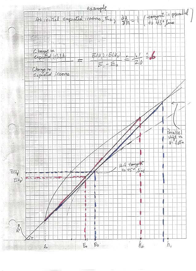
3 B. Utility under certainty is given by the utility of money function, U(M). 1. Consider an initial situation. We can choose an arbitrary utility scale. Suppose the marginal utility of money is initially $1. That is, U = $1. M o Then the value of an additional $1 is $1, initially. 2. Declining MU implies that additional $ aren't worth as much as the last dollar on the margin. C. The Bernoulli principle tells us how to value a risky prospect, or gamble, using utility theory. It says that the utility of a risky situation is the probability weighted utility of the individual outcomes (or expected utility) For example, suppose the producer finds himself stuck in an uncertain situation and he must take a gamble- the probability of low income, l, is p and the probability of the high income, h, is 1-p. So the producer s expected monetary gain, g = l D + h (1-D), is shown along the horizontal axis in the diagram. His expected utility according to the Bernoulli principle is the probability-weighted average, or expected value, of utility in the low income situation and the high income situation: Expected utility for the gamble, g, is on the straight line between U(l) and U(h) in the diagram. Specifically EU(g) is defined by the intersection with the vertical line extending through the point g. The certain income, c, has utility U(c), which lies directly on the curved utility function. In particular, the certain income c has the same utility value as the uncertain income g because U(c) and EU(g) are equal. The certain income (c) with the same utility as the uncertain income from the gamble (g) is constructed in the diagram. First, extend a horizontal line from the point [g, EU(g)] towards the vertical axis. Then read the utility. Next drop the line to the horizontal axis. Finally, the monetary amount that the producer is willing to pay to remove himself from the risky situation (insurance payment) is the amount g-c.

4 Utility: U(y) Expected Utility: E[U(y)] U(h) U(y) U(l) l c g h Income, Expected Income

5 D. Suppose a producer has initial U and declining MU m. Then he won't produce as = $1 M o much under uncertainty because higher expected income has less value under uncertainty.

6

7 3. Risk affects commodity output A. Since producers value a risky situation lower than a certain situation with the same return, they will produce less in a risky situation. The producer s effective marginal cost curve in a risky siguation, MCr, includes a risk charge-- it is higher than The MC schedule when there is no risk. For a given expected price, :, producers will produce amount Qr when there is risk and Q when there is no risk. B Remember that the lower MC schedule defines the social cost of using the last unit of resources for agricultural production. Producers should produce along this curve for efficient allocation of resources. C. The producer's welfare gain from eliminating price variability is area A+B. 4. The futures market can mitigate the adverse effects of price variability: A. A futures market is an organized exchange where buyers and sellers trade commitments for delivery of agricultural commodities. If the producer had uncertain expected price : he would evaluate marginal cost along MCr and produce output Qr. If he obtained a futures contract for post harvest delivery with the same value (:) he would evaluate marginal cost along MC and increase output to Q. B. Some argue that the futures market is efficient in the sense that the spring time futures price is an unbiased predictor of the actual cash price after harvest. There is considerable statistical evidence supporting this point for major U.S. futures markets. In other words, the market is right about the post-harvest price, on average. Consequently, producers who use futures contracts probably produce about the right

8 amount because they use the riskless marginal cost curve and use a futures price that tends to be correct about the post-harvest price. 5. What is the government role when there is a well-functioning futures market? A. There is a public good argument: 1. We've shown a producer benefit from reducing price variability F p or mitigating effects of F p with a futures market. There is a similar argument for a processor who wants to avoid a price increase. 2. The cost of developing a futures market is high for any single market participant. B. Historically though, the futures market has been a club good. That is, buyers and sellers have come together voluntarily. They buy a building and make rules for enforcing trades. C. The CFTC (Commodity Futures Trading Commission) enforces laws defined in the Commodity Exchange Act of The regulations enforced by the CFTC concern (Hieronymus, p ): 1. price manipulation 2. cheating (insider information) and fraud 3. financial standards for traders

9 Gallagher 1/28/05 Sometimes Cooperatives Countervail the Market Power of Local Processors Suppose a local processor buys milk from the local farmers along the supply curve, Sf. The processor incurs constant marginal costs Cp and receives the retail price Pr for all of the cheese that he wants to sell on the large national market. Imagine that the processor is an established producer who has his K-costs paid off; his profits are returns from cheese sales less expenses for milk and processing labor. The processor is a monopsonist (single buyer) in the local milk market. He looks at the marginal expense of input (MEI) curve when deciding how much raw milk to buy from the local farmers; and MEI curve takes the farm price increase associated with a processing expansion into account. The comparison of TEI curve and supply curve. 1) With calculus: TEI = Q m P m = Q m P m (Q m ) TEI MEI = Q m c : at a given Q = P height of supply curve m m + Q m ( + ) m P Q m slope of supply curve, MEI is higher than the supply curve(p m ) 2) Without calculus: (lbs) ($/lb) Q m P m TEI MEI /50 = /100 = /100 = /100 = /100 = /100 = /100 =

10 The monopsonist expands farm purchases until the marginal expense of the input equals the marginal revenue. In turn, the marginal revenue is the retail price less processing costs, which are given by the horizontal line Pr-Cp, in the lower diagram. So the monopoly buyer expands output to the point Qm and pays farmers the price Pm in the lower diagram. In a competitive market, output would be higher, at Qc, and the farm price would be higher, at Pr-Cp. Hence, producer returns are abnormally low and output is abnormally low, relative to the perfectly competitive ideal market. Sometimes the monopoly power is limited by the threat of entry from a cooperative processor. A new entrant will charge a capital return, Ck, with processing costs. A cooperative prices the farm input to cover costs; the payments to inputs will exactly offset the revenues from the retail market if the offer price to farmers is the retail price less processing costs less capital costs, Pr-Cp-Ck. Then farm production increases to Q1. Compared to the monopsony, the cooperative increases output, farm prices and producer profits towards the competitive level. In the United States, cooperatives cannot pay more than an 8% return on capital (usually the capital for a processing co-op is provided by the farmers). Also, retained earnings for investment do not incur corporate income tax. In contrast, income from corporations is taxed twice, once as corporate earnings, and once as stockholder dividend income. On balance, the tax break for co-ops probably reduces their required return on capital. This reduces Ck in the diagram, increases the farm price and increases the likelihood of co-op entry into the local processing market. Every time you buy (sell) something at the co-op, part of the price you pay is kept by the co-op, as a capital allowance, Ck in the diagram. This is why people say that co-ops don't work well for highly capitalized businesses. Then the co-op cost line shifts upward with capital costs, and the shift gets larger with higher capital costs..

11

12 Finance Co-ops Help Offset Capital Market Imperfections (I) Long run equilibrium at minimum AC and a zero profit rate will not occur if risk keeps the required return on capital above the normal profit rate for a competitive economy. FREE FIRM ENTRY AND EXIT IS NOT SATISFIED (See next page.) (II) Lending money can be risky with small businesses, or in a developing or a transition country. (III) Finance co-ops can pool risk and charge the average rate of return on a loan central limit theorem diversification

13 ATC: long-run average total cost D: market demand curve q i : firm output (I=0 initial situation, I=0 in long-run equilibrium) Q i : market quantity P i : market price Firm and Market Equilibrium in a Competitive Market Long-run equilibrium at minimum ATC and zero profit will not occur if risk keeps the required return on capital above the normal profit rate for a competitive economy free entry and exit is not satisfied

14 Gallagher 1/31/05 Cash Prices, Future Prices, and Inventory Equilibrium In June of the corn marketing year, supply is given by the inventory carry in from earlier in the crop year (I t-1 ). The demand curve (D(P t )) indicates the amount that will be consumed in the present, which ends when the new harvest becomes available. The inventory supply curve, ES 12, in panel b defines the amount that speculators must pay to carry grain (store inventory) into the next production period; it is defined as the difference between supply and demand at a given price. Anticipated demand and supply in the post-harvest period are shown in panel c. The demand curve D e (P e ) is a downward sloping function of the anticipated price in the post-harvest period; the anticipated price, P e, is the futures market price in the period after the crop has been planted and before the harvest is known. The demand curve represents speculators' assessment of the amount that consumers will be willing to buy next year; speculators place the position of anticipated demand based on their assessment of upcoming livestock market populations and upcoming conditions of foreign markets. Similarly, the position of the anticipated corn supply is defined by speculators collective assessment of the production for the upcoming crop. Anticipated production is indicated by the vertical line, Q a. Anticipated supply does not respond to the futures price because producers have already planted; they cannot adjust input use or output if market conditions change. The inventory demand curve in panel b, Ed a, is the difference between anticipated demand and anticipated supply at a given future price. It indicated the amount that speculators expect to receive when they sell stored inventory in the post harvest period. Equilibrium for inventory is and price is given by the intersection of the inventory supply and inventory demand schedule in panel b. The cash and futures price are equal in equilibrium; the inventory supply curve indicates the marginal cost of diverting the last unit from current consumption. Meanwhile, the inventory demand curve indicates the expected benefit from the incremental unit of future consumption. The equilibrium condition says that the two values are balanced. Finally, The futures price for the post-harvest period is what the actual cash price in the post harvest period will be IF speculators' assessment of the position of the supply and demand schedule is accurate.

15 The Effect of Inaccurate Production Forecasts First, imagine that the production forecast Q a was accurate. Then the springtime price and the post-harvest price would be the same, at P o. This would happen because the inventory carry-over, I o, would be the right amount to clear the post-harvest market at P o. Second, suppose that our estimate of production was too high; after the harvest, we find out that Q b is the amount that is actually produced even though the government announced the production forecast, Q a. The pre-harvest price is still P o because everyone expected the output forecast Q a. Similarly, I o is still the inventory carry-out because they believed the production forecast. But the actual market supply for the post-harvest period is the amount Q b + I 0. Also, the actual market price in the post harvest period (period t+1) is P t+1, which is higher than the pre-harvest futures price. Clearly, more accurate production reports would bring P t+1 and P t closer together. Hence, more accurate production forecasts stabilize prices. An improved production forecast would change the inventory decision and improve welfare. In figure 2, the best possible production forecast is Q b instead of Q a. If market participants know that Q b will occur, E db defines the expected gain from carrying inventory, and the inventory equilibrium is I 1. The improved inventory allocation also increases welfare. The welfare gain associated with changing the inventory from I 0 to I 1 is the area G in the middle diagram.

16 P t P e Q b Q a Q b +I 0 I t-1 ES 12 P e t+1 P 0 D(P t ) Ed a D e (P e ) Panel a: present supply and demand Io I 1 Panel b: inventory supply and demand I Panel c: future supply and demand Figure 1. Cash and futures Price formation with accurate production information (Q a ) and inaccurate production information (Q b )

17 P t P e Q b Q a Q b +I 1 I t-1 ES 12 G P e t+1 P 0 D(P t ) Ed d Ed a b D e (P e ) Panel a:present supply and demand Io I 1 Panel b: inventory supply and demand I Panel c: future supply and demand Figure 2. Inventory reallocation (to I 1 ) and welfare gain (G) when forecast accuracy is improved (from Q a + Q b ).

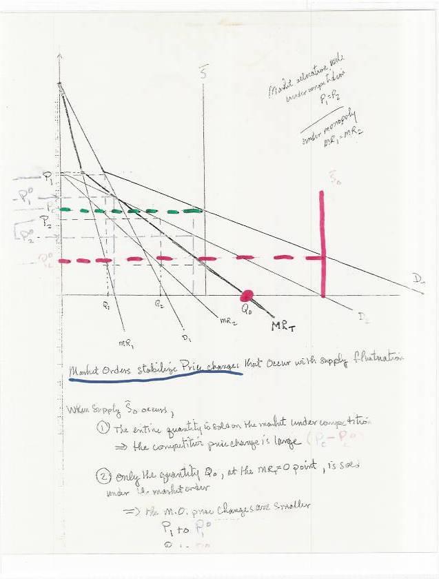
18 Marketing Orders Unregulated markets for Perishable commodities (fruits, vegetables and milk) have extreme price variability problems because: - inventories can not be carried to stabilize price fluctuations between production periods. - Low capital requirements for small producers mean large supply elasticities, for response between production periods (cobweb theorem) Futures markets are typically not highly successful for perisible commodities, because technical problems maintaining product quality make contract specification problematical. The Perishable Ag. Commodities Act provided legal sanctions for: -Grading Standards -Market Segmentation -Limitation on Quantity Marketed The Benefits of market segmentation will only occur if price discrimination can be successfully practiced. The conditions for successful Price discrimination are: -Two or more separate groups of buyers -Markets can be effectively separated by location, use, time, or type of consumer -Elasticities differ in separate markets -A large fraction of the output is sold in the high-priced market. Two diagrams below analyze the price discrimination equilibrium with a given market supply. The first diagram shows that the market order raises the average producer returns. The second diagram shows how the marketing order stabilizes supply and price fluctuations.

19

20

21 Gallagher Econ 460 January 2005 Institutions and Policies that Enhance Well-Functioning Agricultural Markets Market Failures Problems Remedy imperfect output information imperfect price information, production lag local monopsony or monopoly/ firm entry or exit - price stability - inventory carryover high/low - price risk - output low - production low - excess processor profits - publicly reported production (government agency) - futures market shifts risk (voluntary business association with government regulation) - government stabilization program (CCC) - market order for perishable crops - cooperatives operate 'at cost'. A law gives tax and antitrust exemptions in return