Course informa-on. Final exam. If you have a conflict, go to the Registrar s office for a form to bring to me

Transcription

1 Course informa-on Final exam If you have a conflict, go to the Registrar s office for a form to bring to me

2 To do today: Finish compe--on and start monopoly What it is and does: single price and price discrimina-ng monopoly What is wrong with it How can it be fixed

3

4 What if economic profit > 0? Happens because P > ATC at level of output where P (MR) = MC. What does this signal to other potential firms? How does this lead to economic profit in competition always = 0?

5

6 Adjustment if economic profit > 0

7 Characteristics of perfectly competitive equilibrium Efficient (MR = MC) Profit maximizing (MC = MR) No economic profit Lowest AC (MR = MC = AC)

8

9 Moving to the long run, when firms and enter or exit the market Part (a) illustrates the firm in long- run equilibrium..

10 Entry and exit keep economic profit = 0 in long run If supply increases, the price falls below $5 a can and Dave incurs an economic loss. Exit decreases supply to S and the price rises to $5 a can.

11 Role of entry and exit The immediate effect of the decision to enter or exit is to shift the market supply curve. If more firms enter a market, supply increases and the market supply curve shifts rightward. If firms exit a market, supply decreases and the market supply curve shifts leftward.

12 Demand also plays a role A decrease in demand triggers a similar response, except in the opposite direction. The decrease in demand brings a lower price, economic loss, and some firms exit. Exit decreases market supply and eventually raises the price to its original level.

13

14 A loss- making firm

15 Case of a loss in the short run Dave incurs an economic loss shown by the red rectangle.

16 Graphing the zero economic profit equilibrium

17 Deriving the supply curve Like the demand curve, a locus of successive equilibria For the supply curve, profit maximizing equilibria A new equilibrium every -me MR ( in perfect compe--on also the price) changes

18 Short run supply curve Increase the market price from MR 0 Get a new profit maximizing output. The new black dot in part (b) is another point of the firm s supply curve. The blue curve in part (b) is the firm s supply curve.

19 On to monopoly Main differences One firm is the whole market This means that its demand curve is downward-sloping NOT horizontal like in perfect competition

20 Main analytical differences in monopoly In perfect competition, because MR is constant, MR = AR (and remember, AR is also the price so the AR curve is also the demand curve) In monopoly, with a downward-sloping demand curve (and therefore AR curve) the MR curve is downward sloping and below the AR (pulling AR down)

21 MONOPOLY AND HOW IT ARISES No Close Substitutes If a good has a close substitute, even though only one firm produces it, that firm effectively faces competition from the producers of substitutes.

22 MONOPOLY AND HOW IT ARISES Barriers to Entry Any constraint that protects a firm from competitors is a barrier to entry. There are three types of barrier to entry: Natural Ownership Legal

23 Natural monopoly Industry with decreasing costs (economies of scale) throughout the range of demand One firm produces at the lowest cost; more firms would raise costs

24

25 Tradeoff between price and the quantity sold. To sell a larger quantity, the monopolist must set a lower price. Two price-setting possibilities that create different tradeoffs: Single price Price discrimination

26 MONOPOLY AND HOW IT ARISES Single Price A single-price monopoly is a firm that must sell each unit of its output for the same price to all its customers. DeBeers sell diamonds (quality given) at a single price.

27 MONOPOLY AND HOW IT ARISES Price Discrimination A price-discriminating monopoly is a firm that is able to sell different units of a good or service for different prices. Airlines offer different prices for the same trip.

28 Single price monopoly Central feature: downward sloping demand (AR) curve Therefore MR< AR Because to sell more, have to reduce the price on all units sold

29 SINGLE- PRICE MONOPOLY The marginal revenue curve slopes downward and is below the demand curve. Marginal revenue is less than price.

30 Elas-city and revenue again 1. If a price fall increases total revenue, demand is elas-c. 2. If a price fall decreases total revenue, demand is inelas-c.

31 Elas-city and the demand curve again Elas-city will change along the demand curve, as we have seen This means that to know the effect of a change in price, must know where you are on the demand curve

32 Elas-city and MR along the demand curve

33

34

35 SINGLE- PRICE MONOPOLY Marginal Revenue and Elas-city Recall the total revenue test, which determines whether demand is elas-c or inelas-c. 1. If a price fall increases total revenue, demand is elas-c. 2. If a price fall decreases total revenue, demand is inelas-c. Use the total revenue test to see the rela-onship between marginal revenue and elas-city.

36 Monopoly equilibrium Same profit maximizing rule: MC = MR But now, P or AR is above MR So, monopoly sells a smaller output at a higher price

37 Graphing monopoly equilibrium

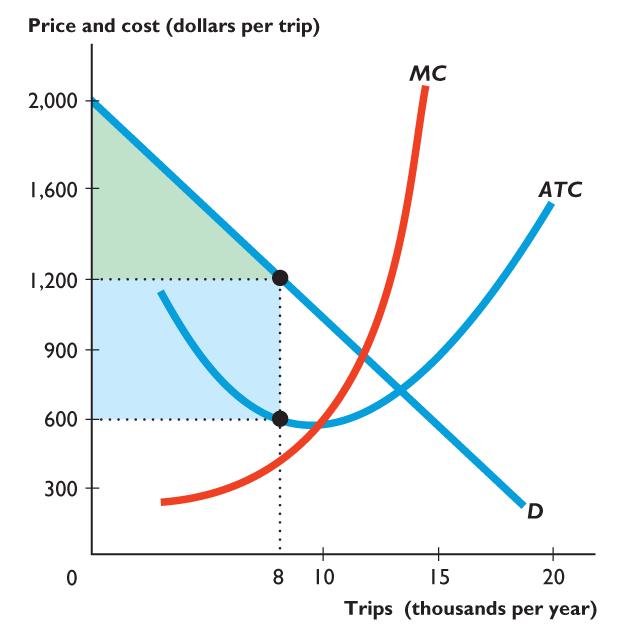
38 Full profit- maximizing story Rule: MC = MR Again same as profit maximizing rule in compe--on The average total cost curve is ATC. The marginal cost curve is MC. The demand curve is D. The marginal revenue curve is MR.

39 Characteris-cs of monopoly profit- maximiza-on Decision rule is the same as in compe--on for level of output: MR = MC But, the rest of the story is different Profit at this output is not limited to normal profit Economic profit is posi-ve!

40

41 Monopoly vs compe--on Tricky bit The price the monopoly charges at its profit maximizing output is from its DEMAND curve, like usual Not from its MR curve, which is now below the demand curve

42 Characteris-cs of monopoly Economic profit > 0 Price is higher than compe--ve level Output is less than the compe--ve level And now, have deadweight loss So monopoly is not efficient

43 Where to compare monopoly and compe--on? Perfectly compe--ve equilibrium where MC (S) = MB (price and demand curve) So, on the monopoly graph, perfect compe--ve is where S=MC curve intersects the demand curve

44 Monopoly vs compe--on

45

46 Consequences of monopoly Higher equilibrium prices Lower equilibrium quan-ty Deadweight loss (MC not = MB)

47

48 Price discrimina-ng monopoly Price discrimina-on selling a good or service at a number of different prices is widespread. To be able to price discriminate, a firm must Iden-fy and separate different types of buyers. Sell a product that cannot be resold.

49 Price discrimina-on and consumer surplus Goal: to convert consumer surplus into economic profit by charging different categories of consumers different prices Perfect price discrimina-on: each individual customer pays separate price schedule based on that customer s own willingness to pay.

50

51

52 Perfect price discrimina-on

53

54

55 Increase in economic profit from perfect price discrimina-on

56 Price discrimina-on and efficiency Price equals MC, so deadweight loss is zero But consumer surplus now all goes to producer Rent seeking becomes profitable and rent seekers use up the whole producer surplus