Process Performance and Quality Chapter 6

Transcription

1 Process Performance and Quality Chapter 6

2 How Process Performance and Quality fits the Operations Management Philosophy Operations As a Competitive Weapon Operations Strategy Project Management Process Strategy Process Analysis Process Performance and Quality Constraint Management Process Layout Lean Systems Supply Chain Strategy Location Inventory Management Forecasting Sales and Operations Planning Resource Planning Scheduling

3 Costs of Poor Process Performance Defects: Any instance when a process fails to satisfy its customer. Prevention costs are associated with preventing defects before they happen. Appraisal costs are incurred when the firm assesses the performance level of its processes. Internal failure costs result from defects that are discovered during production of services or products. External failure costs arise when a defect is discovered after the customer receives the service or product.

4 Total Quality Management Quality: A term used by customers to describe their general satisfaction with a service or product. Total quality management (TQM) is a philosophy that stresses three principles for achieving high levels of process performance and quality: 1. Customer satisfaction 2. Employee involvement 3. Continuous improvement in performance

5 TQM Wheel Customer satisfaction

6 Customer Satisfaction Customers, internal or external, are satisfied when their expectations regarding a service or product have been met or exceeded. Conformance: How a service or product conforms to performance specifications. Value: How well the service or product serves its intended purpose at a price customers are willing to pay. Fitness for use: How well a service or product performs its intended purpose. Support: Support provided by the company after a service or product has been purchased. Psychological impressions: atmosphere, image, or aesthetics

7 Employee Involvement One of the important elements of TQM is employee involvement. Quality at the source is a philosophy whereby defects are caught and corrected where they were created. Teams: Small groups of people who have a common purpose, set their own performance goals and approaches, and hold themselves accountable for success. Employee empowerment is an approach to teamwork that moves responsibility for decisions further down the organizational chart to the level of the employee actually doing the job.

8 Team Approaches Quality circles: Another name for problem-solving teams; small groups of supervisors and employees who meet to identify, analyze, and solve process and quality problems. Special-purpose teams: Groups that address issues of paramount concern to management, labor, or both. Self-managed team: A small group of employees who work together to produce a major portion, or sometimes all, of a service or product.

9 Continuous Improvement Continuous improvement is the philosophy of continually seeking ways to improve processes based on a Japanese concept called kaizen. 1. Train employees in the methods of statistical process control (SPC) and other tools. 2. Make SPC methods a normal aspect of operations. 3. Build work teams and encourage employee involvement. 4. Utilize problem-solving tools within the work teams. 5. Develop a sense of operator ownership in the process.

10 The Deming Wheel Plan-Do-Check-Act Cycle Plan Act Do Check

11 Statistical Process Control Statistical process control is the application of statistical techniques to determine whether a process is delivering what the customer wants. Acceptance sampling is the application of statistical techniques to determine whether a quantity of material should be accepted or rejected based on the inspection or test of a sample. Variables: Service or product characteristics that can be measured, such as weight, length, volume, or time. Attributes: Service or product characteristics that can be quickly counted for acceptable performance.

12 Sampling Sampling plan: A plan that specifies a sample size, the time between successive samples, and decision rules that determine when action should be taken. Sample size: A quantity of randomly selected observations of process outputs.

13 Sample Means and the Process Distribution Sample statistics have their own distribution, which we call a sampling distribution.

14 Sampling Distributions A sample mean is the sum of the observations divided by the total number of observations. Sample Mean x = n i =1 n x i where x i = observations of a quality characteristic such as time. n = total number of observations x = mean The distribution of sample means can be approximated by the normal distribution.

15 Sample Range The range is the difference between the largest observation in a sample and the smallest. The standard deviation is the square root of the variance of a distribution. where ( x) x i = σ n 1 2 σ = standard deviation of a sample n = total number of observations x i = observations of a quality characteristic x = mean

16 Process Distributions A process distribution can be characterized by its location, spread, and shape. Location is measured by the mean of the distribution and spread is measured by the range or standard deviation. The shape of process distributions can be characterized as either symmetric or skewed. A symmetric distribution has the same number of observations above and below the mean. A skewed distribution has a greater number of observations either above or below the mean.

17 Causes of Variation Two basic categories of variation in output include common causes and assignable causes. Common causes are the purely random, unidentifiable sources of variation that are unavoidable with the current process. If process variability results solely from common causes of variation, a typical assumption is that the distribution is symmetric, with most observations near the center. Assignable causes of variation are any variationcausing factors that can be identified and eliminated, such as a machine needing repair.

18 Assignable Causes The red distribution line below indicates that the process produced a preponderance of the tests in less than average time. Such a distribution is skewed, or no longer symmetric to the average value. A process is said to be in statistical control when the location, spread, or shape of its distribution does not change over time. After the process is in statistical control, managers use SPC procedures to detect the onset of assignable causes so that they can be eliminated. Location Spread Shape

19 Control Charts Control chart: A time-ordered diagram that is used to determine whether observed variations are abnormal. A sample statistic that falls between the UCL and the LCL indicates that the process is exhibiting common causes of variation; a statistic that falls outside the control limits indicates that the process is exhibiting assignable causes of variation.

20 Control Chart Examples

21 Type I and II Errors Control charts are not perfect tools for detecting shifts in the process distribution because they are based on sampling distributions. Two types of error are possible with the use of control charts. Type I error occurs when the employee concludes that the process is out of control based on a sample result that falls outside the control limits, when in fact it was due to pure randomness. Type II error occurs when the employee concludes that the process is in control and only randomness is present, when actually the process is out of statistical control.

22 Statistical Process Control Methods Control Charts for variables are used to monitor the mean and variability of the process distribution. R-chart (Range Chart) is used to monitor process variability. x-chart is used to see whether the process is generating output, on average, consistent with a target value set by management for the process or whether its current performance, with respect to the average of the performance measure, is consistent with past performance. If the standard deviation of the process is known, we can place UCL and LCL at z standard deviations from the mean at the desired confidence level.

23 Control Limits The control limits for the x-chart are: UCL x = x + A 2 R and LCL x = x - A 2 R Where = X = central line of the chart, which can be either the average of past sample means or a target value set for the process. A 2 = constant to provide three-sigma limits for the sample mean. = = The control limits for the R-chart are UCL R = D 4 R and LCL R = D 3 R where R = average of several past R values and the central line of the chart. D 3,D 4 = constants that provide 3 standard deviations (three-sigma) limits for a given sample size.

24 Calculating Three-Sigma Limits Table 6.1

25 West Allis Industries Example 6.1 West Allis is concerned about their production of a special metal screw used by their largest customers. The diameter of the screw is critical. Data from five samples is shown in the table below. Sample size is 4. Is the process in statistical control?

26 West Allis Industries Control Chart Development Example = Sample Sample Special Metal Screw Number R x _ ( )/4 =

27 Example 6.1 West Allis Industries Completed Control Chart Data Special Metal Screw Sample Sample _ Number R x R = x = =

28 R = D 4 = D 3 = 0 Example 6.1 West Allis Industries R-chart Control Chart Factors Factor for UCL Factor for Factor Size of and LCL for LCL for UCL for Sample x-charts R-Charts R-Charts (n) (A 2 ) (D 3 ) (D 4 ) UCL R = D 4 R = (0.0021) = in. LCL R = D 3 R 0 (0.0021) = 0 in.

29 Example 6.1 West Allis Industries Range Chart

30 Example 6.1 West Allis Industries x-chart Control Chart Factor Factor for UCL Factor for Factor Size of and LCL for LCL for UCL for Sample x-charts R-Charts R-Charts (n) (A 2 ) (D 3 ) (D 4 ) R = A 2 = = x = UCL x = x = + A 2 R = (0.0021) = in. LCL x = x= - A 2 R = (0.0021) = in.

31 Example 6.1 West Allis Industries x-chart Sample the process Eliminate the problem Find the assignable cause Repeat the cycle

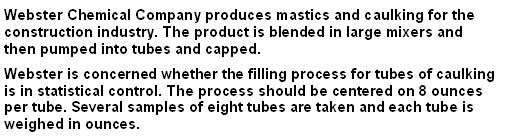
32 Application 6.1

33 Application 6.1 UCL R = D R = 1.864(0.38) = LCL R = D R = 0.136(0.38) =

34 Application 6.1 UCL R = D4 R = 1.864( 0.45) = LCL R = D3 R = 0.136( 0.45) = UCL = x + A2 R = ( 0.45) = x = x A R = ( 0.45) LCL x 2 =

35 σ x = σ/ n Sunny Dale Bank Example 6.2 Sunny Dale Bank management determined the mean time to process a customer is 5 minutes, with a standard deviation of 1.5 minutes. Management wants to monitor mean time to process a customer by periodically using a sample size of six customers. Design an x-chart that has a type I error of 5 percent. That is, set the control limits so that there is a 2.5 percent chance a sample result will fall below the LCL and a 2.5 percent chance that a sample result will fall above the UCL. Sunny Dale Bank x = = 5.0 minutes σ = 1.5 minutes n = 6 customers z = 1.96 = Control Limits UCL x = x + zσ x LCL x = x = UCL zσ x = (1.5)/ 6 = 6.20 min x LCL x = (1.5)/ 6 = 3.80 min After several weeks of sampling, two successive samples came in at 3.70 and 3.68 minutes, respectively. Is the customer service process in statistical control?

36 Control Charts for Attributes p-chart: A chart used for controlling the proportion of defective services or products generated by the process. σ p = p(1 p)/n Where n = sample size p = central line on the chart, which can be either the historical average population proportion defective or a target value. Control limits are: UCL p = p+zσ p and LCL p = p zσ p z = normal deviate (number of standard deviations from the average)

37 Hometown Bank Example 6.3 The operations manager of the booking services department of Hometown Bank is concerned about the number of wrong customer account numbers recorded by Hometown personnel. Each week a random sample of 2,500 deposits is taken, and the number of incorrect account numbers is recorded. The results for the past 12 weeks are shown in the following table. Is the booking process out of statistical control? Use three-sigma control limits.

38 Hometown Bank Using a p-chart p to monitor a process p = n = 2500 σ p = p(1 p)/n (2500) = σ p = ( )/ )/2500 σ p = UCL p = (0.0014) = LCL p = (0.0014) = Sample Wrong Proportion Number Account # Defective Total 147

39 Example 6.3 Hometown Bank Using a p-chart p to monitor a process

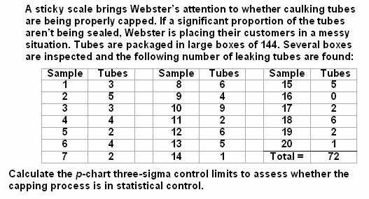
40 Application 6.2

41 Application 6.2 p = Total number of Total number leaky tubes of tubes = ( ) = σ p = p ( 1 p) 0.025( ) n = 144 = UCL p = p + zσ p = ( ) = LCL p = p zσ p = ( ) = LCL p = 0

42 c-charts c-chart: A chart used for controlling the number of defects when more than one defect can be present in a service or product. The underlying sampling distribution for a c-chart is the Poisson distribution. The mean of the distribution is c The standard deviation is c A useful tactic is to use the normal approximation to the Poisson so that the central line of the chart is c and the control limits are UCL c = c+z c and LCL c = c z c

43 Woodland Paper Company Example 6.4 In the Woodland Paper Company s final step in their paper production process, the paper passes through a machine that measures various product quality characteristics. When the paper production process is in control, it averages 20 defects per roll. a) Set up a control chart for the number of defects per roll. Use twosigma control limits. b) Five rolls had the following number of defects: 16, 21, 17, 22, and 24, respectively. The sixth roll, using pulp from a different supplier, had 5 defects. Is the paper production process in control? c = 20 z = 2 UCL c = c+z c = = LCL c = c z c = = 11.06

44 Example 6.4 Woodland Paper Company Using a c-chart to monitor a process Solver - c-charts Number of Defects Sample Number

45 Application c = = 4 σ c = 4 = 2 12 UCL c + zσ = 4 + 2( 2) = 8 LCL c zσ = 4 2( 2) = 0 c = c c = c

46 Process Capability Process capability is the ability of the process to meet the design specifications for a service or product. Nominal value is a target for design specifications. Tolerance is an allowance above or below the nominal value.

47 Process Capability Lower specification Nominal value Process distribution Upper specification Minutes Process is capable

48 Process Capability Lower specification Nominal value Process distribution Upper specification Minutes Process is not capable

49 Effects of Reducing Variability on Process Capability Nominal value Six sigma Four sigma Two sigma Lower specification Upper specification Mean

50 Process Capability Index, C pk Process Capability Index, C pk, is an index that measures the potential for a process to generate defective outputs relative to either upper or lower specifications. C pk = Minimum of x = Lower specification Upper specification x = 3σ, 3σ We take the minimum of the two ratios because it gives the worst-case situation.

51 Process Capability Ratio, C p Process capability ratio, C p, is the tolerance width divided by 6 standard deviations (process variability). C p = Upper specification - Lower specification 6σ

52 Using Continuous Improvement to Determine Process Capability Step 1: Collect data on the process output; calculate mean and standard deviation of the distribution. Step 2: Use data from the process distribution to compute process control charts. Step 3: Take a series of random samples from the process and plot results on the control charts. Step 4: Calculate the process capability index, C pk, and the process capability ratio, C p, if necessary. If results are acceptable, document any changes made to the process and continue to monitor output. If the results are unacceptable, further explore assignable causes.

53 Intensive Care Lab Example 6.5 The intensive care unit lab process has an average turnaround time of 26.2 minutes and a standard deviation of 1.35 minutes. The nominal value for this service is 25 minutes with an upper specification limit of 30 minutes and a lower specification limit of 20 minutes. The administrator of the lab wants to have four-sigma performance for her lab. Is the lab process capable of this level of performance? Upper specification = 30 minutes Lower specification = 20 minutes Average service = 26.2 minutes σ = 1.35 minutes

54 Intensive Care Lab Assessing Process Capability Example 6.5 Upper specification = 30 minutes Lower specification = 20 minutes Average service = 26.2 minutes σ = 1.35 minutes C pk = Minimum of x = Lower specification Upper specification x = 3σ, 3σ C pk = Minimum of , ) 3( ) 3(1.35 C pk = Minimum of 1.53, 0.94 = 0.94 = 0.94 Process Capability Index

55 Example 6.5 C pk = C p = Intensive Care Lab Assessing Process Capability Upper specification - Lower specification 6σ = 1.23 Process Capability Ratio (1.35) Does not meet 4σ (1.33 C p ) target Before Process Modification Upper specification = 30.0 minutes Lower specification = 20.0 minutes Average service = 26.2 minutes σ = 1.35 minutes C pk = 0.94 C p = 1.23 After Process Modification Upper specification = 30.0 minutes Lower specification = 20.0 minutes Average service = 26.1 minutes σ = 1.2 minutes C pk = 1.08 C p = 1.39

56 Application 6.4 C pk = x lower specification upper specification x min, = 3σ 3σ min = 1.135, = = 3( 0.192) 3( 0.192) 0.948

57 Application 6.4 C p upper specification lower = 6σ = 6 ( 0.192) = specification

58 Quality Engineering Quality engineering is an approach originated by Genichi Taguchi that involves combining engineering and statistical methods to reduce costs and improve quality by optimizing product design and manufacturing processes. Quality loss function is the rationale that a service or product that barely conforms to the specifications is more like a defective service or product than a perfect one. Quality loss function is optimum (zero) when the product s quality measure is exactly on the target measure.

59 Taguchi's Quality Loss Function Loss (dollars) Lower specification Nominal value Upper specification

60 Six Sigma Six Sigma is a comprehensive and flexible system for achieving, sustaining, and maximizing business success by minimizing defects and variability in processes. It relies heavily on the principles and tools of TQM. It is driven by a close understanding of customer needs; the disciplined use of facts, data, and statistical analysis; and diligent attention to managing, improving, and reinventing business processes.

61 Six Sigma Improvement Model 1. Define Determine the current process characteristics critical to customer satisfaction and identify any gaps. 2. Measure Quantify the work the process does that affects the gap. 3. Analyze Use data on measures to perform process analysis. 4. Improve Modify or redesign existing methods to meet the new performance objectives. 5. Control Monitor the process to make sure high performance levels are maintained.

62 Six Sigma Implementation Top Down Commitment from corporate leaders. Measurement Systems to Track Progress Tough Goal Setting through benchmarking best-in-class companies. Education: Employees must be trained in the whys and how-tos of quality. Communication: Successes are as important to understanding as failures. Customer Priorities: Never lose sight of the customer s priorities.

63 Six Sigma Education Green Belt: An employee who achieved the first level of training in a Six Sigma program and spends part of his or her time teaching and helping teams with their projects. Black Belt: An employee who reached the highest level of training in a Six Sigma program and spends all of his or her time teaching and leading teams involved in Six Sigma projects. Master Black Belt: Full-time teachers and mentors to several black belts.

64 International Quality Documentation Standards ISO 9000 A set of standards governing documentation of a quality program. ISO Documentation standards that require participating companies to keep track of their raw materials use and their generation, treatment, and disposal of hazardous wastes.

65 1. Category 1 Leadership 120 points 2. Category 2 Strategic Planning 85 points 3. Category 3 Customer and Market Focus 85 points 4. Category 4 Measurement, Analysis, and Knowledge Management 90 points 5. Category 5 Human Resource Focus 85 points 6. Category 6 Process Management 85 points 7. Category 7 Business Results 450 points Malcolm Baldrige National Quality Award Named after the late secretary of commerce, a strong proponent of enhancing quality as a means of reducing the trade deficit. The award promotes, recognizes, and publicizes quality strategies and achievements.