Viscoelasticity, Creep and Fiber-filled Materials

Transcription

1 Viscoelasticity, Creep and Fiber-filled Materials Hubert Lobo expert material testing CAE material parameters CAE Validation software & infrastructure for materials materials know ledge electronic lab notebooks

2 Definitions of creep and viscoelasticity Creep is the change that occurs to a material due constant load over time Depends on applied load Depends on temperature/environment Stress relaxation is the change that occurs to a material due to constant deformation over time Depends on applied strain Depends on temperature/environment Viscoelasticity is the property consisting of both elastic behavior and flow (plastic) behavior, in which time varies the behavior of each component Depends on time/frequency Depends on load/strain Depends on temperature/environment

3 Effect of temperature Properties and dependencies change with temperature Modulus Ductile-brittle transitions Rate dependency

4 Effect of environment: in-vivo Saline solution at body temperature

5 Creep behavior Primary Short time Loading phase transient Secondary Sustained uniform strain Handled by creep models Tertiary Localization and failure Creep rupture

6 Creep modeling Creep strain vs. time, fit to time hardening model Minimum 3 stress levels Typically 1000 hours Can incorporate temperate but best handled as individual models for each temperature (more stable/accurate) Plastic deformation ASTM D2990 / ISO Strain (%) MPa, 60 C, Replicate MPa, 60 C, Replicate MPa, 60 C, Replicate MPa, 60 C, Replicate MPa, 60 C, Replicate 1 c2 c MPa, 60 C, Replicate 2 C1 t cr 0.0 1E-02 1E-01 1E+00 1E+01 1E+02 1E+03 Time (Hours)

7 Modulus (MPa) Stress relaxation Stress relaxation Stress/Modulus will relax over time Logarithmic behavior Typically 1000 hours Plastic deformation ASTM D6147 1E+04 1E+03 1E+02 1E-05 1E-03 1E-01 1E+01 1E+03 Time (hrs) Log-Log Scaling Modulus (MPa) 2E+03 2E+03 2E+03 2E+03 1E+03 1E+03 9E+02 7E+02 5E+02 3E+02 1E+02 Instantaneous 0E+00 2E+02 4E+02 6E+02 8E+02 1E+03 Time (hrs) Linear-Linear Scaling Long term

8 Viscoelasticity In small strain (linear viscoelastic) situations Applied strain (stress) is recoverable Frequency or time based measurements A time-temperature correlation exists Higher temperature = longer time Lowering temperature = short time

9 DMA (dynamic mechanical analysis) operation Force or displacement control Dynamic or constant application G' (Pa) 1E+10 1E+09 1E+08 G' tan delta tan delta E+07 1.E Temperature ( C) Temperature sweep E E-02 Example of force based DMA G', G" (Pa) 1.E+07 1.E+06 G' A G" A tan d 3.5E E E E E E E-03 Derivation of dynamic modulii 1.E E Frequency (rad/s) Frequency sweep

10 TTS (time-temperature superposition) Takes advantage of both time and temperature sensitivity of material Measure frequency or time sweep at multiple temperautes Shift curves in time/freq domain Generate a mastercurve at times/freq higher than possible to test Also generate temperature sensitivity

11 Torsional mode Torsional DMA Temperature: -125 to 600 C Frequency: 0.01 to 500 rad/s Steady or dynamic modes Torque range: 2 to 2000 gm-cm Specimens 25 mm diam. Disc Torsional (flex) bar Data G -G data tan delta Shear stress relaxation

12 Tension/compression mode Dynamic tensile-compression Frequency: Hz Load: N Crosshead speed 0-3 m/s Displacement: ±12.7 mm Temperature: -80 to 250C Specimens ASTM type V tensile bar Compression cube (25mm depending on stiffness) Data E E (tensile loss/storage modulus) tan delta Tensile relaxation modulus E f(t)

13 PTFE mastercurve (stress relaxation) Caution should be exercised in using very large time scale data Environment reaction of material (deterioration of material, chemical exposure, etc.) Assumes all things are constant Beware of transition temperatures (TTS does not work) Shift factors

14 Viscoelasticity & environmental effects In-vivo stress relaxation for hip replacement material

15 Viscoelastic models Time-based Prony series Frequency-based ' G i G i G i G G " G i G i G i G G

16 Viscoelastic models Normalized modulus data fit to 6-parameter Prony series Used for simulating short or long term events Can apply WLF shift factors for different temperatures Prony series WLF equation

17 Limitations Depends on linear viscoelastic theory Can predict non-linear effects Cannot predict large strain deformation Cannot predict failure Great caution when used with hyperelasticity or other large deformation model

18 Fiber Filled Plastics and the Need for Injection Molding Simulation expert material testing CAE material parameters CAE Validation software & infrastructure for materials materials know ledge electronic lab notebooks

19 Fiber-filled plastics Spatial orientation of fibers Properties vary spatially Significant property differences with orientation Can approximate: Worst case: use cross-flow data Use third party software to map then implement orientation effects to FEA Injection molding simulation of part to capture fiber alignment Digimat or Helius to impart material properties Send to FEA Source:e-Xstream

20 Injection molding simulation Simulate injection molding process Mold design Fiber orientation Final part geometry (warp/shrink) Frozen stresses Third party software Autodesk Moldflow Moldex 3D Sigmasoft

21 Required testing Viscosity Specific heat DSC transition temperatures Thermal conductivity PVT Linear shrinkage Viscoelastic properties Mold filling Packing Post-mold Shrinkage Warpage

22 Rheometer measurement of viscosity Capillary rheometer is used Material is extruded through a restriction of known geometry (extremely high tolerance dies) Temperature and flow rate are controlled Pressure drop across the restriction is used to determine viscosity as a function of shear rate and temperature

23 Viscosity properties As shear rate increases, viscosity decreases

24 Viscosity properties As temperature increases, viscosity decreases

25 Viscosity measurements Apparent Viscosity Shear rate: Shear stress: Shear viscosity: Corrections to viscosity Reservoir and friction losses (transducer located at die) End pressure drop (Bagley) 32Q a 3 d pd w 4L w a Non-parabolic velocity (Rabinowitsch correction) a where: Q = Volume flow rate p = Pressure drop d = Capillary diameter L = Capillary length

26 Bagley correction testing Bagley correction Perform viscosity measure on two different die ratios at equal shear rates Evaluate pressure differences between die geometries (capillary diameter remains the same) = R/2(dP/dL)

27 Viscosity modeling Very strong rheological models Cross WLF, Cross Arrhenius Combines a model of shear rate dependency with temperature dependency Allows us to predict beyond testing range T, 0 T D T * 1 1n T A1 exp A 2, where D2 T D 2 n * D1 3.86E+13 D A A2 51.6

28 Specific heat DSC (differential scanning calorimeter) Small samples sizes (7-15 mg) Differential heat required to raise the temperature of the sample as compared to a reference Performed in cooling to replicate molten material cooling to solidification Used in the simulation to determine how much energy must be dissipated to promote solidification

29 Thermal conductivity A measure of how well a material transfers heat Measured using transient line source Measured in melt and solid state Different behaviors for semi-crystalline and amorphous Measure time to dissipate the heat pulse away from probe

30 Thermal conductivity Semi-crystalline materials show an increase in thermal conductivity in solid state Amorphous materials show a decrease in thermal conductivity in solid state The addition of fillers increase thermal conductivity Thermal conductivity of polymers is much lower than metals Copper: 400 W/mK ABS: W/mK

31 Density as a function of PVT (pressure, volume and temperature) Isobaric cooling scan (for semi-crystalline materials) Need to accurately capture the onset of crystallization Much longer run times Isothermal heating scan (for amorphous materials) No crystallization so transition is independent of mode Much faster (relatively) Pressures of Mpa Measure both solid and melt domains

32 PVT testing Difficult and time consuming test Initial density at ambient conditions Mercury used as confining fluid High temperatures and pressures Complex datasets True hydrostatic state

33 PVT test data Semi-crystalline material Transition region is critical Rise in temp. = rise in spec. vol. Rise in press. = drop in spec. vol. Molten Transitional Solid

34 PVT test data Amorphous material Transition is not dependent on mode Molten Solid

35 PVT modeling Two-Domain Tait PVT Model: Two-domain Tait model 13 parameters Three groups of paramters b5 is the transition of the low pressure b6 is the slope of the transition b7, b8, and b9 describe the shape of the crystalline transition b E+02 K b E-07 K/Pa b1m 1.081E-03 m 3 /kg b2m 7.707E-07 m 3 /kg K b3m 6.864E+07 Pa b4m 3.209E-03 1/K b1s 1.011E-03 m 3 /kg b2s 4.442E-07 m 3 /kg K b3s 1.397E+08 Pa b4s 1.752E-03 1/K b E-05 m 3 /kg b E-02 1/K b E-08 1/Pa

36 PVT modeling, cont. b1m is the specific volume at b5 b2m is the slope of the melt region b3m is the pressure sensitivity or spread of the melt fit b4m is the pressure sensitivity of the melt state slope b1s through b4s are the same but for the solid state Two-Domain Tait PVT Model: b E+02 K b E-07 K/Pa b1m 1.081E-03 m 3 /kg b2m 7.707E-07 m 3 /kg K b3m 6.864E+07 Pa b4m 3.209E-03 1/K b1s 1.011E-03 m 3 /kg b2s 4.442E-07 m 3 /kg K b3s 1.397E+08 Pa b4s 1.752E-03 1/K b E-05 m 3 /kg b E-02 1/K b E-08 1/Pa b2m b1m b3m

37 Thermal expansion TMA (thermo-mechanical analyzer) 10 x 10 mm x thickness plaques Low expansion quartz probe and station Constant heating rate Slope of dl over temperature Orientation One direction for no fiber Two directions for fiber-filled

38 Thermal expansion test data Data presented as calculated slopes that are constant over the test range Plot of probe position vs. temperature ensures linear relationship Anisotropic materials Measurements across the flow always higher Fibers have less thermal expansion than polymer

39 Mechanical properties Tensile tests performed on a UTM Temperature chamber Axial and transverse strains Measure only the unfilled polymer Fibers added in with the micro-mechanical model Stress strain curves at multiple temperatures Modulus (/) Poisson s ratio (2/1) Viscoelastic properties

40 Problematic Materials Moisture sensitive materials Improperly dried materials cause reduction in viscosity Over-dried materials cause a rise in viscosity PET, PA, PC, PBT etc. Highly filled materials Can log jam the die entrance Special dies must be used Higher scatter in test data requires engineering judgment on behavior Thermally unstable materials Require very careful attention to residence times PVC

41 Basic DIGIMAT MX TestPak protocol Mold 100 X 300 X 3.16mm plaques Edge gated on 100 mm end Long flow length Fully developed flow Highly fiber orientation Cut test specimens by CNC 5 specimens each (0, 90, other orientations ) Obtain true stress-strain data Calibrate material model

42 DIGIMAT MX TestPak outputs CAD drawings of plaque and specimens Plaque molding conditions Injection molding material file True stress strain data (M-204) at 23 C 0, 90 orientation from plaque DIGIMAT MX reverse engineering Data is ready for FEA

43 DIGIMAT TestPak options Additional directions (10, 20, 45 ) Thermomechanical (from 40 to 150 C) Strain-rate dependent (0.01 to 100/s) 3-point bend data (quasi-isotropy) Tensile bar data (coarse fit) Viscoelasticity Low cycle fatigue (Lemaitre-Chaboche) High cycle fatigue (under development)

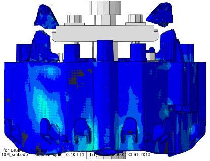
44 Example: airbag housing Source:e-Xstream

45 Impact on failure With Fiber Orientation Source:e-Xstream Isotropic

46 Choosing the right properties Properties change over product operational temperature Properties change with environmental exposure Orientation (fiber-filled plastics) Viscoelastic (time-based behavior) Creep Stress relaxation Effect of strain rate