Uncertainty Estimation in Matrix-based Life Cycle Assessment Models

Transcription

1 Uncertainty Estimation in Matrix-based Life Cycle Assessment Models Submitted in Partial fulfillment of the requirements for the degree of Doctor of Philosophy in Civil & Environmental Engineering Xiaoju Chen BS in Water Sewerage & Supply Engineering, Harbin Instituted of Technology MS in Municipal Engineering, Harbin Institute of Technology MS in Civil and Environmental Engineering, Carnegie Mellon University Carnegie Mellon University Pittsburgh, Pennsylvania April, 2017 ii

2 Copyright 2017 Xiaoju Chen All Rights Reserved iii

3 Acknowledgements This work was supported by the Pennsylvania Infrastructure Technology Alliance, the Carnegie Mellon Department of Civil and Environmental Engineering, the MaoYisheng Graduate Fellowship for the academic year, and the PNC Center for Financial Services Innovation at Carnegie Mellon University. My sincere thanks to all those who played a role in funding my degree. I want to thank H. Scott Matthews (primary advisor) and W. Mike Griffin (co-advisor) for their advice and support through my four years of study at Carnegie Mellon University. I want to give special thanks to Scott, for his understanding, patience and humor. I would not have enjoyed my work at CMU as much without his personal and research insights. I am also grateful to my other three committee members: Chris Hendrickson, Eric Williams, and Brandon Kuczenski, who provided many helpful comments on my work. I would also like to thank Daniel Posen, Lauren Cook, Ken Sears, and my other CEE and EPP friends for their research insights. Finally, I would like to give special thanks to Josue Orellana, for his help and support on preparing this dissertation. 4

4 Abstract Life Cycle Assessment (LCA) has been applied to help decision-makers understand quantitative environmental effects and impacts through the life stages of a product or process. Matrix-based LCA models are widely incorporated to LCA software tools to simplify the assessment and provide straightforward results. However, these tools do not sufficiently provide the uncertainties that arise from the inventory data as well as from the matrix-based models. To address this problem, in this thesis I use a range method to explore three types of uncertainties (parameter, scenario, and model uncertainties) present in matrix-based LCA models. These three types of uncertainties are assessed separately for two different types of LCA models: the Input-Output- based LCA model, and the process-based LCA models analyzed with matrix methods. IO-based LCA models are studied with the Environmental Input-Output Life Cycle Assessment (EIO-LCA) model, and the US LCI database incorporated to matrix methods is used as an example of process -based LCA models. I selected two demonstrate the results with two environmental effects (greenhouse gas emissions and energy consumptions) and five environmental impacts (global warming, ozone depletion, acidification, eutrophication and ecotoxicity). First, I analyzed the parameter uncertainty in the EIO-LCA model. Publicly available data sources and assumptions are used to estimate the parameter uncertainties of the direct energy consumption in the US industrial sectors. The direct and indirect energy consumption ranges are estimated through the EIO-LCA model. The results show that the parameter uncertainties are generally within -40% to 40% from the default values, with several outliers. Second, I examined the scenario uncertainties in total carbon dioxide emissions by using alternative inputs in the US LCI database. I found that the US LCI database fails to take full advantage of matrix-based methods; when incorporated to matrix-based LCA models, less than 10% of the processes contribute to the indirect environmental effects. The results of scenario uncertainty estimation in the US LCI database show that on average, the total carbon dioxide emissions across all processes are between -30% to -30%. Finally, I addressed the model uncertainty by using different Life Cycle Inventory Assessment (LCIA) methods incorporated in the matrix-based models. The results show that when the US LCI inventories are applied, the uncertainties due to choosing different impact 5

5 methods are within 5%. This is possibly caused by the incompleteness of the inventories: more than 50% of the characterized substances are excluded in the inventory, resulting in the neglect of some impact values. The results from this study emphasize the importance of estimating uncertainties in matrix-based LCA models. The variability in the LCA results is caused by all three types of uncertainties, as well as the incomplete inventories embedded in the matrix-based LCA models. Future LCA database and software should focus on including uncertainty estimation in the features and improving the inventory data to take full advantage of the matrix-based LCA models. 6

6 Table of Contents Acknowledgements... 4 Abstract... 5 Table of Contents... 7 List of Figures List of Tables Chapter 1. Introduction and Bacround Motivation Introduction Life cycle assessment Matrix-based LCA models Uncertainty in LCA Life cycle impact assessment (LCIA) Dissertation outline and research questions Chapter 2. Parameter uncertainty in the EIO-LCA model Parameter uncertainty in matrix-based tools Material and Methods Values in the R matrix Data sources Assumptions and calculations Results and discussion Uncertainty results for single sectors Uncertainties of the g vector Sectoral impact to overall model Uncertainty values re-evaluation Decision support considering uncertainty Case Study 1 Illustrating impact of uncertainty on the results Case Study 2 Identifying uncertainty related to specific fuel use

7 2.4.3 Case Study 3 Identifying hotspots given uncertainty Conclusion Chapter 3. Data analysis in the US LCI database and scenario uncertainty in matrix-based models Introduction of the matrix-based method Definitions of connections and processes Matrices mapped from unit processes in the US LCI database Cut-off processes Cradle-to-gate and gate-to-gate processes Product flows and elementary flows Connections in the US LCI database Comparisons of the interconnections between the US LCI database and the EIO-LCA model Classification based on ISIC code Number of interconnections in the IO table Classification based on ISIC code Hotspots in the EIO-LCA and comparison results Comparison with the IO table based on individual processes Scenario uncertainty estimation in the US LCI database Scenario uncertainty in US LCI processes Scenario uncertainties in US LCI industries Conclusions for the chapter Chapter. LCIA uncertainty in a process-based LCI database Introduction to LCIA and the comparison between LCIA methods Life cycle impact assessment Differences in LCIA methods Matrix-based LCA model and LCIA Inventories reporting regarding environmental impacts Summary of impact categories and substances Variability in the impact assessment results in the US LCI database

8 4.4 Validating substances coverages and variability in the impact assessment results based on individual processes Impact based inventory reporting criteria Discussion Chapter 5. Conclusions and future work Research question and answers Conclusion Future work Analyze the uncertainties of other environmental effects in the matrix-based LCA models Quantify the relationship between the technology matrix and the environmental matrix Estimate scenario uncertainty using other LCI databases Test the correlation between number of substances covered and the total impact results Improving the minimum report value criteria Appendix References

9 List of Figures Figure 2-1: Method used to calculated different B values from different R matrices that has substitutes Figure 2-2: Scaled results for 1 million dollars of final demand of sector No. 120 (Petrochemical manufacturing). Total energy as well as separated fuel consumptions are provided. Abbreviation: NG as natural gas, Petrol as petroleum products, N-F-Elec as non-fossil fuel electricity Figure 2-3: Scaled results of total energy consumption and top 15 energy intense sectors for $200k final demand of sector No. 120 (Petrochemical manufacturing). Graph on top is the g values (direct and indirect); the bottom shows the top 15 energy intense sectors for the g values Figure 2-4: Results of the B matrices for all 428 sectors, based on percentage changes comparing with default value. Linear scale is used for negative values while base 10 logarithmic scale is used for positive values Figure 2-5: Results of g values for all 428 sectors, based on percentage changes compared to default value. Linear scale is used for negative values while base 10 logarithmic scale is used for positive values Figure 2-6: Scaled results of total energy consumption for approximately 170,000 paper and plastic cups Figure 2-7: Results of energy consumption for 1 km concrete and asphalt pavement, error bars are the max/min values without outliers Figure 3-1: Definitions of upstream and downstream connections in this study, shown with one downstream connection and two upstream connections for a hypothetical Process A Figure 3-2: Number of upstream connections for each process in the US LCI database. The inset provides greater detail for those processes with 10 or less process inputs. Values on the x axis indicate the number of connections in which each process falls. For example, the third bar on the main graph shows that there are 272 processes that have a range from 6 to 10 upstream connections. Results are shown separately for Cut-off (blue), and non-cut-off processes 10

10 (orange). The bar on the zero value is the number of processes with no upstream connection. All Cut-off processes have zero upstream connections, due to the inventory unavailability Figure 3-3: number of downstream connections for each process in the US LCI database. The inset shows processes with 10 or less downstream connections. Result are shown separately for cut-off (blue) and non-cut-off processes (orange). Values on the x axis indicate the number of connections in which each process falls. For example, the third bar on the bottom graph shows that there are 19 processes that have connections ranging from 11 to 20; 9 of these processes are cut-off processes. The bar on the zero value is the number of processes with no downstream connections Figure 3-4: different types of connections among the 1471 processes in the US LCI database. The chart on the right shows the different types of connections shared by the 1471 processes, the figure on the left shows processes that have fuel (green circle), electricity (brown circle) or transportation (blue circle) as inputs, for the processes that have one or more than one upstream or downstream connections Figure 3-5: Numbers of connections for agriculture, industrial and transportation sectors (331 in total) in the IO table (service sectors not considered). The left histogram shows the numbers of downstream connections; the right histogram shows the numbers of upstream connections Figure 3-6: highlights of connections in IO table (left) and US LCI database (right). Values between the lowest and highest were highlighted in 3 color scales: white (lowest), yellow (0.01% of the highest), and red (highest). Grey area were processes in the US LCI database that have no accurate matches in the IO table, such as coal, combusted in industrial boiler process Figure 3-7: Overall scenario uncertainty caused by using direct alternative electricity inputs. The default electricity input for each process was the electricity input from the original inventory. Left: fossil CO2 emissions, as percentage difference from the default, for 876 gate-to-gate processes (without cutoff processes). Right: the emissions for each process were calculated by using 78 grid electricity and 21 fuel electricity scenarios, without the outliers caused by using Electricity, onsite boiler, hardwood mill, average, NE-NC. Each scenario used one of the 99 electricity generation processes as electricity input

11 Figure 3-8: Overall scenario uncertainty caused by using both direct and indirect alternative electricity inputs. The default electricity input for each process was the electricity input from the original inventory. Left: fossil CO2 emissions, as percentage difference from the default, for 876 gate-to-gate processes (without cutoff processes). Right: the emissions for each process were calculated by using 78 grid electricity and 21 fuel electricity scenarios, without the outliers caused by using Electricity, onsite boiler, hardwood mill, average, NE-NC. Each scenario used one of the 99 electricity generation processes as electricity input Figure 3-9: Overall scenario uncertainty caused by using alternative electricity inputs. Y-axis represents 876 gate-to-gate processes (without cutoff processes) in the US LCI database. Values on the x-axis are the ratios of total to direct fossil CO 2 emissions Figure 3-10: Fossil CO2 emissions for one metric ton of Iron, sand casted. Left: scenario uncertainty caused by using grid electricity. Right: scenario uncertainty caused by using fuel electricity. The top graphs show the total emissions. The bottom graph shows the results from the top ten product contributors under alternative scenarios (markers) Figure 3-11: Total fossil CO2 emissions for one metric ton of Iron, sand casted, considering four different cases Figure 3-12: total fossil CO2 emissions, in, for 1 ton of Benzene, at plant by using alternative scenarios in electricity and transportation industries. The default values are circled and the default inputs are listed Figure 3-13: fossil CO2 emissions, in, for 1 metric ton of Manufacture of basic iron and steel category (top), and Manufacture of basic chemicals (bottom) Figure 3-14: legend for Figure Figure 4-1: Elements of the LCIA phase provided in ISO (ISO 2006b) Figure 4-2: Numbers of Global warming (GW) substances in the gate-to-gate process from the US LCI database. The processes were sorted from the largest number of substances (left) to the smallest (right). The two values for each process are the maximum and minimum number of substances in 14 popular impact assessment methods (see Table 4-2). The cut-off processes in the US LCI database are not shown in this figure, as these processes do not have any output 12

12 component. Also omitted are the processes without GW substances after No The first 10 processes names are shown in the table Figure 4-3: Non-zero values for the US LCI processes that have the largest numbers of global warming (GW) substances. The marked cells in the tables represent non-zero values. Cells with red borders are reported as non-zero values by the EPA GHGRP. The direct and indirect tables were obtained from the B matrix, and g vector for each process respectively (the non-zero values are highlighted in orange) Figure 4-4: Non-zero values for the US LCI processes that have only one global warming (GW) substance. The highlighted cells in the tables represent non-zero values. Cells with red borders are reported as non-zero values by the EPA GHGRP. The process number corresponds to the x- axis in Figure Figure 4-5: GW values in CO2 eq perfunctional unit, from 14 impact methods, marked by the different symbols described in the legend. Processes No.1 to No.10 are shown on the left, and processes No. 11 to No. 50 are shown on the right. The processes are sorted by total impact results including direct and indirect impacts. The first 10 processes names, industrial categories, functional units, and original index numbers from the US LCI database are listed in the table. 127 Figure 4-6: GW values in CO2 eq per functional unit from 14 impact methods for processes No. 50 to No The processes are sorted from high to low by the total impact results including direct and indirect impacts. Other processes with zero GW impact from any of the methods are not shown Figure 4-7: GW impact values in CO2 eq per ton-km for 190 transportation processes in the US LCI database Figure 4-8: GW impact values in CO2 eq per kwh for 98 electricity processes in the US LCI database Figure 4-9: GW impact values in CO2 eq per for 23 plastic material processes in the US LCI database Figure 4-10: Total GW impacts for the Crude palm kernel oil, at plant process calculated from 14 different methods. Two of the 14 methods listed in the figure have different covered substances (The markers are the same as in Figure 4-5)

13 Figure 4-11: Testing the relation between the results from Global Warming and substance completeness proportions. The marker color indicates different alternative scenarios. The black line is the fit obtained from a linear weighted least squares regression

14 List of Tables Table 2-1: Energy prices used in this study Table 2-2: Summary of different data sources and assumptions used in the uncertainty range model. Default value is annotated Table 2-3: Detailed descriptions of assumptions used in data sources Table 2-4: Result from controlled tests, sectoral results (Million TJ) Table 2-5: Energy Consumption for 1km concrete pavement Table 2-6: Energy Consumption for 1km of asphalt pavement Table 3-1: Inputs in the gate-to-gate and cradle-to-gate processes for PET production from Franklin Associates original LCA study. The two processes differ in material usage and inputs.. 59 Table 3-2: Inputs in the gate-to-gate and cradle-to-gate processes for PET production provided by the US LCI database. Italics are used to mark the differences from Table 3-1. The inputs for the cradle-to-gate process are broken into upstream raw elementary flows, as opposed to the inputs as product flows from the original LCA study Table 3-3: top ten fossil CO2 emissions processes for producing 1 of Polyethylene terephthalate, resin, at plant (PET), calculated from the gate-to-gate PET process Table 3-4: process and resource elementary flows Table 3-5: Processes with more than 20 downstream connections in the US LCI database Table 3-6: Processes with more than 20 downstream connections in the US LCI database, sorted by three industrial categories Table 3-7: top 5 inputs for Cement manufacturing, sorted by direct economic values in the IO table, and mass values in the US LCI database, respectively Table 3-8: Fossil CO2 emissions to produce 1 metric ton of Portland cement, calculated from EIO- LCA model (left) and the US LCI database (right). The shaded rows show the total CO 2 emissions, including both direct and indirect emissions. The remaining rows show the top 10 emissions from different sectors or processes Table 3-9: Mean and standard deviation of the minimum or maximum values for all 876 processes, based on four different cases

15 Table 4-1: Numbers of characterized substances in major impact categories (columns) for 45 impact assessment methods (rows). The displayed methods are embedded in the SimaPro software (version 8.3). Highlighted rows with red and Italic font are the methods chosen for demonstration in this study Table 4-2: characterization factor values (in CO2 eq) for all 110 global warming (GW) substances generalized from 14 popularly used impact methods Table 4-3: Elementary flows for Mercury with different impact regions and compartments in the US LCI database Table 4-4: GW substances in the US LCI database and their characterization factors in different methods Table 4-5: Summary of the number of substances and matching elementary flows in five selected impact categories for the US LCI database Table 4-6: Mandatory Greenhouse gases reported to the US EPA GHGRP for each industry. Cell listed as EPA are emissions reported under the mandatory reporting rule. Cells highlighted with red color are emissions that are not included in any of the US LCI process within each industry Table 4-7: GW substances for the Crude palm kernel oil, at plant process, and impacts for the substances calculated from 14 impact methods. The cells with larger values are highlighted with darker bacround Table 4-8: Maximum characterization factor value and new cut-off criteria for each substance. Cut-off criteria were based on 5% and 1% of total GW for 1kWh Electricity, bituminous coal, at power plant The first 34 GW substances are shown as examples

16 1. Chapter 1. Introduction and Bacround 1.1 Motivation Life cycle assessment (LCA) is a decision-support technique for practitioners, including policy makers and industry, to assess the environmental impacts of a product or process. The results from LCA studies can aid the decision-makers by providing quantitative environmental impact results (Hellweg and Canals 2014). LCA software tools, such as OpenLCA, SimaPro, and CMLCA, have been designed for conducting LCA studies and are popularly used by environmental specialists and decision makers. These tools provide accessible LCA results and have lower barriers to be understood and handled compared to the scattered scientific LCA reports published in academic journals. However, the user-friendly interfaces of LCA tools have insufficient uncertainty information to make the users fully understand the underlying information behind the data and the results. This lack of sufficient uncertainty information limits the accuracy of decision-making based on the results provided by the LCA tools. The LCA tools often incorporate matrix-based methods in the analyses of LCA results. Due to the complexity of matrix-based methods, the uncertainty estimation in the LCA tools are hard to be addressed. The existing tools use only empirical judgments and simulations to estimate the uncertainties in the LCA tools. The estimated uncertainties from such methods are hard to interpret and can be easily ignored by the users. In order to provide the users with more reliable uncertainty results in LCA tools, more robust uncertainty estimation methods for matrix-based models need to be developed. More accurate uncertainty information for LCA tools needs to be provided. This dissertation attempts to analyze the uncertainty associated with the data inputs and model outputs of matrix-based LCA tools. A method using real-life data rather than empirical estimation based on the quality of the deterministic data is developed, and the uncertainties of matrix-based LCA tools are estimated based on the new method. In addition, the uncertainties from the empirical estimation method are applied to current available full datasets used in the inputoutput matrix-based model to compare with the uncertainty results estimated from the new method. 17

17 In this study, a new method to estimate the uncertainty in matrix-based LCA models will be provided. The method is based on more reasonable estimation and assumptions, and provides more robust uncertainty results in matrix-based LCA models. The proposed method can be easily applied to both process matrix LCA and input-output LCA models. The uncertainty results will help matrix-based LCA tool users have an insight of the importance of uncertainty in LCA models, and provide more understandable uncertainty results to support the decision-making process associated with LCA. 1.2 Introduction Life cycle assessment Life Cycle Assessment (LCA) is a method that computes and evaluates the inputs, outputs, and environmental impacts from design to disposition of a product or process (Guinee 2002; ISO 2006a). The guidelines developed by the International Organization for Standardization (ISO) regulate the minimum requirements in the principles and framework of LCA studies (ISO 2006b). Based on the ISO standards ISO and 14044, LCA studies involve four main phases: 1) the goal and scope definition that defines the context of the study, 2) the life cycle inventory (LCI) that creates an inventory of stages and flows, 3) the life cycle impact assessment (LCIA) that evaluates the environmental impacts based on the inventory, and 4) the interpretation that systematically interprets the results (ISO 2006a). Three primary types of LCA methodologies have been applied to determine environmental impacts and help in decision making: process-based LCA that analyzes the impacts from the processes involved in a study, economic input-output LCA (IO-LCA) that uses economic exchange values to trace the total impacts from the supply chain, and hybrid LCA that combines process-based and input-output-based methods to combine and expand the perspective of the two methods (Hendrickson et al. 1998) (Hertwich 2005) (Finnveden et al. 2009) (Pairotti et al. 2014). Following the four stages and conducting an LCA study in each of the three primary types is time consuming; this is a complex processes that requires data gathering, study scoping, inventory and impact estimation as well as result interpretation (Ong et al. 2001). Different LCA databases and 18

18 LCA tools have been developed to help the users perform LCA studies in more efficient and convenient ways. LCA software tools such as Gabi, SimaPro, BEES, EIO-LCA and LCA databases such as Ecoinvent and U.S. LCI use existing inventory data, and include various models and methods to quickly generate systematic results for users (GmbH 2006) (Consultants 2008) (NIST 2009) (National Renewable Energy Laboratory 2012) Matrix-based LCA models The efficiency of LCA analysis can be improved by scaling the inventory in matrix-based models. Compared to scattered scientific LCA models, matrix-lca models provide accessible results and have lower barriers to be understood and handled. The Life Cycle Inventory (LCI) data from existing LCA databases (U.S. LCI, ELCD and Ecoinvent) can be mapped on to a matrix model. Recently, the matrix-based LCA models have been widely accepted and incorporated to LCA software tools (Heijungs and Suh 2006). Matrix-based methods are applied to Input-output (IO) LCA models. IO LCA is a method that combines LCA and the economic input-output approach, which is applied in the principles of Input-output models developed by Leontief (Leontief 1970). The IO method scales the direct requirement exchanges in dollar values between industrial sectors into matrix A, and uses Leontief inverse (I A) 1 to include the upstream requirements of the sectors. The A matrix can be the regionally specified input-output table from economic surveys. For example, the 2002 Standard Use Table provided by the US BEA is used in the IO-LCA model developed at Carnegie Mellon University. IO-LCA applies the environmental effects from the industries to the Leontief inverse and estimates the total environmental effects from productions in the industries. The process-based LCA can also apply the matrix methods to scale the inventories and provide both direct and indirect effects. The principles are the same for the two different models with slight differences. First, the process-based LCA considers the exchanges between product flows, not industrial sectors. Second, in process-based LCA, the direct requirements are scaled into the A matrix based on physical units. In this way, the exchanges between processes are based on the functional units of the production, instead of dollar values as used in IO-LCA models. Third, instead of Leontief inverse (I A) 1, the inverse of the A matrix is used in estimating the total 19

19 requirements. Despite the three minor differences, the two models have the same advantage of efficiently providing both direct and indirect effects. However, both models also suffer from the lack of uncertainty information. In this study, the parameter uncertainties of these two models are accessed. I use the US 2002 Economic input-output life cycle assessment (EIO-LCA) model s energy consumption category to implement and demonstrate the utility of the uncertainty estimation method in the IO LCA model. The US LCI database are incorporated into matrices to provide the uncertainties in the process - based LCA methods Uncertainty in LCA LCA practitioners have long been trying to consider uncertainty information in LCA studies to give more robust conclusions (Huijbregts 1998; Lloyd and Ries 2007; Williams et al. 2009). Huijbregts et al. (2003) outlined three sources of uncertainty: parameter uncertainty, scenario uncertainty, and model uncertainty. Parameter uncertainty arises from using inaccurate data and weighting factors in the LCI analysis (Huijbregts 1998). Scenario uncertainty includes different choices such as scope, system boundaries, and allocation methods. Model uncertainty is caused by spatial differences as well as characterization factors. These types of uncertainties are propagated to the life cycle results via different methods, such as probabilistic (Bullard et al. 1988; Raa and Steel 1994; Ali and Santos 2014), fuzzy (Tan 2008; Cruze et al. 2012), and range analysis (Chevalier and Téno 1996; Geisler et al. 2005; Deng et al. 2011; Bawden et al. 2015). In probabilistic methods, random samples are generated by distributions that are defined to represent uncertainties in the inventory data. Each distribution is estimated or chosen based on its parameters such as mean, standard deviation, and distribution type (e.g., normal or uniform). The parameters and type of distribution can be estimated with different methods, including: applying the regression results of various data sets (Lenzen 2001; Yamakawa and Peters 2009; Lenzen et al. 2010), assumptions made for estimating the impact multipliers (Zhang, et al 2014), or by using the pedigree matrix approach (Weidema and Wesnæs 1996). The fuzzy number approach uses fuzzy logic to estimate uncertainty in the degree of plausibility of data (Tan 2008). The range method applies multiple values for each process to 20

20 represent the uncertainty. The multiple values are collected for each process and are treated equally as possible inputs in the inventory resulting in a range of possible values in the final answer. In current practice, parameter uncertainty in matrix-based LCA models has been addressed by using a pedigree matrix approach (Weidema and Wesnæs 1996). This approach determines the parameter uncertainty from the data indicator scores, which quantitatively estimate the quality of the data sources. In practice, this approach requires a considerable number of assumptions and simulations. Some LCA software tools like SimaPro, include this analysis. However, estimating parameter uncertainty in this way is problematic, in two ways. First, the uncertainty distributions from the inventory data are arbitrary. The data indicator scores and pedigree matrix approach focus on quantifying the quality of each data point s data source, rather than the quality of the data points. The distributions are not estimated from real data samples, but rather empirical judgement. Second, the uncertainty results are hard to interpret. Generally, LCA practitioners are not capable to easily understand the methodology of parameter estimation and simulation. It is hard to interpret the uncertainty in the results without knowing the causes. Scenario and model uncertainties have not yet been addressed in matrix-based LCA models. Here, the scenario uncertainty can be caused by scaling inventories with different goal and scope to the same matrix; while the model uncertainty can come from different impact assessment methods being incorporated into the software. Compared with the parameter uncertainty, the scenario and model uncertainties from matrix-based LCA models are more easily overlooked. When a matrix-based model scales inventories with different goal and scope together without any distinction, the users are unable to realize the result contains scenario uncertainty. Similarly, the model uncertainty cannot be identified unless the potential uncertainty results are given directly to the users. In current practice, LCA tools that apply matrix-based methods generally do not clearly provide potential scenario and model uncertainties to the users Life cycle impact assessment (LCIA) Life cycle impact assessment (LCIA) is a phase of life cycle assessment (LCA) (ISO 2006b). This phase seeks to evaluate the environmental impacts from a product system (Owens 1997). To 21

21 achieve this evaluation, Life cycle inventory (LCI) data are associated with environmental impact categories (ISO 2006b). Multiple impact assessment methods have been developed for different purposes of the LCA studies. Early impact assessment developments were based on the only available reference - ISO standard (Baumann and Rydberg 1994). In 1999, the SETAC-Europe working group provided guidance to impact assessment method developments, in order to model the best available impact assessment method (Udo de Haes et al. 1999). The concepts of impact assessment framework, and principles of characterization factor modeling are widely accepted and adapted in LCIA developments. Many LCIA methods have been developed since, some of which are updated regularly. These methods provide characterization factors to transform environmental effects to quantified environmental impacts. In matrix-based LCA models, to evaluate the total environmental impact results for products under study, the LCIA methods are applied to the inventories and effects. LCIA methods provide different characterization vectors to transform the effects. The differences in the characterization factors are the contributors to the model uncertainties in matrix-based LCA models. LCA studies have focused on the uncertainties in the LCIA results regarding the differences in LCIA methods. Baumann and Rydberg (1994) compared three early LCIA methods: ecological scarcity (ECO), environmental theme (ET), environmental priority strategies in product design (EPS). For these three methods, Baumann and Rydberg looked at the differences between the calculation methods for characterization factors. Pennington et al. (2004) also systematically reviewed the differences between multiple impact assessment methods regarding their models and methodologies. More recently, some LCA studies have considered the variances in the impact results caused by choosing different impact methods (Brent and Hietkamp 2003; Bovea and Gallardo 2006; Cavalett et al. 2013; Owsianiak et al. 2014; Martinez et al. 2015). All of these studies emphasized the importance of choosing the best-suit impact assessment method for the goal and scope of the study. However, no LCA study has focused on understanding the model uncertainty caused by using different LCIA methods in matrix-based LCA models. 22

22 1.3 Dissertation outline and research questions In this study, I introduce methods to comprehensively address the three types of uncertainties in matrix-based models. For reference, I have applied our methods to two different matrix-based models: the IO-LCA model, and the process-based LCA model. Following the introduction (Chapter 1), the dissertation is divided into three research chapters and a concluding chapter, followed by appendices and references. The main chapters and the research questions they explore are outlined below. In chapter 2, the parameter uncertainty in matrix-based LCA models is estimated using an IO LCA model. Key research questions include: What are the uncertainty ranges of direct and indirect life cycle energy consumptions over the supply chain of the U.S. industries based on economic input-output models with public available data? What is the impact of each individual industry s uncertainty on results of other industries? Which industries have the largest uncertainties in the model? How to reduce the uncertainties of these industries? In chapter 3, the parameter uncertainty is estimated for process -based LCA inventories incorporated into the matrix-based LCA model. Chapter 3 also introduces the scenario uncertainty in the same model. Key research questions include: In the current US LCI database, how many processes flows contribute to the indirect environmental effects when applied to matrix-based LCA models? What are the total CO 2 emissions ranges from US industrial processes by considering different scenarios from current process-based life cycle inventory databases? What are the ranges of total CO 2 emission ranges from aggregated US industrial processes calculated from current process-based life cycle inventory databases? In chapter 4, the model uncertainty is estimated based on the differences in the LCIA methods. Key research questions include: 23

23 In current LCIA methods, how many substances are covered? How many of these substances are included in elementary flows in the US LCI database? Does the US LCI database have enough flows that are characterized in impact assessment methods to build a robust inventory? For processes in current process-based LCA databases, what are the uncertainties of direct and indirect environmental impacts caused by different impact characterization factors used in LCIA? What are the contributions of different characterization factor values and coverages of substances from different methods to the LCA result? What should be the new reported value in LCI for different substances considering impact assessment results? 2. Chapter 2. Parameter uncertainty in the EIO-LCA model 2.1 Parameter uncertainty in matrix-based tools Parameter uncertainty arises from using inaccurate data and weighting factors in life cycle inventory analysis (Huijbregts 1998). The parameter uncertainties in the LCA inventories are propagated to life cycle results via different methods, such as probabilistic (Bullard et al. 1988; Raa and Steel 1994; Ali and Santos 2014), fuzzy (Tan 2008; Cruze et al. 2012), and range analysis (Chevalier and Téno 1996; Geisler et al. 2005; Deng et al. 2011; Bawden et al. 2015). In probabilistic methods, random samples are generated by distributions that are defined to represent uncertainties in the inventory data. Each distribution is estimated or chosen based on its parameters such as mean, standard deviation, and distribution type (e.g., normal or uniform). The parameters and type of distribution can be estimated with different methods, including: applying regression results of various data sets (Lenzen 2001; Yamakawa and Peters 2009; Lenzen et al. 2010), assumptions made for estimating the impact multipliers (Zhang, et al 2014), or by using the pedigree matrix approach (Weidema and Wesnæs 1996). The fuzzy number approach 24

24 uses fuzzy logic to estimate uncertainty in the degree of plausibility of data (Tan 2008). The range method applies multiple values for each process to represent the uncertainty. The multiple values are collected for each process and are treated equally as possible inputs in the inventory resulting in a range of possible values in the final answer. In this study, I introduce a method that adapts principles of the range method to propagate uncertainty in matrix-based models, as such methods are used in most LCA software tools to manage data and generate results. The focus in this study is on propagating and representing data (parameter) uncertainty, as applied to an input-output matrix based model. A range of alternative values developed based on different data sources with different assumptions are considered in the inventory. The data are derived from publicly available data sources such as government agencies, published research articles, and reports. Different assumptions are used to convert or estimate the raw data from these sources to derive values in an appropriate form for the model. Values calculated were used to estimate changes in results from the model s current deterministic values. A new way of visually presenting results is also introduced. I use the US 2002 Economic input-output life cycle assessment (EIO-LCA) model s energy consumption category to implement and demonstrate the utility of the method. The EIO-LCA model is used because it has a clear boundary, which includes all US industrial sectors (428 in total), providing consistency for comparison between sectors. Although, there are many potential impacts that could be model choosing energy consumption i s based on the on the high degree of data availability, and because it is a fundamental component to estimate other inventory categories, such as greenhouse gas emissions. In an IO-based matrix model, Equation 1 is used to estimate the environmental effects from all sectors defined in the system. In Equation 1, f is a vector of requirement defined by the users; it is the amount of direct purchase from the industry in dollar value. For an economic system that has n industries, the f vector has n by 1 dimensions. The A matrix is n by n, each column or row represents an industry in the system. The A matrix can be the regionally specified input-output table from economic surveys. For example, the 2002 Standard Use Table (the Use Table) provided by US BEA (ref) is used in the IO-LCA model developed Carnegie Mellon University (ref). The B 25

25 matrix is an m by n matrix, the rows are m different environmental effects cause by producing dollar units of product in each industry (represented by impact/$). The resultant vector g, has m by 1 dimensions and contains the m total environmental effects for the final demand f. For each environmental effect ( i = 1,, m ), the direct and indirect effects can be separated by the Hadamard (entrywise) product of the transpose of row i in the B matrix and (I A) 1 f: Equation 1: g = B(I A) 1 f Equation 2: h i = B T i (I A) 1 f This approach provides a method to quickly scale large inventory data to estimate the final impact, saving users time and effort. As the direct and indirect effects can be separated, the large indirect effects contribute to the total effects can be sorted to identify the hotspots in the upstream production. LCA tools, such as EIO-LCA, can provide the users these hotspots in the results; the hotspots are straightforward and can help to identify the important upstream industry to reduce the effects. However, LCA tools fail to emphasize uncertainty, which is critical in determining the impact of LCA results and conclusions (Wang and Work 2014). Common LCA tools typically show only deterministic results; since no uncertainty is displayed, users or the study audience may assume that there is no relevant uncertainty. The following sections describe the methods used in developing these uncertainty-based estimations in the 2002 EIO-LCA model with respect to energy consumption. The detailed information of sectors in the EIO-LCA model are provided in Table S1 in the Appendix. 2.2 Material and Methods This section explains the method used to evaluate B matrices. I also provide a description of the data sources and assumptions. Finally, the method used for propagating the uncertainty are introduced Values in the R matrix In a deterministic input-output model, an energy B matrix contains the unit energy consumption of each industry sector based on the economic exchange between industries, making the unit in 26

26 the energy B matrix Joules/$. Two steps are involved in estimating values in a B matrix: first, annual energy consumption values for each industry are estimated from available data sources; second, the energy values are normalized (divided) by the total annual economic output of the industry sector. In the new method, instead of a single deterministic value, multiple energy consumption values were derived by using various available data sources to generate an energy consumption range for each sector. Those different consumption values were estimated from different sources like survey reports, e.g., with different assumptions about fuel prices. The detailed estimations of data points are discussed below Data sources Energy consumption values were calculated from various publically available data sources. From the different data sources as well as various assumptions (see section Assumptions and Calculations), multiple values were developed for each sector. For the energy consumption category in the 2002 EIO-LCA model, data from 6 publicly available government agency sources were used: U.S. Bureau of Economic Analysis (US BEA) U.S. Census Bureau (Census) U.S. Department of Energy, Energy Information Administration (US EIA) U.S. Environmental Protection Agency (US EPA) U.S. Department of Agriculture (USDA) National Transportation Research Center (NTRC). The 2002 Standard Use Table (the Use Table), provided by US BEA, has expenditure data for the energy production sectors (in million $) for all 428 US industrial sectors. An advantage of the Use Table is the availability of sectoral level data for electricity, coal, petroleum fuels and natural gas consumption for all 428 sectors. Due to the completeness of the data, the Use Table has traditionally been used as a major data source in IO-based LCA models (including the EIO-LCA model). Values in the Use Table were converted from expenditure values to physical units with various price assumptions. 27

27 Table 2-1 shows the prices used in all the sectors when no more specific price data is available. Values are provided by U.S. Energy Information Administration (Forms EIA-782A, "Refiners'/Gas Plant Operators' Monthly Petroleum Product Sales Report" and EIA-782B, "Resellers'/Retailers' Monthly Petroleum Product Sales Report). The prices were used to convert fuel expenditure values in U.S. dollars to energy consumption values in physical units. Table 2-1: Energy prices used in this study Fuel type Value Unit Coal 1.25 $/MBtu Natural Gas 4.02 $/1,000 cu. Ft Motor Gasoline $/gal Kerosene-Type Jet Fuel $/gal Kerosene 0.99 $/gal No. 1 Distillate $/gal No. 2 Distillate $/gal No. 2 Diesel $/gal No. 2 Fuel Oil $/gal No. 4 Distillate $/gal Residual Fuel Oil $/gal The U.S. Census Bureau was another major data provider across nearly all sectors. Detailed reports including Industry Series Reports for mining, construction, and manufacturing sectors; Core Business Statistics Series; and the Business Expenses Survey were applied to evaluate energy consumption values for agriculture, mining and mineral, construction, utility, manufacturing, transportation and service industry categories. Values from the Census required conversion from North American Industry Classification System (NAICS) codes to IO codes, as well as from expenditure values to physical units with price assumptions, if the values were provided by expenditure value. Some data sources were used only for a broad industry category. For instance, two energy surveys, the US EIA s Manufacturing Energy Consumption Survey (MECS) and Commercial Buildings Energy 28

28 Consumption Survey (CBECS) were major data sources for manufacturing and service sectors. MECS provides detailed fuel and electricity usage in both physical units and expenditure dollar values. CBECS provides energy consumption and expenditure values for commercial buildings. The values are in a form of building types aggregated by principal building activities, such as education, food services and health care. These two surveys have the disadvantage that some of the values were aggregated to higher-level sectors, which required allocation in order to provide values at the 428 industrial sector level. Values from US EPA, USDA and the Transportation Energy Data Book published by National Transportation Research Center (NTRC) were used for energy estimation for utility, agriculture, and transportation sectors. The data gathered from these different data sources were processed by recalculating, allocating or aggregating with assumptions. A full report of how the data were processed can be found at (Chen et al. 2016) Assumptions and calculations Applying the range method, different values were calculated to form alternative B matrices, rather than using one deterministic B matrix to estimate a deterministic g vector. These B matrices were calculated from different data sources with different calculation assumptions. The methods vary across sectors, but generally include price assumptions for unit conversion, allocation for aggregated values in raw data, and missing raw data evaluation. Energy consumption values from different data sources were not necessarily in physical energy units. For instance, expenditure values were commonly provided, as in the Use Table. In these cases, data were converted to physical units of energy with fuel prices. As price values were not always available for individual sectors, sectors were grouped into categories where one of its members energy price was known. For instance, CBECS provided fuel prices based on building types, the price values for the building type education was assigned to three sectors: education services, social assistance, and national security & international affairs. This a ssignment was based on the definition of the building type education from CBECS (US EIA 2003). 29

29 Allocation was required when the energy data was at an aggregate level compared to that needed for the EIO-LCA model. These values were allocated into their sub-sectors using allocation factors that were situation dependent. For example, while MECS provided energy consumption values for manufacturing sectors, they were often at the 3-digit NAICS code level rather than the 6-digit level needed for the model. In these cases, fuel expenditures in dollars from the detailed Use Table were used as allocation factors to estimate the 6-digit sectoral fuel consumption. The assumption presumes that sectors within an aggregate industry sector have similar costs of energy. Fuel use values were allocated from the 3-digit to 6-digit sector level by considering the dollar purchases of the fuels of each commodity sector in the model from the relevant industry. For example, in the Food sector (3-digit NAICS code 311), if sector (6-digit NAICS code) represented 90% of purchases from the Coal mining sector for all the sectors beginning with 311, then 90% of the coal use would be allocated to sector Some data sources provide reports with partially withheld data, in these cases, missing data were estimated using different methods, such as adapting data from previous years. In the US Census Industry Series Reports for mining, the physical units of energy consumption for a few sectors were withheld. Two general methods were used to estimate the missing values: 1) deriving missing values based on logical deductions; 2) the energy expenditure ratio of the sector to the total mining category. The uncertainties in the B matrix are then propagated through the model to calculate the life cycle final results. The direct and indirect (total) consumption is the value in the g vector, calculated by Equation 1. Instead of using only one B matrix, I used various B matrices to estimate different g vectors; those B vectors were used to form the ranges. Besides the default matrix, which was chosen as a set of values falling in the middle of all the available data sources, 30

30 and is generally the current EIO-LCA deterministic results with a few exceptions 1, alternate B matrices were formed using data from one data source and calculated with the one assumptions. This enables investigators to make different assumptions to select the B matrix values that meet the purpose of their analyses. Presenting results calculated from same data source/assumptions can more clearly present the overall uncertainty for users, and avoid weighting methods. Table 2-2 and Table 2-3 show the summary of different assumptions and data sources used in each alternative B matrix (USDA 2002a; Census 2007a; MECS 2002; NTRC 2014; EIA 2004). A brief description of data sources and assumptions used to convert values are listed below; a more detailed document can be found at (Chen et al. 2016). USDA: United States Department of Agriculture (USDA) 2002 Census of Agriculture provided the expense of total gasoline, fuel and oil (but not electricity) in dollar values for agriculture sectors in its report (USDA 2002b). Prices in Table S1 are used to convert the energy expenditure values to physical units. Use Table 1: the US 2002 Standard Use Table (the Use Table) provided by Bureau of Economic Analysis (BEA 2002) has the detailed expenditure values from other sectors to one sector (in million dollars). In the Table, the purchases from Coal mining, Power generation, Natural gas distribution, and Petroleum refinery sectors for all other remaining sectors are used as the energy purchase values. Prices in Table S1 are used to convert the energy expenditure values to physical units. Use Table 2: values in the Use Table are used as the energy purchase values. Different prices are used to estimate energy consumption values. The prices are provided by the 2002 Manufacturing Energy Consumption Survey (MECS 2002), and the Commercial 1 A default value in the analysis represents the base case of the percentage change. The default value for each sector was chosen as a set of values falling in the middle of all the available data sources. In most of the cases, the default value is the value used in the current EIO-LCA model. In two cases, default values in this study are not equal to those in the current EIO-LCA model: 1) values that are updated with new evaluated withheld data, a few manufacturing and mining sectors have these updated values; and 2) values that calculated based on more specific price assumptions, these values are used in natural gas and gasoline product consumption for service sectors. 31

31 Buildings Energy Consumption Survey (CBECS 2003). MECS provides the unit prices of different fuel types in its reports: Average Prices of Purchased Energy Sources 2002, with the unit dollar per physical unit and dollar per million BTU. CBECS provides fuel expense values and energy consumption values based on the types of the building, these values are used to calculate the unit price of the fuels regarding individual building types. These less aggregated unit price values are used to convert the energy expenditure values to physical units. US Census mining 1,2,3,4,5: US Census of Bureaus 2002 Economic Census Industry Serious Reports (2007) provided fuel and electricity usage in physical units (e.g., short ton, barrel, cubic feet, gallon and kwh) as well as economic expenditures in some cases for the mineral sectors in Two different allocation methods are used for the withheld data points in the source. Method 1 was used in estimating current values in EIO-LCA mode; method 2 involves some new assumptions and re-evaluation. Two major differences are: 1) various fuel prices were used, rather than fixed fuel price; 2) withheld data were re-estimated in order to better fix the total fuel expenditure values provided by Census Mining Report. US Census construction 1,2: US Census of Bureau s reports Construction: Subject Series - Industry General Summary: Detailed Statistics for Establishments by Subsector: 2002 and Construction: Industry Series: Detailed Statistics for Establishments: 2002 are used to estimate the energy consumption values for construction sectors. The two reports provide energy consumption values in four different categories: Gasoline and Diesel, Natural gas, Electricity, and Other fuels in dollar value; Prices in Table S1 are used to convert the energy expenditure values to physical units. In addition, the values in the reports are provided by NAICS code, a bridge developed by Sharrard (2007) was used to convert the NAICS code to IO code: each NAICS construction industry was allocated into one or more different IO industries based on a mathematical method. CBECS 1,2: the Commercial Buildings Energy Consumption Survey (CBECS 2003) conducted by US Energy Information Administration (US EIA) is used for energy consumption values, allocation is needed. The values provided by CBECS are in both energy consumption value in physical units and expenditure value in dollars. The values are based on the types of the 32

32 building, such as education, rather than industrial codes. Therefore, values from CBECS are allocated into different sectors based on the crosswalk between CBECS buildings and NAICS industries. In this file, different types of building activities were allocated to its likely corresponding NAICS sectors. For example, the building type category education was considered to be most likely allocated into 611 Education services, as well as two other sectors 624 Social assistance and 928 National security and international affairs. Then the NAICS sectors were converted to IO based sectors. MECS 1,2,3: 2002 Manufacturing Energy Consumption Survey (MECS 2002) provides energy consumption values for manufacturing sectors. The survey also provided standard errors for the values. These values are all used in the scenario ranges. Data provided by MECS are in physical units, but generally aggregated at the 3-digit NAICS level, values were allocated from the 3-digit to 6-digit sector level by considering the dollar purchases of the fuels of each commodity sector in the model from the relevant industry sectors. EPA: Data from National Greenhouse Gas Emissions Data (Table A Energy Consumption Data and CO 2 emissions from Fossil Fuel Combustion by Fuel Type ) reported by EPA (2014) were used as coal, natural gas and petrol consumptions for Power generation sector. These values are provided in physical units, merely for electricity generation; no further calculation and conversion are needed. NTRC: Transportation Energy Data Book (2014) conducted by Oak Ridge National Laboratory and published by the U.S. Department of Energy. Its 24 th edition reported the consumption of energy in physical units by fuel type and transportation mode for the year The energy consumption values are used for the transportation sectors. Figure 2-1 tries to more visually describe the substitution process used (as first mentioned in the paper) for when a data source does not cover all 428 sectors. Three different substitutes are used to replace the missing values. For example, if one data source (US Census) only provides data for sectors No. 20 to 30, the rest of 418 sectors need substitutes in the R matrix. Three different cases of choosing three different substitutes will result in three different B values: asterisk, plus, and circle symbol shows the result of using default values, minimum values, and maximum values for each sector as substitute, respectively. 33

33 Figure 2-1: Method used to calculated different B values from different R matrices that has substitutes In the cases where partial data were available, such as B matrix No. 3 in Table 2-2, All the results are chosen as they could be helpful to understand possible outcomes caused by different assumptions. 34

34 Table 2-2: Summary of different data sources and assumptions used in the uncertainty range model. Default value is annotated. Default Sector categories B matrices Agriculture Manu- Mining Utility Construction facturing USDA d Census EPA d Construction MECS1 d US US Census Mining 1 d 1 Use Table 1 2 Use Table 2 US Census 3 Mining 2 US Census 4 Mining 3 US Census 5 USDA d Mining 4 EPA d US Census 6 Mining d US Census MECS1 d Construction 1 d MECS US Census MECS 3 Mining 1 d US Census MECS1 d Construction 10 2 d default value used as substitute Transportation NTRC d NTRC d Service CBECS 1 d CBECS 1 d CBECS 2 CBECS 1 d The values used in the B matrices are not necessarily independent. Results could be from the same data source, but with different assumptions. Two alternative B matrices are both calculated from the Use Table, with different price assumptions. The same energy purchase values are used for each sector, only the fuel price (divisor) for each sector changes; therefore the energy consumption results are highly interdependent. Also, some raw data used in the data sources 35

35 were derived from common economic surveys. The values for mining sectors, construction, and agriculture sectors were all derived from the US Economic Census, meaning that the data sources are not entirely independent. All the results are chosen as they could be helpful to understand possible outcomes caused by different assumptions. 36

36 Table 2-3: Detailed descriptions of assumptions used in data sources Abbreviation Calculation description Calculation methods Use Table 1 Use Table 2 US Census Mining 1 US Census Mining 2 US Census Mining 3 US Census Mining 4 US Census Mining 5 MECS 1 Fix fuel prices provided by EIA are applied to convert values for all sectors Different fuel prices to convert individual sectors, the prices values are gathered from different data sources, such as CBECS and MECS Withheld fuel expenditure are estimated based on the sum of rows and columns, different fuel prices (from Census Mining) are used to convert values for each sector Withheld fuel expenditure are estimated based on the sum of rows and columns, fixed fuel prices are used to convert values for each sector Withheld fuel expenditure are estimated based on the ratios from total, different fuel prices (estimated for individual sector from Census Mining) are used to convert values for each sector Withheld fuel expenditure are estimated based on the ratios from total, fixed fuel prices (estimated for all sectors in the category from Census Mining) are used to convert values for each sector Withheld fuel expenditure are estimated based on the ratios from total, fixed fuel prices (from EIA) are used to convert values for each sector Default values provided by MECS are used, some values are calculated based on allocation, expenditure values from the Use Table are used as allocation factor Price assumptions for unit conversion Price assumptions for unit conversion Missing raw data evaluation, price assumptions for unit conversation Missing raw data evaluation, price assumptions for unit conversation Missing raw data evaluation, price assumptions for unit conversation Missing raw data evaluation, price assumptions for unit conversation Missing data evaluation, price assumptions Allocation for aggregated values in raw data 37

37 MECS 2 MECS 3 CBECS 1 CBECS 2 USDA EPA NTRC Minimum values provided by MECS are used, some values are calculated based on allocation, expenditure values from the Use Table are used as allocation factor Maximum values provided by MECS are used, some values are calculated based on allocation, expenditure values from the Use Table are used as allocation factor Some values are calculated based on allocation, 'converting bridge' provided by CBECS is used allocation factor; different fuel prices to convert individual sectors, the prices values are gathered from different data sources, such as CBECS and MECS Some values are calculated based on allocation, 'converting bridge' provided by CBECS is used allocation factor; fixed fuel prices to convert individual sectors, the prices values are gathered from different data sources, such as CBECS and MECS Some values are calculated based on allocation, expenditure values from the Use Table are used as allocation factor; fix fuel prices provided by EIA are applied to convert values for all sectors Some values are calculated based on allocation, values from the same data source are used as allocation factor Some values are calculated based on allocation, expenditure values from the Use Table are used as allocation factor Allocation for aggregated values in raw data Allocation for aggregated values in raw data Allocation for aggregated values in raw data, price assumptions for unit conversation Allocation for aggregated values in raw data, price assumptions for unit conversation Allocation for aggregated values in raw data, price assumptions for unit conversation Allocation for aggregated values in raw data, price assumptions for unit conversation Allocation for aggregated values in raw data 38

38 2.3 Results and discussion This section shows how the method is implemented in the 2002 EIO-LCA model, using IO Sector No. 120, Petrochemical manufacturing, as an example. Additionally, three case studies are used to demonstrate the potential improvement in decision support considering the uncertainties and results Uncertainty results for single sectors Figure 2-2 shows the results for total energy consumption across the supply chain as well as separated by fuel for IO Sector No. 120, Petrochemical manufacturing. The names in the legend indicate different alternative B matrices used to estimate the result (Table 2-2). All the results are chosen as they could be helpful to understand possible outcomes caused by different assumptions.. Three other B matrices that use each sector s minimum/maximum/default value generalized from all alternative results are also provided. The results are based on one million dollars of final demand input in sector 120. Since IO-LCA models are linear, the relative uncertainty for a different input of final demand would be the same. In this case, the sector s total energy consumption varies from 21 TJ to 62 TJ, resulting in the range of -50% to 40% compared to the default value of 42 TJ. Figure 2-2 shows that the uncertainties of natural gas and petroleum usage are the major contributors to the large discrepancy of total energy consumption. They are also estimated to be the highest fuel inputs in the total. The causes of the uncertainties are also displayed in Figure 2-2. The red symbols are the values calculated from the B matrix using values from the Use Table. All of the red symbols are larger than the value calculated from the default B matrix, which demonstrates that the values in the Use Table tend to be the upper values within the ranges. In addition, the uncertainty in the total energy consumption is mostly caused by the large uncertainty of petroleum consumption associated with data from the Use Table, of which possible reasons are discussed later in this paper. The results calculated from the US Census data (blue symbols in Figure 2-2) are closer to the default value. Since only a small proportion of data come from the Census, and a majority of the data are substitutes, the results are similar to the results calculated from default values. 39

39 Figure 2-2: Scaled results for 1 million dollars of final demand of sector No. 120 (Petrochemical manufacturing). Total energy as well as separated fuel consumptions are provided. Abbreviation: NG as natural gas, Petrol as petroleum products, N-F-Elec as non-fossil fuel electricity. As a hotspot analysis tool, IO models like EIO-LCA can deterministically list the highest sectors across the supply chain for an industry. Figure 2-3 shows the results of the top 15 most energy intense sectors in the supply chain for 200 thousand dollars of final demand in sector 120, sorted by the values in the deterministic B matrix used in current EIO-LCA model. As can be seen, sector 120 (Petrochemical manufacturing), 115 (Petroleum refineries) and 126 (Other basic organic chemical manufacturing) are the top 3 energy intense sectors, contributing an estimated 64% to the total energy consumption. These three sectors are also major contributors to the uncertainty of total energy consumption; however, the rankings of the top 5 energy intense sectors could change when uncertainties are considered. The red symbols for the top 3 sectors remind us that the Use Table is the data source leading to the high end of the ranges. As these sectors belong to the Petroleum Product Manufacturing category, this finding indicates that the Use Table provides greater energy consumption values for some petroleum products. Similar conclusions can be 40

40 made for values from CBECS, which provides relatively smaller values for petroleum products. The reason for these differences is discussed in the following section. Figure 2-3: Scaled results of total energy consumption and top 15 energy intense sectors for $200k final demand of sector No. 120 (Petrochemical manufacturing). Graph on top is the g values (direct and indirect); the bottom shows the top 15 energy intense sectors for the g values. 41

41 Figure 2-4: Results of the B matrices for all 428 sectors, based on percentage changes comparing with default value. Linear scale is used for negative values while base 10 logarithmic scale is used for positive values. 42

42 Figure 2-5: Results of g values for all 428 sectors, based on percentage changes compared to default value. Linear scale is used for negative values while base 10 logarithmic scale is used for positive values. While Figure 2-3 suggests sectors with high default values also have high uncertainty for Sector 120, this is not a general rule - uncertainty varies across many dimensions. Figure 2-4 shows the uncertainty results of all 428 sectors in all B matrices, based on each sector s percentage change, compared to its default value. Note that the positive side of the x-axis is transformed to log scale for legibility. Results suggest that in general, the sectoral uncertainty for direct and indirect energy consumption in the B matrix is approximately ±50% overall. In some extreme cases, the values reach over 40 times larger than the default value. For example, the value for Coal mining (No. 21, noted by the dashed arrow in Figure 2-5) varies from 5 to 70 TJ/M$, and Petroleum lubricating oil and grease manufacturing (No. 118, noted by the solid arrow in Figure 2-5) varies from 3 to 110 TJ/M$. Such outcomes demonstrate how different data sources and assumptions can result in a significantly larger range for some sectors, which would not be currently expressed in such models, like EIO-LCA. Results from Figure 2-4 also show that Use Table (red) and MECS (green) generally 43

43 lead to values larger than the default while US census of construction (purple) generally lead to lower values. This analysis suggests that the uncertainty in the energy B matrix can be large. Thus using only a single data source for a sector in the B matrix (as typically done in IO-LCA models) could ignore important information about the system Uncertainties of the g vector Figure 2-5 shows the results of the g values, which include the total of direct and indirect energy consumption calculated from Equation 1 for $1 million final demand for each industry, based on different B matrices. Detailed percentage changes for all 428 sectors are shown in Table S1 of the Appendix. The results were calculated based on the total economic output in 2002 for each sector. The overall uncertainty in total energy consumption for a sector varies from about -40% to 40%; however, for several extreme cases, the result is approximately 5 times larger than the default value. The percentage changes are smaller compared to changes in the B matrix, especially for the extreme cases, given the interconnectedness of supply chains. The results show that the percentage changes in the g vector are generally less than the changes in the B matrix, based on the composition of the overall supply chain. The different patterns of uncertainties are caused by the discrepancies in the values of the g vector, which are taken from various data sources. Using this information, potential sectors with large uncertainties could be identified or adjusted after further investigation, in order to reduce the uncertainty in the model. The next section briefly discusses how to investigate the reasons for large discrepancies, by re-evaluating data sources Sectoral impact to overall model In matrix-based LCA models, the change of one sector s value in B matrix can have impacts on the whole model. In order to show the impacts from single sector to the overall model, controlled tests are conducted and compared with base case results. The controlled tests are performed by setting the value of one of the 428 sectors in B matrix as upper or lower bound while holding all 44

44 other 427 sectors constant at their default values, and the results are compared with base case, which uses default value for each sector. A top ten detailed sectoral results is shown in Table 2-4. Not surprisingly, Power generation has the most impact to the model; and considering both sides from the default value, Pipeline transportation is another very important sector cause the total changes is 3 million TJ. These sectors, though have relatively smaller uncertainties, have the largest impacts on the model. The controlled test of the study provides information of the importance of the sectors to the model. The importance of the sector does not depend on the energy intensity or the uncertainty of the sector, but the relations of each sector to the rest 427 sectors in the model. Hospital sector has a total 2 million TJ energy consumption value and more than 500% upper uncertainty results, however it has negligible impacts over other sectors as well as the model On one hand, this information will benefit the decision makers by providing supporting information of selecting the most sensible sectors, user will be able to choose the best suitable information to reduce the uncertainty in their LCA analysis. Values provided in Table 2-4 show both the changes of each sector and the changes of the rest of the sectors caused by the sector. For a sector such as hospital that has big sectoral change but small impact over the rest sectors, the uncertainty is only important when this sector s result is investigated in a LCA study. On the contrary, coal mining sector, which has both big sectoral change and big impact over the model, needs to be taken serious account anytime. On the other hand, as matrix-based LCA model involves a great amount of calculation, the information will help the user to decide with sectors should be taken into more serious account to limit the calculation time in matrix-based LCA models. So far the high uncertainty flows have not been addressed in uncertainty analys es in matrix-based LCA models. The results in this study will support further uncertainty estimation and sensitivity analysis in matrix-based LCA models. 45

45 I-O number Table 2-4: Result from controlled tests, sectoral results (Million TJ) Sector name Change without sectoral change (real) Change with sectoral change Sectoral change Change Default value to Power generation and supply Min Petroleum refineries Max Oil and gas extraction Min Iron and steel mills Max Coal mining Max Other basic organic chemical manufacturing Max Pipeline transportation Max Pipeline transportation Min Petroleum lubricating oil and grease manufacturing Max Asphalt paving mixture and block manufacturing Max Other basic organic chemical manufacturing Min The analyses above are based on the exchanges between sectors within the boundary set by the IO table (the entire production of the economy), thus the results are limited to the energy consumption within the system boundary set for a certain year and geographic area. For example, several studies suggested that energy embedded in infrastructure should be included in the supply chain of a process (Chester and Horvath 2009; Lucas et al. 2012; Turconi et al. 2013). However, this part of the energy is not within the system boundary of the EIO-LCA model. Several industrial sectors such as Nonresidential manufacturing structures are included in the IO table; however, the exchange between other sectors and these construction sectors are based on the 46

46 year 2002, excluding energy embedded in the infrastructure already built. Therefore, the results in Table 2-4 are limited to the system boundary of the EIO-LCA model; if the users need to include processes outside the boundary, the results might change depending on the boundary drawn for the new analysis Uncertainty values re-evaluation The existence of major discrepancies for some of the sectors is one of the novel results presented. Tracking the reasons for these can provide decision makers with a clearer concept of how or when to use the various data given the uncertainties. An example is shown in Figure 2-3. Larger than default values were calculated from the Use Table (red), while smaller than default values were calculated from CBECS (light blue). A possible explanation is the insufficient documentation of the data source. Values provided by the Use Table were based on the purchase of all fuels for the sector, rather than energy consumed specifically in production phases. For example, these purchases could include fuels used as both energy and feedstocks. The resulting uncertainty can be reduced as better-documented data are provided (I note that MECS separates fuel and feedstock usage but is more aggregated than values in the Use Table). An extreme example of data induced uncertainty can be found in the Coal mining sector. The minimum value of coal consumption for the Coal mining sector was calculated from the Census, while the maximum value was from the Use Table. Comparing the Use Table with other data sources, it was found that coal purchases between coal companies included coal undergoing beneficiation, which was accounted as an energy source purchase in the Use Table. The values generated from these data sources, including those not well-documented, were used in the analysis. As all the data sources are government agency surveys or peer-reviewed published articles, the possible reason for the differences among sources could not always be confirmed. With all the data sources separately noted in the result, users can make decisions based on all the information provided. For example, a data source for a particular sector may be excluded by the user, changing that range accordingly. An example of the utility and impact of data exclusion can be seen in case study 2. 47

47 2.4 Decision support considering uncertainty The results propagated from the uncertainties in the inventory in the EIO-LCA model can improve the utility of this source of information. As shown below, adding representations of uncertainty enables two-dimensional hotspot screening tools. The first dimension relates to the most important effects, and the second is their relative uncertainty. Either or both can indicate where additional data (e.g., primary data or sector-specific data) could be useful in subsequent efforts. Three case studies are shown that demonstrate how the information from our results can be used. All are based on previously published LCA work; I update the studies using the 2002 EIO-LCA model and present results with consideration of uncertainty. These case studies demonstrate that with such uncertainty results, 1) the LCA conclusions can be strengthened; 2) the uncertainty source can be identified; and 3) hotspots can change Case Study 1 Illustrating impact of uncertainty on the results LCA was at the center of the paper vs. plastic debate of the early 1990s (Hocking 1991). In a previous study, Lave and colleagues compared the toxic releases and energy use (electricity only) of plastic and paper cups using a 1987 EIO-LCA model (Lave et al. 1995). They estimated that 170,000 plastic cups consumed almost 50% less electricity (4,400 kwh vs. 8,600 kwh) than paper cups. The Paperboard container manufacturing and Plastics material and resin manufacturing sectors were chosen to represent paper and plastic cups respectively; total energy rather than only electricity was evaluated. The deterministic results using the models default values show that total energy consumption for 170,000 paper cups and plastic cups are 0.4 and 0.5 TJ, respectively, suggesting that plastic cups consume more energy than paper cups, different than previously stated perhaps due to exclusion of fuels. Adding uncertainty, total energy consumption for a plastic cup and a paper cup varies from 0.25 TJ to 0.69 TJ, and from 0.28 TJ to 0.45 TJ, respectively, as shown in Figure 2-6. The results with the consideration of uncertainty suggest that plastic cups use energy at the same level or higher than the paper cup production. The plastic cup has a larger range of possible energy use values than the paper cup. When results are compared on a data source by data source basis, the plastic cup 48

48 always consumes more energy than the paper cup, except for the minimum value. These results suggest strongly that beyond the previous simple deterministic results, it is very likely that plastic uses more energy, e.g., when all individual (mostly independent) data sources suggest higher values for a plastic cup, the comparison between two types of cup is more robust. Figure 2-6: Scaled results of total energy consumption for approximately 170,000 paper and plastic cups Case Study 2 Identifying uncertainty related to specific fuel use Similar to case study 1, all the assumptions except for the price values from the old study are adapted to the new study. In Horvath and Hendrickson s study (1998), the concrete pavement is made of 78,066 steel bars and 720 square meters of concrete, while the asphalt pavement takes 5,018 MT of asphalt. In this study, new price assumptions are used. U.S. Department of Transportation s report Price Trends for Federal-Aid Highway Construction provides the material prices for highway constructions from 1972 to 2006 (USDOT 2002). According to the data, prices of steel, concrete and asphalt were $0.61/lb, $25.86/sq.yd., and $34.14/ton in Therefore, the expenditures of one kilometer-long cement concrete and asphalt pavement are $0.13 million ($106,000 steel and $22,270 concrete) and $0.19 million. Applying these expenditure values to EIO-LCA model, Iron and steel mills, Ready-mix concrete manufacturing, Asphalt paving mixture and block 49

49 manufacturing sectors are used for three components, energy consumption results for two types of pavements are shown in Table 2-5 and Table 2-6, respectively. Table 2-5: Energy Consumption for 1km concrete pavement Fuel types Upper Lower Min (GJ) Default (GJ) Max (GJ) uncertainty (%) uncertainty (%) Coal % -68% Natural gas % -28% Petroleum products % -100% Non-fossil electricity % -32% Biomass % -3% Total % -54% Table 2-6: Energy Consumption for 1km of asphalt pavement Fuel types Min (GJ) Upper Lower Default Max (GJ) uncertainty uncertainty (GJ) (%) (%) Coal % -40% Natural gas % -28% Petroleum products % -100% Non-fossil electricity % -15% Biomass % -3% Total % -46% Updating to the 2002 EIO-LCA model and using the Iron and steel mills, Ready-mix concrete manufacturing, and Asphalt paving mixture and block manufacturing sectors to represent the pavement products, it was found that the deterministic total energy consumption for 1 km of asphalt and concrete pavement changed to 4 TJ and 5 TJ, respectively, favoring the choice of asphalt on an energy basis. As the analysis based on EIO-LCA model relies on the prices of the products, the differences from the prior analysis are possibly due to the significant change of the prices of asphalt and concrete over 10 years. However, the results remain deterministic, 50

50 encouraging users to make assertive decisions; the question becomes whether considering uncertainty in the model can better assist the LCA analyses. Figure 2-7: Results of energy consumption for 1 km concrete and asphalt pavement, error bars are the max/min values without outliers As shown in Figure 2-7, considering all values, the energy consumption for 1 km of asphalt pavement has a range from 1.9 TJ to 17.8 TJ, larger than that of concrete pavement (2.3 TJ to 6.2 TJ). Asphalt pavement could be nearly 8 times (17.8/2.3) more energy intense, in contrast to the conclusion based on simple deterministic values. The large range in total energy use for asphalt pavement is mostly associated with the uncertainty of petroleum usage. As mentioned previously, the Use Table indicates larger petroleum purchase values for petroleum product manufacturing industries due to potential feedstock use. The uncertainty could be reduced if improved documentation was available. Providing all the results can allow users to make decisions based on all available data. The users can choose to ignore the big outliers caused by insufficiently documented data. For instance, if the values from the Use Table are ignored, the ranges for asphalt pavement change to 1.9 TJ to 3.7 TJ, resulting in a maximum value for asphalt pavement smaller than the maximum value for concrete pavement. 51

51 2.4.3 Case Study 3 Identifying hotspots given uncertainty LCA models, specifically IO-LCA models, are often used as a hotspot screening tool to help decision-makers access quick and simple relative results. The importance of sectors regarding environmental impact rankings helps determine what and where to look for potential impacts in a supply chain. Ukidwe and Bakshi (2008) developed a model to evaluate the environmental impacts of the chemical industry. In one step of the analysis, an economic input-output (EIO) model was used to identify the most significant supplier in an industry s supply chain. EIO models provide the economic outputs for all sectors in the supply chain; the most significant supplier can be found by sorting the outputs. Ukidwe and Bakshi identified that the most important supplier is the Petroleum refineries sector regarding economic output for the Petrochemical manufacturing sector. Inspired by Ukidwe and Bakshi s study, I use the 2002 EIO-LCA model to evaluate the energy consumption for Petrochemical manufacturing. In our analysis, rather than economic output, energy consumption is evaluated and shows that the most energy intense sector is Petrochemical manufacturing. When considering uncertainty, the most significant supplier can change. As shown in Figure 2-3 (which is the relevant result to use for this case study), when all possible data points are considered, Petrochemical manufacturing, Petroleum refineries, or Other basic organic chemical manufacturing could be the most energy intensive sector in the supply chain. If uncertainties are not considered, the possibility of the other two sectors being the most significant supplier may be ignored, and they could be left out of the analysis or not be a focus of study. 2.5 Conclusion This study develops a method that propagates and visualizes uncertainty, focusing on inventory data uncertainty, in matrix-based LCA models. The uncertainty results provide additional insight to understand how a screening tool framework can be used to identify both the importance and the uncertainty of the results. Considering the uncertainty can provide better decision support for LCA studies, leading to more robust decisions as compared to those using only deterministic values. Different data sources and assumptions were used to build different underlying matrices 52

52 of direct and indirect energy consumption values for each sector. The different consumption values provide information that can be used to identify the source of the uncertainties. A benefit of this approach is that it can be extended easily as additional relevant data sources are identified. Results show that uncertainty in the B matrix in the EIO-LCA model is generally around 50%, with some extreme cases that reach over 40 times the default value. The overall uncertainty of each sector considering both direct and indirect impacts is smaller; total energy consumption, considering all 428 industries, is generally within -40% to 40%, with a few extreme cases that have over 4 times more impact. Outliers show that even reliable data sources can lead to large uncertainty, especially when underlying assumptions are not well documented or understood. Another contribution of this paper is the visualization of all possible values calculated for one sector. The results visually show all possible results calculated from different data sources and/or assumptions, rather than merely the maximum and minimum values for a sector. There are several advantages of this visualization. First, results emphasize all possible results, which cannot be indicated in simple bounding results. Second, more information can be provided when possible results are shown to users. Users can make judgments based on all the information shown in the visualization. Third, users can track the source(s) of uncertainty in the inventories by reading the possible results. The general method used here for energy consumption can be applied to other inventory categories of an IO-LCA model, can be expanded to consider scenario and model uncertainties. The method described here can be used to inform an uncertainly analysis in process matrix models as well and could consist of known ranges of values for a sub-process input into the B matrix or simply deriving a range of data from the various complementary available process datasets. As an example, if electricity is important in the process and the model has various data to represent electricity generation (grid average, renewable, fossil fuel-based, etc.), a range can be generated to help an analyst to explore and present the impacts. Future work will focus on adapting the method to the uncertainty estimation in the technology and intervention matrices of process-based models. 53

53 3. Chapter 3. Data analysis in the US LCI database and scenario uncertainty in matrix-based models 3.1 Introduction of the matrix-based method Process-based data is typically used in LCA, and when implemented in software using existing databases, is often modeled with matrix-based methods. The method scales life cycle inventories from existing databases into matrices, and uses formulas (such as Equation 1) to calculate the direct and indirect environmental effects for any user-defined final demand in the system (Heijungs et al. 1992; Heijungs 2010; Heijungs and Suh 2006; Wang and Work 2014). The results calculated from the matrix-based LCA method can separately provide environmental effects of direct (onsite) and indirect (upstream) processes in the system under study. The system under study may consist of all processes provided in a LCA database. These databases, such as US LCI (United States Life Cycle Inventory) and Ecoinvent, often provide LCI data for a significant amount of processes. The LCI data generally includes direct (gate-to-gate) energy, materials used, and emissions from the production of the processes (NREL et al. 2004). To assess the direct environmental effects from production, the LCI of each process can be used individually. The LCI data of different processes can also be grouped together using matrix-based methods to include both direct and indirect environmental effects. A brief description of how inventories are mapped into matrices is provided below. The inputs and outputs in a unit process from a LCA database are one of two types: product flows or elementary flows. The product flow is an input or output from the technosphere (technical system or the economy) (NREL et al. 2004). Electricity generated from coal is an example of a product flow. An elementary flow is an environmental effect to the biosphere (nature or ecosystem) without previous human transformation (ISO 2006b) (NREL et al. 2004). Carbon dioxide emitted to air is an example of an elementary flow. In process-based LCI databases, each unit process has its product flow mapped on to the technology matrix (A), and its elementary flow mapped on to the intervention matrix (B). These two matrices are used in Equation 3 (Heijungs 2010) to calculate direct and indirect environmental effects. 54

54 Equation 3: g = BA 1 f Where f is a vector representing the final demand defined by the users; it is the amount of product output in its functional unit. For a system that has n unit processes and m elementary flows, the f vector has n by 1 dimensions. The A matrix is n by n, each column represents a unit process and each row indicates the input/output product flow. The B matrix is an m by n matrix, here the rows are m different elementary flows, such as carbon dioxide emissions. A 1 f gives an n by 1 vector of the total input/output product flows. The resultant vector g, has m by 1 dimensions and contains the m total environmental effects for the final demand f. For each environmental effect ( i = 1,, m ), the direct and indirect effects can be separated by the Hadamard (entrywise) product of the transpose of row i in the B matrix and A 1 f: Equation 4: h i = B T i A 1 f Where h i is an n by 1 vector containing the i th environmental effect from n unit processes for the final demand f. 3.2 Definitions of connections and processes Two directed connection categories among processes are defined: downstream and upstream (Figure 3-1). The downstream connections of a process indicate the relative role of the process in the database. An electric power generation process, for example, was typically used as an energy input in industrial productions, thus many downstream connections would be expected. Figure 3-1 shows the downstream and upstream connections for a hypothetical process A. On the right panel, two input product flows are related to Process A via upstream connections (Process B and C). The left panel shows the definition of a downstream connection. When a process serves as an input to another process, I say that the input process has a downstream connection to the receiving process. Process A has one downstream connection, to Process B, which of course then has an upstream connection to Process A. As shown in this example, an upstream connection could be another process downstream connection, or vice versa. 55

55 Figure 3-1: Definitions of upstream and downstream connections in this study, shown with one downstream connection and two upstream connections for a hypothetical Process A. As the LCI for each process only provides direct inputs or outputs, the indirect inputs or outputs calculated from the matrix-based LCA method rely on the interconnections between processes in the system under study. These interconnections are links between processes based on their respective inventories. In the matrices, a link between two processes is represented by a nonzero value. In recent years, the interconnections in the LCI database have become interesting to LCA practitioners. Using graphical methods, Kuczenski (2015) estimated the interconnections between processes in several LCI databases; this study concluded that all the databases under consideration shared similar internal structure. Network analysis methods have also been used in input-output models to determine the key processes in the system (Singh and Bakshi 2011; Kagawa et al. 2013; Nuss et al. 2016). These studies generally focused on determining the strongly connected processes in the system with the purpose of categorizing processes in the databases, and identifying important processes in particular industries. However, the question of how the database interconnections affect the results from matrix-based LCA method remains unanswered. Substantial connections are crucial to evaluate direct and indirect environmental effects. The coverage of connections determines whether the indirect environmental effects can be fully captured. This study demonstrates a method to evaluate the effects from the interconnections in matrix-based methods. The US LCI database is used as a case study. The latest version of the US LCI database provides 1060 unit processes. These unit processes have inputs or outputs from 1466 elementary flows and other processes. In this study, first, the processes from the US LCI database were mapped on to the A and B matrices. Then, the inputs and outputs for each process were evaluated and quantified to demonstrate the coverages of connections in the database. Last, I compared the connections with the input-output 56 table and the results from EIO-LCA

56 (Environmental Input-Output Life Cycle Assessment) model to identify possible missing connections for some processes. In addition, I analyzed the uncertainties resulting from using alternative utilities for each process. 3.3 Matrices mapped from unit processes in the US LCI database At the time this analysis was conducted, the US LCI database provided 701 unit processes. The inventories of these unit processes could be obtained individually from the US LCI website compiled by the National Renewable Energy Laboratory (NREL 2012). To apply the inventories into matrix-based LCA model, I downloaded the inventory data for all available unit processes and used Matlab software to map their inventories into the A and B matrices (code is provided in the Appendix). Following the terminology from above, the results from the mapping showed n=1471 product flows and m=2701 elementary flows in the matrices. I observed some potentially problematic processes in the matrix mapping and results. These problematic processes affect the consistency of the inventories in the matrices and could result in inaccurate interpretations in the matrix-based LCA model. Therefore, before the interconnections in the matrices were evaluated, I screened potential problematic processes according to three categories: the cut-off processes, the system boundary, and the flow types Cut-off processes In US LCI, cut-off processes, previously labeled as Dummy processes, are input products whose inventories are not yet provided in the current version of the database. For example, the inventory information of one secondary steel production process ( CUTOFF Steel, secondary, at plant ) is not yet included in the database. Currently, 525 or 35% of the total number of processes in US LCI database are cut-off processes. The cut-off processes cover diverse products and generally can be found in all US industries, see Table S3 for a list of all cut-off processes. When the database is applied to a matrix-based LCA model, the presence of cut-off processes, as inputs to a process under study, results in the neglect of upstream effects. This is because the cut-off processes do not contribute to the indirect effects. 57

57 3.1.2 Cradle-to-gate and gate-to-gate processes Based on the inclusiveness of the processes system boundaries, data in the US LCI database is associated with two different types of unit processes: gate-to-gate and cradle-to-gate. Gateto-gate processes are unit processes for the production only; the word gate indicates the entry or exit threshold of a factory. Whereas the cradle-to-gate processes also include upstream inputs and outputs; the word cradle indicates the origin of a product. The US LCI database has around 10% cradle-to-gate processes among the total number of unit processes provided; the identification of these processes are introduced later in this section. Here, Polyethylene terephthalate (PET) is used as an example product to illustrate how the two types of processes are listed in the US LCI database. The cradle-to-gate and gate-to-gate inventories for producing PET were provided in a LCA study (Franklin Associates 2010), and are shown in Table 3-1. For PET, the cradle-to-gate process and gate-to-gate process differ in their material usage and transportation inputs. The four material inputs for the gate-to-gate process are products from other factories that are incorporated to the production of PET. The cradle-to-gate PET process is composed of crude oil, natural gas, and oxygen; these are the raw production materials for the four inputs in the gate-to-gate process. There are transportation inputs in the cradle-to-gate process, because compared to the gate-to-gate process, there are more product exchanges between factories or industrial sites. In the US LCI database, the published inventories in Table 3-1 were modified to produce two different unit processes, as shown in Table

58 Table 3-1: Inputs in the gate-to-gate and cradle-to-gate processes for PET production from Franklin Associates original LCA study. The two processes differ in material usage and inputs. Gate-to-gate PET inventory, for 1000 PET, provided by Franklin Associates study Cradle-to-gate PET inventory, for 1000 PET, provided by Franklin Associates study Material Material Paraxylene 521 Crude oil 568 Ethylene glycol 322 Natural gas 215 Acetic acid 37.2 Oxygen 223 Methanol 35.2 Water consumption cubic meter Energy use Energy use Electricity (grid) 558 kwh Electricity (grid) 882 kwh Electricity (cogeneration) 9.59 cubic meter Electricity (cogeneration) 12.1 m3 Natural gas 98.1 cubic meter Natural gas 352 m3 Bit./Sbit. Coal 18.9 Bit./Sbit. Coal 35.9 Distillate oil 12.8 liter Distillate oil 13.8 liter Residual oil 26.8 liter Residual oil 80.1 liter 59

59 Transportation Combination truck Rail Barge Ocean freighter Pipeline-natural gas Pipeline-petroleum 28.5 tkm 1633 tkm 139 tkm 2717 tkm 382 tkm 395 tkm Table 3-2: Inputs in the gate-to-gate and cradle-to-gate processes for PET production provided by the US LCI database. Italics are used to mark the differences from Table 3-1. The inputs for the cradle-togate process are broken into upstream raw elementary flows, as opposed to the inputs as product flows from the original LCA study. Gate-to-gate PET inventory, for 1000 PET, provided by the US LCI database Cradle-to-gate PET inventory, for 1000 PET, provided by the US LCI database Material Material Paraxylene, at plant 521 Coal, lignite, in ground 25.3 CUTOFF Ethylene glycol, at plant 322 Coal, unprocessed bituminous, in 326 Acetic acid, at plant 37.2 ground 222 Methanol, at plant 35.2 Gas, natural, in ground 587 Oil, crude, in ground 243 Oxygen, in air 6.46 g Uranium oxide, 332 GJ per, in ore Water, process, unspecified natural origin/m m3 Water, process, unspecified natural origin/m m3 60

60 Energy use Energy use Electricity, at grid, US, kwh Gas, natural, in ground 504 m3 Electricity, at cogen, for natural gas 9.59 m3 Oil, crude, in ground 151 turbine 98.1 m3 Energy, from biomass 5.37 MJ Natural gas, combusted in industrial boiler 18.9 Energy, from hydro power 24.8 MJ Bituminous coal, combusted in 12.8 liter Energy, geothermal 13 MJ industrial boiler 26.8 liter Energy, kinetic (in wind), converted 12.9 MJ Diesel, combusted in industrial Energy, solar MJ equipment Residual fuel oil, combusted in industrial boiler Energy, unspecified 17.4 MJ Transportation Transportation Transport, barge, diesel powered Transport, barge, residual fuel oil tkm powered 2.18 tkm Transport, pipeline, natural gas Transport, train, diesel powered tkm 1610 tkm Disposal Disposal CUTOFF Disposal, solid waste, 0.31 CUTOFF Disposal, solid waste, 128 unspecified, to municipal incineration unspecified, to municipal incineration CUTOFF Disposal, solid waste, unspecified, to sanitary landfill 4.19 CUTOFF Disposal, solid waste, unspecified, to sanitary landfill

61 CUTOFF Disposal, solid waste, unspecified, to waste-to-energy 0.59 CUTOFF Disposal, solid waste, unspecified, to waste-to-energy CUTOFF Disposal, solid waste, process, to municipal incineration As shown in Table 3-2, the gate-to-gate process provided by the US LCI database links to four other processes flows ( Paraxylene, at plant, CUTOFF Ethylene glycol, at plant, Acetic acid, at plant, and Methanol, at plant ) in the model as inputs, and the inputs are identical to the inventory provided in the original LCA study (Table 3-1). On the other hand, cradle-to-gate processes in the US LCI database (Table 3-2) link to other elementary flows as inputs, and do not have product flows. The US LCI database (Table 3-2) also includes further decompositions, derived from Table 3-1, of the inputs raw materials represented as only elementary flows. For example, Electricity (grid) is decomposed into upstream inputs such as energy from solar, and energy from geothermal. This decomposition requires additional assumptions on electricity generation methods; however, the assumptions used are not stated in the metadata of the process (or any other cradle-to-gate process in the database), making the interpretation impossible for any user. It can only be assumed that the grid electricity used in the production is a mix of electricity generated from different types of power plants. The power plants themselves use different energy sources, such as solar power, to generate electricity. Thus, in this example, the resulting cradle-to-gate PET inventory is a mix of raw energy inputs. In general, this type of decomposition allows the cradle-to-gate process to have only elementary flows as inputs. When mapping processes on to matrices, a representation of only elementary flows avoids double-counting. Double-counting occurs when matrix A includes upstream inputs; the double-count of inputs propagates to A 1 f in Equation 3. On the contrary, without double-counting, the results calculated from A 1 f correspond to only one unit of the process under study and the cradle-togate emissions in the B matrix represent the total emissions. The effects calculated from gate-togate processes can be separated into direct and indirect effects in each upstream input using Equation 4. In this way, I can trace the locations of the upstream effects. The CTG decomposition 62

62 prevents the double-counting issue. However, the necessary assumptions as well as the decomposition methods are not documented in the US LCI database. As a result, the users are unable to fully interpret the cradle-to-gate inventory. The cradle-to-gate processes and gate-to-gate processes have different system boundaries. The two types of processes should be separated when mapped into matrices to avoid potential scenario uncertainty in matrix-based LCA models. Hence, in this analysis I distinguish the cradleto-gate processes from the unit processes in the US LCI database. To categorize cradle-to-gate and gate-to-gate processes, I consider each process metadata. The metadata information includes system boundary, location, and other notes of the LCA studies. First, the cradle-to-gate processes were identified by parse matching keywords Cradle-to-gate, cradle to gate and CTG in the metadata via MATLAB software (code available in the Appendix). Then, the identified processes full descriptions were individually assessed to avoid errors in parse matching. Last, the processes with all elementary flows but no product flows as inputs were separately identified; these processes could be cradle-to-gate processes whose inventories have been simulated into elementary flows. Keyword matching identified 125 potential cradle-to-gate processes in the original LCA study (Table 3-1). This database investigated the inventories for several different plastic resins. Individual assessments revealed 61 false positives; the cradle-to-gate misclassification was due to errors in the metadata, see Table S2. From the correctly classified 64 cradle-to-gate processes, 10 processes only had cradle-to-gate inputs in part of their inventories. For instance, the Soy-based resin, at plant process was listed as part cradle-to-gate, part unit process in its metadata. Despite the lack of clarity in these inventories, I assumed it is reasonable to consider all 64 processes as cradle-to-gate. In the A matrix mapped from all US LCI processes, I observed elementary flows as sole inputs in the remaining processes. By individual assessment I found that 6 were actually cradle-to-gate processes. Four of these six misclassifications were identified as having simulated upstream energy inputs, such as PET, CTG process in Table 3-2. I assumed that gate-to-gate processes did not have to break inputs into upstream raw materials. These processes were: Corn steep liquor, 63

63 Forest residue, processed and loaded, at landing system, Wood fuel, unspecified, and Zinc, Special High Grade. The other two misclassifications were Polylactide Biopolymer Resin, at plant and Zinc, sheet ; they had other simulated upstream inputs. The final classification count was 70 cradle-to-gate processes (approximately 4% of the total). Furthermore, 48 out of the 70 cradleto-gate processes had simulated upstream inputs in the form of raw materials, such as the PET, CTG process in Table 3-2, meaning the remaining 22 processes could cause double-counting when applied to matrix-based models. The cradle-to-gate processes can provide total environmental effects without needing to use the matrix-based method, making them seemingly more convenient to use than the gate-to-gate processes. However, a disadvantage of the cradle-to-gate processes is that they fail to provide effects on different stages of the production. For example, the cradle-to-gate PET process provided in Table 3-2 indicates that the total (direct and indirect) fossil CO 2 emissions, for producing 1 of PET, is I cannot know the amount of fossil CO 2 emissions from different inputs of the production (and thus cannot evaluate sources of differences if there were alternative production processes). In comparison, by running the gate-to-gate PET process in the matrix-based model, I calculate the direct and indirect emissions from the upstream processes (the upstream processes with the highest 10 emissions are listed in Table 3-3). Gate-to-gate processes can take the full advantage of the matrix-based method by separately listing the emissions from different stages. For the PET example, the users can tell that the onsite fossil CO 2 emissions (excluding emissions from burning fossil fuel) was 72.4, only 6% of the total emissions, while the most intensive emissions were from burning fossil fuel in the production or upstream energy use. As seen in this example, gate-to-gate processes allow the LCA practitioners to efficiently interpret the LCA results. On the contrary, cradle-to-gate processes fail to deliver an equivalent breakdown of results. Another limitation of the undocumented cradle-to-gate processes is that when applied to the matrix-based method, it is impossible to improve the inventory by reducing the uncertainty in each input. For the PET example, the total fossil CO 2 emissions from the cradle-to-gate and gateto-gate differ by 1.242, with the cradle-to-gate process (not surprisingly) having a larger emission value. As the emissions by inputs from the cradle-to-gate process are not available, it is 64

64 impossible to identify what produced these discrepancies. Alternatively, in the case of gate-togate processes, improving the data quality for an input also improves the uncertainty in the total emission. For example, the largest part of fossil CO 2 emissions for producing PET is from burning natural gas in the production, therefore when this input is switched to another fuel, or the data quality of emissions from the natural gas combustion is improved, the total fossil CO 2 emissions can be updated accordingly. This update could not be possible for cradle-to-gate processes, because their emission sources cannot be tracked. Table 3-3: top ten fossil CO 2 emissions processes for producing 1 of Polyethylene terephthalate, resin, at plant (PET), calculated from the gate-to-gate PET process. Process name 65 Fossil CO 2 emissions (g) Parentage of the total Natural gas, combusted in industrial boiler % Residual fuel oil, combusted in industrial boiler % Electricity, natural gas, at power plant % Bituminous coal, combusted in industrial boiler % Polyethylene terephthalate, resin, at plant % Electricity, bituminous coal, at power plant % Transport, ocean freighter, residual fuel oil powered % Diesel, combusted in industrial equipment % Transport, train, diesel powered % Methanol, at plant % Other % Total 1, % Product flows and elementary flows As mentioned before, a gate-to-gate process should include all the possible inputs within the technosphere. This would maximize the interconnections and include all possible indirect effects. For example, when mapping the inventory from a coal power plant on the US LCI database, one should make sure that all the associated intermediate processes have been included. For example, Coal power plants use coal as their energy input, thus a product flow that represents coal combusted for energy should be chosen as one of the inputs. Choosing coal as a raw material

65 as an input would result in ignoring potentially large emissions from the coal mining process. Note that some cradle-to-gate processes in the US LCI database have already included all inputs in the elementary flows, thus the cradle-to-gate processes do not have the same problem. In this study, all 474 raw material input elementary flows were used to identify the processes that had skipped intermediate product flows. First, I distinguished the processes with any of these raw material flows as an input. Then, the distinguished processes were individually evaluated to identify the processes that had used these raw material elementary flows directly without the intermediate process. The results show that among all 1471 processes, 136 had at least one of these raw material elementary flows as inputs. After evaluating these 136 processes individually, it was found that 131 processes were either cradle-to-gate processes (54) or correctly connected to the biosphere gate-to-gate processes (77). The 54 cradle-to-gate processes had the raw material elementary flows listed in Table 3-4 as inputs due to a separate issue discussed above. The remaining 77 gateto-gate processes were correctly connected to the biosphere. For example, the Coal, in ground (hard, 30.7 MJ per ) elementary flow is an input to Anthracite coal, at mine. The Anthracite coal, at mine process is a product (product flow) which is directly produced using coal in ground as raw material. Thus, no intermediate flow was skipped. In conclusion, there are only 5 processes that possibly skipped the intermediate processes (Table 3-4). Table 3-4: process and resource elementary flows Elementary flow as inputs, Value for 1 functional Functional Product flow skipping intermediate unit (positive as inputs, unit processes negative as outputs) Winter wheat straw, production, average, 1 Energy, from biomass 15.0 MJ US, 2022 Corn stover, production, average, 1 Energy, from biomass 15.4 MJ US,

66 Switchgrass, production, US, 2022 Portland cement, at plant Iron, sand casted 1 Energy, from biomass 15.3 MJ Clay, unspecified g Gypsum g Iron ore g 1 Limestone g Raw material, unspecified g Sand, unspecified g Shale g Slate g Coal, bituminous, 24.8 MJ 1 per g Limestone g Sand, unspecified g Skipping intermediate processes can result in neglecting the upstream environmental effects. The processes fail to reach the utmost connections for the matrix-based LCA studies. Hence there is a need to resolve the inconsistencies in flow types in order to improve the database. The next section will discuss additional connection issues found in the US LCI database. 3.4 Connections in the US LCI database To understand the processes and whether they can take full advantage of matrix-based LCA models, the connections between processes were analyzed using the definition of upstream and downstream connections introduced in section 3.2. The results show that 791 out of 1471 product flows have no upstream connections; this number includes 525 cut-off processes (Figure 3-2). The absence of upstream connections neglects potential indirect effects, as discussed previously. Similarly, 503 out of the 1471 product flows had no downstream connections (Figure 3-3). The lack of upstream connections in cut-off processes is due to inventory unavailability, not zero inputs. The matrix-based models (and databases) are less useful when the inventories include cutoff processes; when the cut-off processes are replaced by other processes with full inventories, 67

67 they will have non-zero upstream connections. It is important to be aware of cut-off processes because they are used as inputs in other processes inventories (but again, have no upstream inventory). Figure 3-3 shows that almost all cut-off processes have more than one downstream connection; in fact, 28 of them have more than 10 downstream connections meaning 10 processes would otherwise benefit from them having real inventories. These cutoff processes may hide total environmental effects. Therefore, when new inventory data are incorporated in the US LCI database, the cut-off processes inventories, especially the ones with large number of downstream connections, should be prioritized to maximize the utility and completeness of the database, and avoid potentially missing total environmental effects. The results also show that global average (upstream and downstream for all processes) was 4 connections. In general, processes had more downstream connections than upstream connections; 69 processes had more than 20 downstream connections, one process ( Transport, train, diesel powered ) had 250 downstream connections. In comparison, no process had more than 51 upstream connections. Individual processes did not necessarily have more downstream than upstream connections. 68

68 Figure 3-2: Number of upstream connections for each process in the US LCI database. The inset provides greater detail for those processes with 10 or less process inputs. Values on the x axis indicate the number of connections in which each process falls. For example, the third bar on the main graph shows that there are 272 processes that have a range from 6 to 10 upstream connections. Results are shown separately for Cut-off (blue), and non-cut-off processes (orange). The bar on the zero value is the number of processes with no upstream connection. All Cut-off processes have zero upstream connections, due to the inventory unavailability. 69

69 Figure 3-3: number of downstream connections for each process in the US LCI database. The inset shows processes with 10 or less downstream connections. Result are shown separately for cut-off (blue) and non-cut-off processes (orange). Values on the x axis indicate the number of connections in which each process falls. For example, the third bar on the bottom graph shows that there are 19 processes that have connections ranging from 11 to 20; 9 of these processes are cut-off processes. The bar on the zero value is the number of processes with no downstream connections. Table 3-5 lists the non-cutoff processes with more than 20 downstream connections. Many of these processes represent very similar alternative processes, often with minor differences. For example, Electricity, at grid, US, 2000 (No. 15 in Table 3-5) and Electricity, at grid, US, 2008 (No. 11) each represent an overall US average grid mix of electricity. Here, these input processes differ only by the year. If there are multiple versions for a given type of electricity process, only one should be chosen as the input. Table 3-4 includes the numbers of downstream connections for some similar processes, such as the two electricity 70

70 examples discussed above. To understand the downstream connections from each type of input process, the connections of these similar processes were aggregated, the processes are listed by their categories in Table 3-6. The results show that energy or transportation accounted for the majority of processes with large numbers of downstream connections. These processes are similar and are often used as inputs by other processes. When one of these processes is used as an input, it is possible to consider other similar processes as alternatives. Including these possible alternatives can potentially improve the inventories and the LCA results. This is the subject of the second topic in this chapter. The upstream connections can be subdivided into three individual types based on the characteristics of their inputs: 1) cutoff or non-cutoff inputs, 2) within or without the same industrial category based on the ISIC (The International Standard Industrial Classification of All Economic Activities) code, and 3) whether energy or transportation is included. Cut-off inputs to a process, in the first type, were distinguished because they do not contribute to the indirect effects. The ISIC code used in the second type is a classification structure based on industrial economic activities (UN 2008). I chose to use the ISIC code to categorize the processes because it associates industrial products with economic activities, and its categories are more detailed than the input-output industrial sectors. In the ISIC code, the industries are categorized in broad structures called divisions; these broad structures are further separated into detailed structures called classes. The inputs arising from outside the same category were identified to show whether the processes were connected to other industries, as processes that only have inputs from the same industry could be merely the mix of similar processes. For example, the grid electricity process in the US LCI database is a mix of different electricity processes generated by different types of fuels. For the processes that had at least one downstream or upstream connection, their inputs were evaluated separately to identify whether they were fuel, electricity, and/or transportation. It can be assumed that the production of most products needs certain types of energy and transportation as inputs, therefore the processes without any energy and transportation input should be identified. I note that this is another inconsistency in the inventories of LCI databases. For example, some processes include transportation in their scope, while others do not. However, the users are generally unaware of this inconsistency and might 71

71 use a process that does not align with their scope assumptions. The proper identification of this inconsistency can lead to improvements on the processes inventories. Table 3-5: Processes with more than 20 downstream connections in the US LCI database. Number of No. Process name downstream connections 1 Transport, train, diesel powered Transport, pipeline, unspecified petroleum products Transport, barge, average fuel mix Natural gas, combusted in industrial boiler Transport, ocean freighter, average fuel mix Diesel, at refinery Transport, combination truck, diesel powered Transport, combination truck, average fuel mix 93 9 Diesel, combusted in industrial equipment Gasoline, combusted in equipment Electricity, at grid, US, Electricity, residual fuel oil, at power plant Liquefied petroleum gas, combusted in industrial boiler Gasoline, at refinery Electricity, at grid, US, Diesel, combusted in industrial boiler Electricity, at grid, Eastern US, Residual fuel oil, combusted in industrial boiler Transport, pipeline, natural gas Natural gas, combusted in industrial equipment Transport, barge, diesel powered Electricity, at grid, Western US, Quicklime, at plant 25 72

72 24 Bituminous coal, combusted in industrial boiler Transport, barge, residual fuel oil powered 23 Table 3-6: Processes with more than 20 downstream connections in the US LCI database, sorted by three industrial categories Category Process name Number of downstream connections Electricity, at grid 192 Natural gas, combusted 160 Fossil fuel and electricity as energy Diesel, combusted 89 Gasoline, combusted 83 Liquefied petroleum gas, 63 combusted Residual fuel oil, combusted 42 Bituminous coal, combusted 24 Transport, train 249 Transportation Transport, pipeline 222 Transport, barge 225 Transport, combination truck 195 Transport, ocean freighter 129 Materials Diesel, at refinery 128 Gasoline, at refinery 55 Quicklime, at plant 25 Figure 3-4 shows the different types of connections for the 1471 processes in the database. Also included in Figure 3-4 is the analysis of energy and transportation inputs for the processes that have at least one upstream or downstream connection. The results show that 342 ( ) processes (23% of the total) have at least one upstream or downstream connection. 248 (342-94) out of these 342 processes have either transportation or fuel as input. If transportation is considered as an important input to decide whether a given process inventory is fully 73

73 established, there are 76 (61+9+6) processes (5% of the total) that have both energy and transportation as inputs. On the other hand, more than 50% of the total processes have no upstream connections; this percentage includes the cut-off processes. I also note that more than 34% of the total processes do not have downstream connections. The results also show that 165 processes in the database have neither upstream nor downstream connections. Most of these processes were by-products from the production of other products, thus their inputs were not considered. For example, Steam, at uncoated freesheet mill is a byproduct of uncoated freesheet. For this production, I assumed that allocation was not necessary. Thus, the number of inputs for this by-product was zero; consequently, the number of upstream connections was also zero. Additionally, this by-product was not used as an input in any other processes inventories, resulting in zero downstream connections. Figure 3-4: different types of connections among the 1471 processes in the US LCI database. The chart on the right shows the different types of connections shared by the 1471 processes, the figure on the left shows processes that have fuel (green circle), electricity (brown circle) or transportation (blue circle) as inputs, for the processes that have one or more than one upstream or downstream connections. 74

74 Let us define a useful process as one that effectively contributes to the indirect values in the matrix-based LCA model. A useful process requires 1) at least one upstream and downstream connection, and 2) at least one energy (fuel or electricity) and at least on transportation as input. This definition is made for several reasons. First, most processes without upstream connections neglect indirect effects in the matrix-based LCA model. Second, processes without downstream connections can be seen as only a product, rather than a contributor in the database (previous studies have defined these processes as foreground processes (UNEP 2011)). Processes without downstream connections are just modeled products from the matrix; these processes do not contribute to the indirect effects for other processes when incorporated in the matrices, therefore they do not affect the results of any other process in the database. Third, processes without energy or transportation as inputs are assumed to have missed these two inputs in the inventory; in this case, it is quite possible to neglect both direct and indirect upstream environmental effects. I found only 76 useful processes in the current version of the US LCI database. It is assumed that compared to the rest of the processes, the useful processes can cover more indirect effects in the matrix-based LCA method. I believe that the processes that are not useful processes, especially the processes without upstream connections or no energy/transportation input should not be included in the matrix. The processes without upstream connections do not contribute to the indirect environmental effects when used in the matrix-based model framework, and the lack of interconnections may mislead users to assume that there are no upstream effects. Similarly, a process without energy inputs is problematic. In the production of a process, it is unlikely that no energy is used, thus, missing energy inputs in the inventory ignores the upstream effects from energy consumption. In addition, transportation can be defined to be inside or outside of the system boundary of a process. In a database, the system boundaries for all processes should be consistent to avoid ignoring neglects of effects from transportation. However, in the US LCI database, some processes have transportation as inputs while others do not; the exclusion of transportation inputs results in missing upstream effects. The missing of energy inputs and inconsistency in transportation inputs are problematic when the processes are 75

75 incorporated into a matrix-based framework. It is difficult (sometimes impossible) for users to realize when upstream effects are missing. On the other hand, when updating the database, priority should be given to the processes that have downstream connections without upstream connections, such as some cut-off processes. For these processes, if the inventories are updated, more upstream effects can be included when modeling processes that connect to them. To maximize the connections, processes with no energy inputs should be prioritized for updates. I suggest that to gather the most indirect environmental effects, the processes in the US LCI database should be updated and maintained with a matrix-based LCA framework in mind. Identifying potential missing inventories can be helpful to the inventory updates. I use an input-output table as a reference to spot locations of the potential missing inventories and identify neglected connections in the US LCI database. In the next section, I introduce methods and results for the comparison between the IO model and the US LCI database. 3.5 Comparisons of the interconnections between the US LCI database and the EIO-LCA model The technology matrix (A) in the current US LCI database is structured by mapping the physical inventory data from all processes; the processes are comprised of a wide range of industries in the US. It is ordered alphabetically. However, the analyses above show that there are processes without upstream or downstream connections, which suggests a lack of interconnections in the technosphere. To better understand the interconnections in the database, the 2002 US inputoutput table (IO table) is used as a reference to identify potentially missed connections in the US LCI database. The interconnections in the (A) matrix from the US LCI database were compared with the interconnections in the IO table; both represent exchanges in the technosphere. The interconnections in the US LCI database were then referenced with the hotspots of exchanges between industries identified in the IO table. In the IO table, the exchanges between sectors are based on direct requirements in dollar values. In this way, all purchases between industries can be translated into product exchanges. These exchanges can be good references for interconnections. In the US LCI database, the exchanges in the technosphere are based on 76

76 individual products or processes in physical unit operations. In the IO table, the exchanges are based on industry sectors with purchase values in dollars. Because the industrial categories classified by the ISIC are more comparable with the industrial sectors in the IO table, categorized the processes in the US LCI database were categorized into industrial divisions via the ISIC code. The categorization was based on the descriptions of industries provided by the ISIC code documentation and the industrial categories of the processes in the US LCI database. The industry-classified US LCI processes were aggregated and fitted into a new technology matrix that have the same format with the IO table to make a more feasibly comparison Classification based on ISIC code The International Standard Industrial Classification of All Economic Activities (ISIC) is a classification structure based on industrial economic activities (UN 2008). The industries are categorized in broad structures called divisions; the broad structures are further separated into detailed structures called classes. I categorized the processes in the US LCI database into different categories that are comparable with IO sectors. Then, the inventories of the processes were mapped to a smaller matrix that was comparable with the IO table by aggregation. The inventories for processes were aggregated to inventories for industries using the following two steps. First, for a process, the inputs from the same categorized ISIC industrial class were summed to represent the input from the industrial class. For example, the inputs of all types of electricity, such as coal and natural gas electricity, were summed to a total electricity consumption (one single number of the electricity input). Second, within each industrial class, a process was chosen to represent the industry. For instance, the Iron, sand cast process was chosen to represent the Iron and steel manufacturing industry. As the choice of a representative process can be arbitrary, this section uses the maximum input values across all processes as the values in the new inventory. The aggregated upstream inputs were mapped into a new matrix with equal rows and columns corresponding to the number of industrial classes. The industry on each row represented an industry that provided input; each column had the chosen process inventory and represented the inventory for that industry. 77

77 The 1471 processes in the US LCI database fell into 83 categories, including 76 ISIC classes and 7 fuel combustion categories. The 7 fuel combustion categories were separately listed as they represent different stages of the energy inputs. One fuel combustion category is Natural gas, combusted in industrial boiler. The corresponding upstream fuel input in this case was Natural gas, at extraction site. The process names and ISIC categories are listed in Table S3. When categorized by the ISIC code, the IO table has 136 equivalent industries, including 54 service and government sectors. Again, the service and government sectors were not included in the analysis because they were not present in the US LCI database. From the remaining 82 industries, 6 did not have equivalent correspondences in the US LCI database. Thus, only 76 industries from the IO table were compared with their corresponding aggregated US LCI industrial categories Number of interconnections in the IO table Let us first consider the number of connections from the detailed level industries in the IO table; this should provide a general idea of how different the connections are at this detailed level. I used the same method provided in section 3.4 Connections in the US LCI databaseto evaluate the number of upstream and downstream connections of the sectors in the IO table. In the detailed level IO table, there are 428 industrial sectors; 97 of these are service and government sectors that are not part of the US LCI database. I focus on the remaining 331 agricultural, industrial, and transportation sectors, because these categories are also present in the US LCI database, and thus their connections can be compared. Results show that the average number of connections in the IO table is 277 for both upstream and downstream connections. I note that connection values less than $50,000 were not provided in the table (rounded down to $0), thus the actual number of the connections could be larger. Figure 3-5 shows the histograms of downstream and upstream connections for the 331 sectors. Most of the sectors had more than 250 upstream connections, no sector had less than 150 upstream connections in the IO table. On the other hand, 57 ( ) sectors had less than 200 downstream connections, among which 5 had zero downstream connections (hunting, and construction sectors). 78

78 Figure 3-5: Numbers of connections for agriculture, industrial and transportation sectors (331 in total) in the IO table (service sectors not considered). The left histogram shows the numbers of downstream connections; the right histogram shows the numbers of upstream connections. While the IO table benefits from aggregation of sectors, the results indicate that the IO table differs from the US LCI database in number and pattern of connections. The number of connections in the IO table are significantly larger (277 on average) than the connections in the US LCI database (4 on average). The average number of connections in the US LCI database is significantly smaller despite its larger total number of processes. The IO table also differs on the pattern of connections. For instance, the majority of the sectors had upstream inputs, and only a few sectors were not used as inputs to other sectors. The number of processes with downstream connections in the IO table was higher than the number of processes with upstream connections in the US LCI database. This indicates that unlike the processes in the US LCI database, the IO table includes mostly foreground sectors (products but not contributors) Classification based on ISIC code The International Standard Industrial Classification of All Economic Activities (ISIC) is a classification structure based on industrial economic activities (UN 2008). The industries are categorized in broad structures called divisions; the broad structures are further separated into detailed structures called classes. 79

79 I categorized the processes in the US LCI database into different categories that are comparable with IO sectors. Then, the inventories of the processes were mapped to a smaller matrix that was comparable with the IO table by aggregation. The inventories for processes were aggregated to inventories for industries using the following two steps. First, for a process, the inputs from the same categorized ISIC industrial class were summed to represent the input from the industrial class. For example, the inputs of all types of electricity, such as coal and natural gas electricity, were summed to a total electricity consumption (one single number of the electricity input). Second, within each industrial class, a process was chosen to represent the industry. For instance, the Iron, sand cast process was chosen to represent the Iron and steel manufacturing industry. As the choice of a representative process can be arbitrary, this section uses the maximum input values across all processes as the values in the new inventory. The aggregated upstream inputs were mapped into a new matrix with equal rows and columns corresponding to the number of industrial classes. The industry on each row represented an industry that provided input; each column had the chosen process inventory and represented the inventory for that industry. The 1471 processes in the US LCI database fell into 83 categories, including 76 ISIC classes and 7 fuel combustion categories. The 7 fuel combustion categories were separately listed as they represent different stages of the energy inputs. One fuel combustion category is Natural gas, combusted in industrial boiler. The corresponding upstream fuel input in this case was Natural gas, at extraction site. The process names and ISIC categories are listed in Table S3. When categorized by the ISIC code, the IO table has 136 equivalent industries, including 54 service and government sectors. Again, the service and government sectors were not included in the analysis because they were not present in the US LCI database. From the remaining 82 industries, 6 did not have equivalent correspondences in the US LCI database. Thus, only 76 industries from the IO table were compared with their corresponding aggregated US LCI industrial categories Hotspots in the EIO-LCA and comparison results In this section, the connections in the US LCI database and the IO table are compared on the aggregated level of the matrices. 80

80 Figure 3-6 provides an overall comparison, using connection hotspots, between the IO table (left) and the technology matrix in the US LCI database (right). Both tables represent the A matrix in the matrix-based LCA method. The IO sectors were bridged to 76 ISIC classes from the previously categorized US LCI processes. The grey areas in the figure were US LCI categories that did not have equivalent sectors in the IO table, such as natural gas, combusted in industrial boiler. The cells in each table represent the total contributions directed from rows to columns. The relative percentages from the entries in each row (contributing sectors) are indicated with a color map, in this scale white is 0%, yellow is 0.01%, and red is 100%. Figure 3-6: highlights of connections in IO table (left) and US LCI database (right). Values between the lowest and highest were highlighted in 3 color scales: white (lowest), yellow (0.01% of the highest), and red (highest). Grey area were processes in the US LCI database that have no accurate matches in the IO table, such as coal, combusted in industrial boiler process. The US LCI database has less interconnections than the IO table, this result was also observed in the previous sections. However, the comparisons between industries and products could be arbitrary for two reasons. First, the sectors in the IO table count both the material flows and the other economic activities. The purchase of goods are not necessarily the material inputs for producing the products. For example, a steel company may purchase fruit from a farm for company events; this may result in a connection between the steel manufacturing sector and the fruit farming sector. However, fruit for company events is not a physical input used to produce steel, and given the scope of typical process-based inventories, as such will not be listed in the 81

81 inventory of steel production process in the US LCI database. Second, the IO table and the US LCI database have different system boundaries. In the US LCI database, the connections between processes are limited to only products and materials. The scope of the processes generally excluded other activities in the inputs, such as the use of tools and machineries. Therefore, when comparing to equivalent industries in the IO table, it is more appropriate to use specific products that can represent whole industries from US LCI Comparison with the IO table based on individual processes To better understand the differences between the connections in the IO table and the US LCI database, several specific processes were chosen to be compared with equivalent industrial sectors in the IO table. Table 3-7 shows the top 5 inputs regarding economic purchase value for cement manufacturing sectors in the IO table; for contrast, I also list the top 5 inputs sorted by their mass values from the US LCI database. The results showed that the energy and the transportation were important attributes for cement manufacturing. However, transportation of any type was not included in the equivalent processes in the US LCI database ( Portland cement, at plant ). 82

82 Table 3-8 compares the total fossil CO 2 emissions, for producing one metric ton of cement, calculated from the EIO-LCA model and the US LCI database. The CO 2 emissions from the EIO-LCA model were calculated assuming the price for US cement was $77.5/ton in 2002 (USGS 2002). The total CO 2 emissions include both direct and indirect emissions; they are the sum of the emissions of the sectors or processes listed in the tables. The results show that the emissions from each US LCI process are generally higher, with a few exceptions, such as truck and pipeline transportation. These higher values are possibly caused by the parameter uncertainties in the US inventories. For example, the direct emissions from the US cement process are 70% higher compared to those from the EIO-LCA model, possibly due to parameter uncertainty. On the other hand, the US LCI truck transportation process has smaller emissions, because it is outside the system boundary of the cement process. The emissions from the truck process are only composed from upstream productions. The US LCI database includes more than 100 truck transportation processes, these transportation processes are inputs of some processes in the database. As discussed previousl y, whether or not to include transportation inputs in the inventories should be consistent across all the processes. Therefore, the cement manufacturing industry should consider including truck transportation in its inventory. The exclusion of transportation from cement manufacturing processes in the US LCI database might be an issue of using inconsistent system boundaries across processes in the database, as discussed in section 3.4. Because IO-LCA has a clear system boundary for all the sectors in the system, it can be used as a reference to reinforce the inclusions or exclusions of certain processes in the inventories. Table 3-7: top 5 inputs for Cement manufacturing, sorted by direct economic values in the IO table, and mass values in the US LCI database, respectively. IO table Top 5 inputs for Cement manufacturing sector Power generation and supply Natural gas distribution Ground or treated minerals and earths manufacturing Lime and gypsum product manufacturing US LCI Limestone Water Gypsum Clay, unspecified 83

83 Truck transportation Shale Table 3-8: Fossil CO 2 emissions to produce 1 metric ton of Portland cement, calculated from EIO-LCA model (left) and the US LCI database (right). The shaded rows show the total CO 2 emissions, including both direct and indirect emissions. The remaining rows show the top 10 emissions from different sectors or processes. IO sectors Fossil CO 2 emissions () US LCI processes Fossil CO 2 emissions Total Total Cement manufacturing Portland cement Power generation and supply 62.5 Coal Lime and gypsum product manufacturing 1.9 Electricity Truck transportation 1.7 Natural gas 13.5 Oil and gas extraction 1.4 Fossil fuel 5.2 () Ground or treated minerals and earths manufacturing 1.4 Transport, train

84 Petroleum refineries 1.3 Transport, barge 0.5 Rail transportation 1.2 Transport, ocean freighter 0.33 Pipeline transportation 1.0 Transport, truck 0.32 Clay and non-clay refractory manufacturing 0.5 Transport, pipeline Remaining sectors 6.8 Remaining processes Scenario uncertainty estimation in the US LCI database In the previous chapter, a range method was used to analyze the parameter uncertainty in IO matrix-based LCA models. This chapter introduces a method to estimate the scenario uncertainty in the models. Scenario uncertainty reflects the uncertainty in the results caus ed by different choices in the LCA studies, such as allocation methods selections and system boundary drawings (Huijbregts et al. 2003). In this study, simultaneously choosing different inventories is considered as one type of choice in LCA studies; the uncertainty caused by such different choices is evaluated to represent on type of scenario uncertainty in the matrix-based LCA models. In the current US LCI database, various processes have overly specific inputs. For example, Transport, combination truck, diesel powered, is the only truck transportation input for the Lime, agricultural, corn production process. This suggests that only diesel powered combination trucks are used in the production of lime, excluding the possibility of using gasoline or other powered trucks. These overly specific processes can cause scenario uncertainty in traditional LCA studies, because the processes fail to provide other possible choices as inputs. Typically, this is also a problem in the matrix-based LCA models where the processes are connected, and potentially contribute to each other s environmental effects. Moreover, in matrix-based LCA models, the results only show the aggregated effects from each process. Without a profound knowledge of all inventories in the database, the users are unable to realize about the existence of overly specific processes. Thus, the scenario uncertainties caused by these processes are likely to be ignored. This introduces methods to consider scenario uncertainties in the matrix-based LCA model, using the US LCI database as a case study. Because the results calculated from a matrixbased LCA model are based on the connections between processes within the boundary of the 85

85 model, the scenario uncertainty caused by different choices of inputs should be within the same boundary. Before new processes are introduced, the scenario uncertainties can be estimated using existing information in the model. As such, in this study, the scenarios are based on processes that are already part of the US LCI database, no new inventories are constructed. The scenario uncertainties are separately evaluated for US LCI processes and industrial categories Scenario uncertainty in US LCI processes The scenario uncertainties for US LCI processes were evaluated by creating a range of alternative scenarios while treating each environmental effect separately. Each possible scenario is built by replacing alternative inputs to a process. The alternative inputs are similar US LCI processes that serve the same function. As an example, all 99 electricity processes (including 78 grid electricity processes and 21 fuel electricity processes) in the database are considered as similar processes and used as alternatives. All the alternatives were used to create different scenarios, the range of alternative scenarios represents the scenario uncertainty. The scenario uncertainty caused by using direct and indirect alternative inputs are estimated separately. Fossil CO 2 emissions are used as an example to demonstrate the results. First, I estimated scenario uncertainties caused by using different direct electricity inputs as alternatives. For a process, its specified inputs from electricity were replaced by all alternative electricity processes in the database; new results were calculated based on these alternatives and used to form a range. When there were multiple electricity inputs for a process in the original inventory, the values of the common category inputs were summed for a single input value. For example, the Polyethylene terephthalate, resin, at plant (PET) process mentioned above has two upstream electricity inputs (0.051 kwh Electricity, at cogen, for natural gas turbine, and kwh Electricity, at grid, US, 2008 ) for each production in the original inventory. Thus, the total electricity input value was the sum (0.107 kwh). Then, I fit the new inventory into a new A matrix (A new ). In A new, the kwh electricity input for the PET resin process was iteratively replaced as a scenario by each of the 99 electricity processes in the database. Replacing the electricity input by all available alternatives resulted in 99 different technology matrices (A new i, i = 1,2,,99 ). While all other values in the inventory remain unchanged, the difference new between these 99 A i matrices was only due to the different electricity processes used for the 86

86 PET process. Throughout this analysis, the B matrix and f vector in Equation 3 remained unchanged. I calculated 99 different g vectors (g vector has one value, fossil CO 2, in this study) from the 99 different A new i matrices; the range of fossil CO 2 generated was the final result for producing 1 of PET resin in the US LCI database. Next, the electricity inputs for all processes were replaced by alternatives to represent the scenario uncertainties caused by indirect electricity consumption. The method is similar to the one mentioned above, with a slight difference in building the new alternative matrices. Instead of replacing the electricity input for only one process, one of the 99 electricity processes was used as an alternative for all of the processes in the database. Thus, in the A new i, the electricity input for all the processes changed from the default to alternative i. For example, when Electricity, at grid, US, 2008" is chosen as the scenario, all processes use this process as their only electricity inputs. The results calculated from this method represent the scenario uncertainties caused by using both direct and indirect electricity alternative inputs, and are compared with the scenario uncertainties caused by using only direct electricity alternative inputs. The overall uncertainties across all US LCI processes caused by choosing different direct electricity inputs are shown in Figure 3-7. For each process, I calculated the fossil CO 2 emissions based on different scenarios. Grid electricity processes (78) and fuel electricity processes (21) are separately listed, because the fuel electricity alternatives represent the most extreme cases. It is unlikely for a process to use only one type of fuel electricity as input; mos t of the electricity used is from one region s grid electricity mix. The percentage values in Figure 3-7 were calculated based on the differences between each alternative and the default scenarios, which was assumed as the emission calculated from using the default electricity (the electricity input in the original inventory) as input. Thus, each row in the figure has 99 results, representing the differences between 99 alternatives and the default scenario. Note that processes 148 to 246 on the y-axis have no results, because they are the electricity processes, using alternative electricity inputs as different scenarios do not affect the results of these processes. Figure 3-7 shows two important results. First, there is one outlier for each process. In all cases, the outliers can be traced to using a specific electricity process, namely Electricity, onsite boiler, 87

87 hardwood mill, average, NE-NC as the electricity input. This electricity process is a byproduct of producing hardwood in a hardwood mill; the large environmental effect values are possibly due to the allocation of the effects from the production. For better visualization, values calculated from using Electricity, onsite boiler, hardwood mill, average, NE-NC as the electricity inputs are excluded from the results. Second, not surprisingly, the fuel electricity scenarios have larger ranges compared with grid electricity scenarios. The grid electricity processes are different mixes of the fuel electricity processes in the database; the most fossil CO 2 intense electricity generation methods are mixed with the least intense methods, thus resulting in moderated CO 2 emissions. The results from scenario uncertainty caused by using both direct and indirect (total) alternatives show similar results (Figure 3-8): the outliers are caused by Electricity, onsite boiler, hardwood mill, average, NE-NC process; fuel electricity scenarios result in larger ranges. To compare the differences between the cases of using only direct alternatives and using both direct and indirect alternatives, I compared the maximum CO 2 emissions values calculated from these two cases for a process. For each process, I used the ratio of the two maximum values to represent the difference; the results are shown in Figure 3-9. Using both direct and indirect scenario alternatives can result in as large as 33 times more CO 2 emissions for some processes; in general, the differences are around 5 times. The results indicate the importance of the indirect emissions, certain electricity processes can cause large scenario uncertainty in the model. In addition, the results show the importance of including more similar processes for the users to choose in the database. If only one electricity process is available to choose, any process that uses electricity would inevitably use the single electricity as input, ignoring both the direct and indirect scenario uncertainty. 88

88 Figure 3-7: Overall scenario uncertainty caused by using direct alternative electricity inputs. The default electricity input for each process was the electricity input from the original inventory. Left: fossil CO 2 emissions, as percentage difference from the default, for 876 gate-to-gate processes (without cutoff processes). Right: the emissions for each process were calculated by using 78 grid electricity and 21 fuel electricity scenarios, without the outliers caused by using Electricity, onsite boiler, hardwood mill, average, NE-NC. Each scenario used one of the 99 electricity generation processes as electricity input. 89

89 Figure 3-8: Overall scenario uncertainty caused by using both direct and indirect alternative electricity inputs. The default electricity input for each process was the electricity input from the original inventory. Left: fossil CO2 emissions, as percentage difference from the default, for 876 gate-to-gate processes (without cutoff processes). Right: the emissions for each process were calculated by using 78 grid electricity and 21 fuel electricity scenarios, without the outliers caused by using Electricity, onsite boiler, hardwood mill, average, NE-NC. Each scenario used one of the 99 electricity generation processes as electricity input. Figure 3-9: Overall scenario uncertainty caused by using alternative electricity inputs. Y-axis represents 876 gate-to-gate processes (without cutoff processes) in the US LCI database. Values on the x-axis are the ratios of total to direct fossil CO 2 emissions. The minimum and maximum values from these scenarios were used to calculate the range uncertainty for each process. Excluding outliers and processes without electricity inputs, the results show that for grid electricity alternatives, the average (across all US LCI processes) of the minimum and maximum scenario uncertainties is within -10% and 10%, respectively (Table 3-9). The corresponding standard deviation are 13% and 12%, respectively, indicating similar variabilities from the negative and positive sides. The results from fuel electricity are larger than the grid electricity; however, the general scenario uncertainty for all the processes is within 20%. 90

90 Table 3-9: Mean and standard deviation of the minimum or maximum values for all 876 processes, based on four different cases Mean (%) Standard deviation (%) Minimum Maximum Minimum Maximum Fuel electricity, direct Fuel electricity, total Grid electricity, direct Grid electricity, total An example process is used to demonstrate how upstream inputs contribute to the scenario uncertainty. Iron, sand casted process is chosen as the example because 1) it has various products as inputs, including electricity; and 2) it is potential input for many other products, such as machinery. For the process, the default scenario provided in the original US LCI inventory resulted in 1120 of total fossil CO 2 emissions, using Electricity, grid US, 2000 as the electricity input. Figure 3-10 shows the fossil CO 2 emissions for 1 metric ton of Iron, sand casted process, which resulted from all 99 electricity scenarios, and distinguishes results from grid and fuel electricity scenarios. Each distinct marker represents the result calculated from one scenario used. The top sections of the figure show that the total CO 2 emissions vary between 240 and 1770 ; the ranges formed by using grid electricity alternatives are smaller than the ranges from the fuel electricity alternatives. There is an outlier again at 19MT (not shown) which was caused by using Electricity, onsite boiler, hardwood mill, average, NE-NC. Similar to the results in chapter 2, the figure lists the top ten processes by the maximum values that contribute to the total emission of Iron, sand casted process. In the bottom graphs, the 91

91 rows show the CO 2 emissions results from different product contributors sorted by their maximum value in descending order. Similar to the top graph, each of the ten product contributor has 78 distinct markers from the grid electricity and 21 from the fuel electricity. It can be seen that Bituminous coal electricity process is the most important contributor to the uncertainty in producing sand casted iron. On the other hand, some processes only contribute to the total emission, not the uncertainty. For example, Bituminous coal, combusted in industrial boiler process has a consistent emission value. The process contributes the same amount of emission regardless of the scenario chosen is because that it is only an input to sand casted iron process, not an input to any electricity process.figure 3-11 includes four different cases to compare the differences between using direct alternatives and total alternatives as well as using fuel electricity and grid electricity alternatives.. Similar to the results for all processes, fuel electricity has larger ranges compared with grid electricity; the emissions are larger considering both direct and indirect alternatives than using only direct alternatives. The differences between using total alternatives and direct alternatives are small (less than 100 ), indicating small indirect electricity use in the supply chain for the process. Figure 3-10: Fossil CO 2 emissions for one metric ton of Iron, sand casted. Left: scenario uncertainty caused by using grid electricity. Right: scenario uncertainty caused by using fuel electricity. The top 92

92 graphs show the total emissions. The bottom graph shows the results from the top ten product contributors under alternative scenarios (markers). Figure 3-11: Total fossil CO 2 emissions for one metric ton of Iron, sand casted, considering four different cases. Apart from electricity, in the US LCI database, other similar processes can also be used as alternatives. As discussed earlier in the chapter, there are several categories of the database where there are data for many similar processes; here, these categories are chosen to demonstrate further scenario uncertainty case studies. The same method used for electricity scenarios was used for transportation and fossil fuel alternatives. Because the Iron, sand casted process excluded transportation as input, I choose another example to show the uncertainty due 93

93 to using alternative transportation inputs; only direct alternatives are considered. Figure 3-12 shows the total fossil CO 2 emissions for producing one metric ton of Benzene, at plant. The default scenario used the processes specified in the current US LCI database as inputs. The markers indicate the results from alternative scenarios in four electricity (99) and transportation (151) industries. The number of scenarios is different in each industry. As in Figure 3-10, I excluded the outlier results from Electricity, onsite boiler, hardwood mill, average, NE- NC. The results from different scenarios ranged from 540 to 567 in truck transportation, and from 530 to 563 in electricity; in both industries, the scenario uncertainties are similar. Jointly, truck transportation and electricity form a range (530 to 567 ) that is only -2 to 5% different from the results in the default scenario (540.6 ). The range of results from alternative scenarios in transportation barge and pipeline was much narrower; however, these industries only had a few alternative scenarios (less than three each). If the database provide more processes in the same category, the variability can become more precise. 94

94 Figure 3-12: total fossil CO 2 emissions, in, for 1 ton of Benzene, at plant by using alternative scenarios in electricity and transportation industries. The default values are circled and the default inputs are listed Scenario uncertainties in US LCI industries The method and the results shown in the previous section provide the scenario uncertainties for individual processes. To estimate the uncertainties on the industrial level, I needed to develop a second method, because the first method cannot be applied to all alternative inputs. When multiple similar inputs are available, the alternatives are easy to find, thus the scenario uncertainty can be estimated. However, as discussed previously, the processes in the US LCI are not well-connected, the numbers of inputs/outputs in most processes are not large enough for analysis using the first method. Therefore, I developed the second method to analyze uncertainties at industrial levels. The second method involved a few more steps. First, to classify similar processes, the processes in the US LCI database were categorized according to the ISIC classes explained in section Classification based on ISIC code. The 1471 processes were categorized into 83 industrial categories, detailed results are shown in Table S3 and S4. Second, new alternative matrices newii A i were found based on industries rather than processes. Third, total fossil CO 2 results were 95

95 newii calculated from the alternative A i matrices via Equation 3; the results show the total fossil CO 2 emissions to produce 1 of product in one selected final demand industry. n83 Then, I found a new A i matrix with 83 columns and 83 rows based on industries, instead of the original A matrix with 1471 columns and 1471 rows based on processes. The 83 columns in the new A matrix represented 83 industries in the US LCI database; the 83 rows were the inputs n83 to the 83 industries, same as in the original A matrix. The 83x83 A i matrix differed from the 1471x1471 A matrix in that the columns and rows were industries but not product flows. In this way, each industry (column) had 83 inputs from 83 input industries (rows). The industries in the 83 columns were estimated first, then the values for the 83 input industries were calculated. I took the average input values across all processes in each product industry as the new input value in each column of the new matrix, thus the inputs to each of the 83 product industries were the averages of the inputs from each product industry, resulting in a default matrix with average input values for all 83 product industries. This step resulted in a 1471 x 83 matrix; the 1471 rows were the input processes from the original A matrix, while the 83 columns represented the 83 product industries. Then, each product industry s input from each input industry was calculated by adding all inputs within the input industry, resulting in a single input value. For example, the input from the manufacturing of plastic products industry to the manufacture of engines and turbines industry was the sum of inputs values of all processes in the manufacturing of plastic products industry. n83 Third, each product industry (column) in the 83 x 83 A i matrix was replaced by a n83 representative process in the industry, thus in the new 83 x 83 A i matrix, one product industry had inputs from a representative process while the rest 82 product industries had the mean input n83 values as mentioned previously. This new A i matrix represents one scenario. Thus, all processes in the same industry provide the same number of scenarios. This set of scenarios together with the other 82 sets are used to estimate the range of emiss ions in Equation 3. For example, there were 25 processes in the plastic products manufacturing industry, the representative processes resulted in 25 83x83 alternative technology matrices. In each of the 25 alternative matrices, the plastic product manufacturing industry (column 42) had inventory of one 96

96 selected process in the category (for example, Composite scrap, from composites compression molding, at plant ); the remaining 82 columns had mean values as default. As there were 1471 n83 processes in the 83 industries, I had x83 alternative A i matrices in total, all these n83 A i matrices were used for estimating the range result for total fossil CO 2 emissions. For each alternative A n83 i, there was a corresponding environment vector (B matrix in Equation 3). Each alternative environmental matrix was generated with the same method: the mean emission values were taken as the default 83x1 vector, and each emission value for one industry was replaced by a representative value from the emission values of each process. Finally, total fossil CO 2 emissions were calculated from Equation 3, with a defined final demand n83 value from an industry. As there were 1471 alternative 83x83 A i matrices and 1471 corresponding B matrices, the range of total fossil CO 2 emissions was formed by a set of 1471 values and included all possible emission values from the method. Figure 3-13 shows the ranges of fossil CO 2 emissions calculated for one metric ton of product in: Grow of cereals category. The legend for the markers is shown in Figure Each distinct marker represents an industry in which its default representative process is replaced by an alternative process. For example, the yellow cross markers represent the values resulting from using alternatives in the Road Transportation industry while keeping the others as the mean values. Alternative processes in the Road Transportation industry resulted in at least two different fossil CO 2 emissions values in the growth of cereals. Overall, the results in Figure 3-13 suggest that the majority of the discrepancies were caused by using processes in certain industries as the replacement, namely Energy, Electricity power generation, and Transportation. 97

97 Figure 3-13: fossil CO 2 emissions, in, for 1 metric ton of Manufacture of basic iron and steel category (top), and Manufacture of basic chemicals (bottom) Figure 3-14: legend for Figure The large discrepancies observed are possibly due to differences in product industries; the inputs and outputs can vary significantly due to the use of alternative processes. Using a process in the category to represent the other processes is not reasonable in these cases. This is also confirmed by another observation from the uncertainty estimation method: using particular processes as the representatives in the technology matrix generates unreasonable results (large negative total fossil CO 2 emissions), possibly due to the double-counting of inputs, especially from fuel 98

98 consumption. The results show that without altering the processes in the Road Transportation category, the differences were still large. This observation confirms the importance of providing all possible inventories to the users, as the ranges were simply caused by using different representative processes within one industrial category. 3.7 Conclusions for the chapter This chapter provides analyses of the processes in the US LCI database and the scenario uncertainty caused by using different alternative inputs in the inventories. The analysis of the processes in the US LCI database show that the processes have potential problems, especially when incorporated into matrix-based LCA models. First, inconsistent system boundaries and missing inputs to processes can cause neglects of environmental effects. Second, the processes in the database are not well-connected, only one fourth of the processes have at least one upstream or downstream connection, indicating that the database is not fully taking advantage of matrix-based LCA models. Therefore, to overcome these two issues, the US LCI database can focus on: 1) defining a consistent system boundary for all processes, and 2) update the inventories of some processes. To minimize the time and effort in the updates, processes without energy inputs should be updated first to avoid the neglects of environmental effects from the consumption of energy. Then the cutoff processes should be updated with full inventories. The cut-off processes that do not have any similar alternative in the database should be given priority. The cut-off inputs can be replaced by other alternatives in the database. For example, the processes that use CUTOFF Electricity, fossil, unspecified, at power plant as the electricity input should use another non-cutoff electricity input as replacement before the cutoff electricity process can be updated with a full inventory. In this study, the EIO-LCA model is used to show the differences between the connections in the US LCI database and the connections in the IO table. The results showed that the US LCI database has much less connections. One advantage of IO-LCA models is that the models have a clear system boundary for all the sectors; thus, the results calculated from the models are consistent and easy to interpret. The US LCI database as well as other process based LCI databases can use 99

99 IO-LCA models as a reference to identify the potential missing inventories and reduce part of the neglects in the environmental effects. In this chapter, I also used two methods to evaluate the scenario uncertainties in the US LCI database. The first method focused on the uncertainties due to choices of alternative electricity and transportation in the inventory. The second method evaluated the scenario uncertainties caused by choosing different processes in each industrial category. The results from the first method indicate that scenario uncertainties are generally within -20% and 20% from the default choice, and may show some outliers. The second method results in bigger scenario uncertainties: an example shows that by choosing different processes within the same industrial category, the CO 2 emissions for 1 of industrial product can vary between 0 and 400. Both methods show that the scenario uncertainties in matrix-based LCA models can be large. The results calculated based on the current US LCI database are only preliminary as the connections between processes are rather sparse. However, this method can provide better results on future database versions, which ideally will include more well-connected inventories. 100

100 4. Chapter. LCIA uncertainty in a process-based LCI database The previous chapter analyzed the processes in the US LCI database. By considering the contributions to the indirect effects, I analyzed different types of processes in the database and their potential impacts on the uncertainty in matrix-based LCA models. Additionally, I computed scenario uncertainties in the process-based matrix LCA model by considering the scenario uncertainty in the inventories. In this chapter, I present an analysis of the uncertainty in the environmental impacts for the processes in the US LCI database. Here, the uncertainty analysis is based on 1) the variability in the characterized environmental effects for each inventory, 2) the differences in the coverages of substances, and 3) the characterization of factor values from different impact assessment models. 4.1 Introduction to LCIA and the comparison between LCIA methods Life cycle impact assessment As regulated by ISO standard, Life Cycle Impact Assessment (LCIA) is a phase of Life Cycle Assessment (LCA) (ISO 2006b). This phase seeks to evaluate the environmental impacts from a product system (Owens 1997). To achieve this evaluation, Life cycle inventory (LCI) data are associated with environmental impact categories (ISO 2006b). 101

101 Figure 4-1: Elements of the LCIA phase provided in ISO (ISO 2006b) According to the ISO standard, LCIA has three mandatory elements: selection, classification, and characterization (Figure 4-1) (ISO 2006b). The first element is the selection of impact categories. An impact category is a class that represents environmental issues (ISO 2006b), such as global warming or cumulative energy demand. The selection of impact categories should be related to the goal and scope of the LCA study. For example, appropriate geographic locations should be considered (Matthews et al. 2014). The second element is classification, which maps the inventory flows that are considered to contribute to an impact category. These flows are referred to as substances in previous LCIA studies. The third element provides an assessment of impacts via characterization indicators for each substance. The indicators are also referred to as equivalency factors ; but in this study, I will consistently use the term characterization factors. Characterization factors are used to transform environmental effects to quantified environmental impacts. There are three more elements in LCIA studies, but they are optional. In this chapter, I focus on discussing the uncertainties generated from the first three mandatory elements. 102

102 Based on the goal and scope of the study, the impact categories can be divided into two major types: midpoint and endpoint impacts. Midpoint impacts are intermediate damages that increase the impact concentration, and thus change the local environment. Examples of midpoint impacts are global warming, ozone depletion, acidification, and eutrophication (Bare et al. 2000). Endpoint impacts are final effects or damages to the ecosystem, humans, and resources (Udo de Haes et al. 1999). Examples of endpoint impacts include global atmospheric temperature rising due to greenhouse gas emissions (Lashof and Ahuja 1990), or increasing cardiovascular events due to toxic air emissions (Brook et al. 2004). Midpoint and/or endpoint impact categories are included in various methods. In some cases, a few traditional midpoint categories can be modeled as endpoint categories. For example, in the impact assessment method ReCiPe-Endpoint, ozone depletion is modeled as an endpoint category, indicating the damage caused by thinning the stratospheric ozone layer, such as increasing occurrences of skin cancer. Multiple impact assessment methods have been developed for different purposes in LCA studies over time. Early impact assessments were generally developed according to the only available reference - ISO standard (Baumann and Rydberg 1994). Then in 1999, the SETAC-Europe working group provided guidelines for improving impact assessment methods (Udo de Haes et al. 1999). Since then, the concepts of impact assessment framework, and principles of characterization factor modeling have become widely accepted and implemented in LCIA. Currently, many LCIA methods exist and some are regularly updated. As more choices of impact methods for the same geographical area become available, the choice of an appropriate method for a given LCIA study is an important challenge. As a result, the differences between the methods is an interesting topic in the field of LCIA research (Owsianiak et al. 2014; Dreyer et al. 2003) Differences in LCIA methods The comparison between different LCIA methods can be traced to the 1990 s. Baumann and Rydberg (1994) compared three early LCIA methods: ecological scarcity (ECO), environmental theme (ET), and environmental priority strategies in product design (EPS). The main difference between ECO, ET, and EPS was in the estimation of the characterization factors with respect to different goals and scopes. For example, the ECO method assumed that the pollutants were emitted to the local area, whereas the EPS method focused on emissions to the whole 103

103 atmosphere. Pennington et al. (2004) systematically reviewed 12 impact categories, examining the differences between multiple impact assessment methods in relation to their models and methodologies. The available LCIA methods for each category were listed and the spatial and temporal differences between methods were summarized. Both Baumann and Rydberg, and Pennington emphasized the importance of choosing the appropriate impact assessment method according to the goal and scope of each individual study, such as the impact area. However, these pioneering studies focused mostly on qualitative differences, and did not elaborate a quantitative comparison between LCIA methods. More recently, some LCA studies have considered the variability of results caused by choosing different impact methods. Both Bovea and Gallardo (2006) and Dreyer et al. (2003) compared the LCIA results for particular materials using three methods: CML, Ecoinciator95, and EDIP. Bovea and Gallardo (2006) compared the impact results of three different plastic materials (PVC, PP and PE). Their study showed that for the same plastic product, the differences between the minimum and maximum values in the impact results varied between 0 to more than 800 times; the higher values occurred in the photochemical oxidation category. Dreyer et al. (2003) examined the differences in impact results for the lacquer product system due to characterization factor values by calculating the contribution of impacts from each substance. In the Dreyer and colleauges study, the results were between 0 to 8200 times; aquatic ecotoxicity category had the largest range. Additionally, Owsianiak et al. (2014) compared the results of plastic materials from three impact assessment methods (ILCD 2009, ReCiPe 2008, and IMPACT 2002+), and concluded that the variability in the LCIA results was between 5% and more than 1,000,000%. Similar comparisons based on particular materials or products can be found in other LCA studies: Martinez et al. 2015; Cavalett et al. 2013; Xue and Landis 2010; Brent and Hietkamp 2003; de Vries and de Boer All of these studies demonstrate that for a product, different impact methods can lead to different LCIA results. LCA is supposed to be for decision support and strategic thinking. The presence of different results means there is potential for different decisions. However, some issues have not been addressed yet. First, all existing comparisons used only a few impact methods. Systematic quantitative comparisons across more than three impact methods has not been addressed. Second, though these studies provided variabilities from using 104

104 different impact assessment methods; they did not quantify the causes of variability. The variances could be caused by the differences in the coverages of substances or by discrepancies in the characterization values. Third, existing studies used specific LCA case studies. Here, I aim to study the variability in the impacts of many different products using an LCI dataset with inventories for many processes Matrix-based LCA model and LCIA Matrix-based LCA methods are used to scale the inventory and provide direct and indirect LCA effects. A given LCI dataset can be mapped to matrices in order to evaluate the total impact results for its processes. As discussed in Chapter 3, Equation 3 is used to calculate environmental effects. The vector g in equation 1 includes the results from all types of environmental effects provided in the system boundary of the matrix-based model. In LCIA, the entrywise (Hadamard) product in k Equation 4 is used to calculate the impacts for each category in a method. In Equation 5, q i is the k characterization row vector for the impact method k and category i; each entry value in q i is the characterization factor corresponding to the respective elementary flows. Only elementary flows k that are substances in the category have characterization factor values. The q i entries corresponding to elementary flows that are not substances in the category are set to zero; in LCA software, this is generally intended as a default placeholder for the elementary flows whose k potential impacts are currently unknown. For an impact method k and category i, the result h i is a vector that represents the impact values of all elementary flows. For example, suppose that in a LCA study, g includes the results from two global warming substances: carbon dioxide, and k methane emitted to air. The corresponding global warming characterization factors in q i are k multiplied by the respective emission values from g, resulting in two impact values in the h i k vector. The sum of all values in the h i vector is the total global warming impact results. Equation 5: h k i = q k i g LCA practitioners often select one impact assessment method and at least one impact category. For example, developed by the US EPA, the TRACI method is a common choice for LCA studies of products produced in the US (Bare et al. 2003). TRACI stands for Tool for Reduction and Assessment of Chemicals and Other Environmental Impacts. Within TRACI, the global warming 105

105 (GW) category is often selected, as it is the impact category for the evaluation of climate change impacts. LCA software includes features that allow easy and fast selections from these methods and categories to provide straightforward impact results using Equation 2. For example, the SimaPro software (version 8.3) contains information on characterization factors for around 50 impact assessment methods for the users to choose. However, it fails to show the differences in the LCIA methods as well as the possible different results when other methods are chosen Inventories reporting regarding environmental impacts Criteria have been developed to determine the inventories that should be included in the system boundary (Suh et al. 2004); they are based on ratios of the mass, and energy or economic values of one functional unit of the process under study. These criteria, often referred to as cutoff criteria, can be problematic. When excluded, these processes might result in large impact values, as the characterization factor values for the excluded processes can be large. For example, Dichlorodifluoromethane, CFC-12 has a large GW characterization factor (around 10,000 CO 2 eq). Thus, emissions as small as mg can result in an GW impact of 0.1 CO 2 eq. However, under total-mass-based cutoff criteria, the small emissions are likely to be excluded from the inventory. The exclusion of small emissions can result in ignoring large LCIA results. Yet, no LCA study has focused on understanding the potentially neglected impact results due to the selection of criteria. In this study, I performed a comprehensive comparison of uncertainties arising from the selection and use of different LCIA methods. Processes from the US LCI database are used to demonstrate the results. Our work considers three key sources of variability in LCIA results: 1) differences in the environmental effects from the US LCI process inventories, 2) differences in coverage of substances in the methods, and 3) differences in the characterization factor values for all commonly used impact assessment methods. Finally, the impact assessment results are used to develop a new criteria for drawing system boundaries in LCA studies. 4.2 Summary of impact categories and substances While there are many LCIA methods available, I use a practitioner s perspective in this analysis. As such, I obtained characteristics of the 50 impact methods and categories provided in the 106

106 SimaPro software (version 8.3). The number of substances for the 19 most widely used impact categories in 45 selected methods are listed in Table 4-1. The 5 remaining methods only provided one or a few impact categories - such as cumulative energy demand methods - and are not listed in Table 4-1. The results show that on average, each method provides approximately 10 impact categories, with a few exceptions that cover only one or two. These exceptions are customized methods that were developed for a specific purpose. For example, IPCC methods only provide information on GW categories. Some categories are used in most of the methods, such as global warming and acidification; while others are given in only a few methods, such as abiotic depletion. For each category, different methods provide connections to significantly different numbers of characterized substances. For example, the number of substances for the Freshwater Ecotoxicity category vary from 46 in CML 1992 to 22,706 in TRACI 2.1. Some of the methods are simply different versions of the same methods, e.g., there are three different TRACI methods: TRACI, TRACI 2, and TRACI 2.1. As a result, I only focus on distinct methods from the latest versions. Five impact categories (Global warming (GW), Acidification, Eutrophication, Ozone depletion, and Ecotoxicity) were chosen based on their widespread use, acceptance, and variation, for three reasons. First, these categories are available in most of the impact assessment methods. This is not the case for every category, for instance, Smog was available only in a few methods. Second, GW, Acidification, Eutrophication and Ozone depletion have relatively widely accepted coverages of substances. Third, the number of characterized substances vary significantly in these five categories: from as few as 18 substances in Acidification to as many as 30,514 substances in Ecotoxicity. Overall, the selected methods robustly represent the coverages of substances in all other categories. Under this selection of example categories, the study only focuses on comparing the methods that include these five categories (red italics in Table 4-1). 107

107 Table 4-1: Numbers of characterized substances in major impact categories (columns) for 45 impact assessment methods (rows). The displayed methods are embedded in the SimaPro software (version 8.3). Highlighted rows with red and Italic font are the methods chosen for demonstration in this study. 108

108 109

109 Table 4-2: characterization factor values (in CO 2 eq) for all 110 global warming (GW) substances generalized from 14 popularly used impact methods. 110

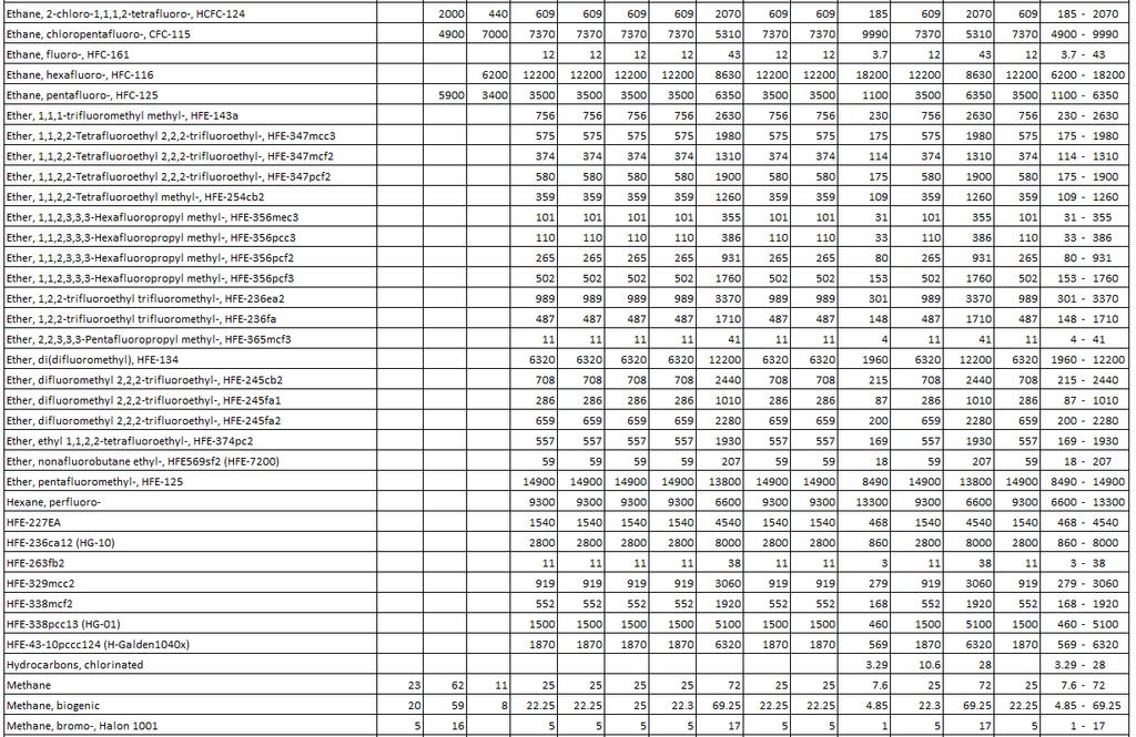
110 111

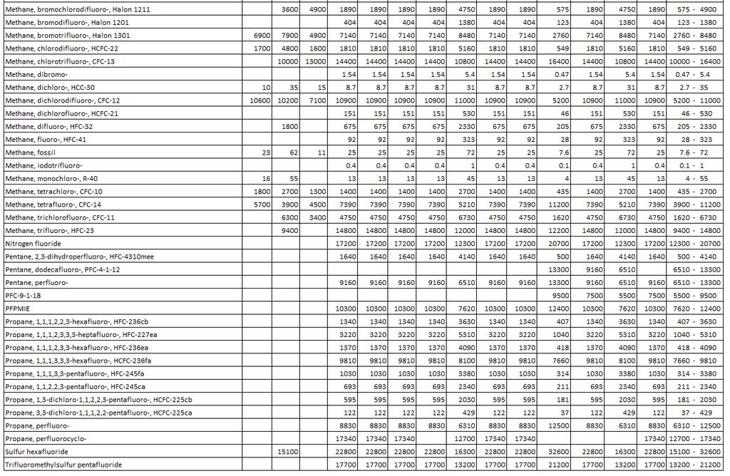
111 112

112 The observed high variability in the GW characterization factor values is somewhat unexpected because compared to other impact categories, the GW category is considered to be a relatively well-developed category. The estimation method for the GW category was assumed to be developed from one research agency, the Intergovernmental Panel on Climate Change (IPCC), and accepted by most of the methods. Thus, the coverages of substances were expected to be identical or at least similar between different methods. However, the results show that some methods have much smaller numbers of substances, such as BEES, CML2001, and Eco-indicator (which I stipulate are relatively older, but are still widely available in LCA software tools). No method includes all substances listed in Table 4-2. The ILCD method, for example, includes six substances that are not included in any other methods; yet it does not include Perfluorocyclopropane, a substance that is included in most of the other methods. Apart from the differences in the coverages of substances, the characterization factors also vary significantly across methods. This variability is beyond the variability expected from using different specific global warming timeframes. For example, there are six different values for Chloroform from 14 methods while the GW metric is defined at 20, 100, and 500 years. 4.3 Variability in the impact assessment results in the US LCI database Differences in the coverages from substances, and differences in the characterization factors are two sources for the variability in the LCIA results. A third source of variability is from differences in inventories that are connected to LCIA methods. The number of included substances in the inventory affects the LCIA result. This section evaluates the effects from the coverages of these GW substances in life cycle inventories. The 2701 elementary flows in the US LCI database include potential substances in each impact category. The purpose of this section is to identify these substances by matching their information with the elementary flows and substances provided in each category. The information includes the names of the materials or emissions in the elementary flows, as well as two other restrictive elements: compartments such as air, water and soil, and by impact regions such as lake, and river. As an example, Table 4-3 shows all elementary flows for Mercury in the US LCI database, specified to compartments and impact regions. Matlab software was used for the matching between the 113

113 information in the elementary flows and the substances in each category (code available in the Appendix), by the names and other restricted information. In some cases, the substances provided in impact categories are not specified by impact regions and compartments. Current practice is to apply the substances and their characterization factors in an impact method to all possible regions and compartments in the elementary flows. For instance, in the Ecoindicator 95 method, Mercury emissions to air is not regionally specified in the heavy metals impact category. The substance and its characterization factor are applied to all US LCI mercury flows to air (No. 1398, 1403, 1404, 1405 and 1411 in Table 4-3). On the other hand, when a substance provided by an impact method is regionally specified, an elementary flow in a LCI database should have the same impact region considered as a match. For example, in the ReCiPe Midpoint method, one impact region for Mercury to soil is forestry. As shown in Table 4-3, in the US LCI database, Mercury does not have forestry as one of its impact regions, indicating that the substance from the ReCiPe Midpoint method does not match any US LCI elementary flow. Table 4-4 shows the all GW substances in the US LCI database. Thirty five out of the 110 GW substances shown in Table 4-4 were identified as elementary flows. These GW substances were not regionally specified in the methods and applied to all elementary flows with the same chemical names. Thus, 94 US LCI elementary flows specified by impact regions were identified as matches. 114

114 Table 4-3: Elementary flows for Mercury with different impact regions and compartments in the US LCI database Flow No. in USLCI Name Impact region Compartment Unit 1398 Mercury unspecified air 1399 Mercury unspecified water 1400 Mercury industrial soil 1401 Mercury ocean water 1402 Mercury agricultural soil 1403 Mercury high population density air 1404 Mercury low population density air 1405 Mercury stratosphere air 1406 Mercury ground- water 1407 Mercury ground-, long-term water 1408 Mercury lake water 1409 Mercury river water 1410 Mercury unspecified soil 1411 Mercury low. pop. air 115

115 Table 4-4: GW substances in the US LCI database and their characterization factors in different methods. 116

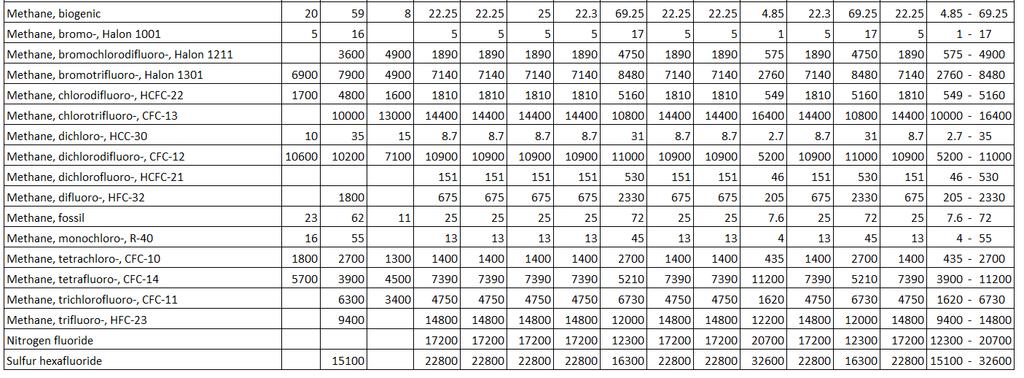
116 117

117 The number of substances for the five chosen impact categories are shown in Table 4-5. The first row in Table 4-5 shows the numbers of substances summarized from all impact methods for each category and the corresponding compartments (e.g., as described above there are a total of 110 distinct global warming substances across all methods considered). The third row represents the numbers of chemicals in each category that are included in the USLCI elementary flows. The forth row shows the number of elementary flows that have the same name with the substances in each category. Finally, the last row shows the total number of US LCI elementary flows classified by the compartments in the second row. The US LCI database classified 1030 elementary flows with compartment air, 237 with soil, and 924 as water. The results show that considering all five impact categories (the last column), around 60% (938 out of 2191) of the US LCI elementary flows are not substances in any of these categories, resulting in zero impacts. In addition, for each impact category, different methods provide different numbers of substances, resulting a range of number of substances covered (row 3). The ranges are generally large. For example, ozone depletion method has a number of matched substances vary between 6 and 25, indicating using one method can result in the neglect of 75% substances provided in another method. Table 4-5: Summary of the number of substances and matching elementary flows in five selected impact categories for the US LCI database. Number of substances from all methods Compartments for the substances Matched substances (compartment specified) Maximum number of matched elementary flows considering all impact regions GW Ozone Depletion Acicification Eutrophication Ecotoxicity All five categories Air Air Air, water, soil Air Air, water, soil Air, water, soil Number of elementary flows

118 The approximate 60% of exclusion of substances can be due to different reasons. First, possible cutoff criteria can cause neglects of emissions; the emissions that are smaller than the cutoff value are not reported in the inventory. Second, some particular substances are simply not emissions in the production. To better understand the reasons of the exclusions, based on individual industries and processes, I applied other data sources as reference to identify whether there are data gaps in the inventories. 4.4 Validating substances coverages and variability in the impact assessment results based on individual processes In the previous section, I listed the differences between the number of substances in the impact methods and in the US LCI database. The results showed that the differences can be large, in that the database may currently lack information on a large number of substances with known impacts. It is reasonable that there are more substances included in impact assessment methods than the numbers of substances emitted from production since data comes from many individual processes, each of which could in fact not have emissions of such substances. However, if results from another data source shows that the emissions likely exist but are not covered in the US LCI process, it means that there is a data gap and the inventory should be updated to include the emissions. To demonstrate the idea of using these references to determine whether there are data gaps, in this study, I used the global warming impact category as an example, because the data for this category are currently available. The methods can be applied to other impact categories as more third-party data can be acquired. The US EPA s Greenhouse Gas Reporting Program (GHGRP) 2 provides annual Greenhouse Gas emissions data from large emitting industries. In 2009, the US EPA published a mandatory reporting rule for greenhouse gas emissions. It regulated that facilities in the US should report any emissions that are more than 25,000 metric tons carbon dioxide eq per year. Since then, the US EPA collects reported emissions from these facilities and provides the data to the public. The latest data are from 2015, for 32 industry types. These data were used in this study to identify greenhouse gas emissions from different industries and as a reference to identify possible data gaps in the US LCI database. 2 US EPA Greenhouse Gas Reporting Program. accessed

119 Based on the data provided by GHGRP, the greenhouse gas emissions reported by each industry under the mandatory reporting rule are summarized in Table 4-6, cells with EPA indicate that there were more than 25,000 metric tons of carbon dioxide equivalent greenhouse gas emissions from various industries (EPA provides 32 industries, for simplicity, only industries covered in the US LCI database are listed in the table). The summarized results from the EPA reports show that carbon dioxide, methane and dinitrogen oxide are reported in the emissions from all industries, while the other six greenhouse gases are reported in only in metal, chemical, and electronic manufacturing industries. The table, lists the inclusion or exclusion of the greenhouse gases in the US LCI database; the red cells indicate the EPA reported emissions that are excluded from any US LCI process within the same industry. The result shows that there are data gaps for some industries in the database, especially in ethanol production and electronics manufacturing industries; the non-zero values are reported to EPA from these industries, but the substance are not included in the processes inventories. For example, EPA requires metal production industries to report perfluorocarbons; however, among the 22 US LCI metal processes, none have perfluorocarbons as outputs. The exclusion of these substances could be caused by the time differences between the inventories reported and the release of the mandatory reporting rule; some of the inventories were reported before 2005, thus the emissions reporting were not regulated by the rule. These old inventories can be improved referencing the rule. However, the exclusions of global warming substances indicate possible exclusion of substances from other impact categories, and currently no reference can be found to identify possible gaps. Future studies can aim to solve these problems by identifying impact substances from industrial emissions. 120

120 Table 4-6: Mandatory Greenhouse gases reported to the US EPA GHGRP for each industry. Cell listed as EPA are emissions reported under the mandatory reporting rule. Cells highlighted with red color are emissions that are not included in any of the US LCI process within each industry. The evaluation on the industrial level provides a high level summary of the inclusion of global warming substances. A detailed level analysis was also performed to understand the inclusion of US LCI processes. For simplicity, the matrix method is applied. Considering all substances summarized from the 14 different impact methods, the values in the B matrix were used to identify whether a process had certain substances in the direct emission. Each row in the B matrix, found in Equation 3, represents an elementary flow, which is a direct input or output for the processes in the columns. For each column, non-zero values in the rows represent direct emissions from identified substances in each process. Thus, identifying the non-zero values in the substance rows efficiently leads to the substances from each process. The zero values were assumed to have zero effects, thus resulting in no corresponding impacts. Figure 4-2 shows the ranges in number of GW substances for the US LCI gate-to-gate processes. Using their maximum values, these ranges are sorted by the process having the largest number of GW substances (left) to the smallest (right). The two values for each process are the maximum and minimum number of substances summarized from 14 impact assessment methods (shown in Figure 4-2). For example, in Figure 4-2, process number one had a range of identified substances between 11 and 15; this range resulted from using different impact methods. The cut-off processes do not have any output component; thus, they were not shown in Figure 4-2. Cradleto-gate processes were also excluded in Figure 4-2, because their emissions are not exclusively 121

121 direct emissions. Figure 4-2 also omits processes without GW substances. The results show that the discrepancies between the maximum and minimum numbers can be large. Only 314 or 25% of the 876 cradle-to-gate processes had more than one GW substance, and 523 processes do not include any GW in their inventories. As show in Figure 4-2, the processes with the largest numbers of GW substances are fuel combustion processes. There were some instances in which the number of substances was small or even zero. This lack of substances induces a small or zero value for the direct GW impact results in most of the processes (i.e., it would report that the process has no global warming impact). The reason for the lack of substances can be traced to the inventories of the processes. Most processes do not include GW substances in their inventories. It is possible that the processes do not have GW emissions. For example, the electricity, US, grid mix process is a mix of electricity generated by different types of fuels. In this case, generating grid electricity does not involve any real production (no emission is produced from the process). However, these special cases only apply to a small part of the processes, not to all the 523 processes. GW substance emissions may also be excluded from the inventory when they are outside the system boundary of the LCA studies. This exclusion can result in ignoring impact values in the results. When the system boundary is set, the inclusion/exclusion of certain emissions is often based on benchmarks referred to as cutoff criteria. The cutoff criteria specify a boundary using mass, energy or economic value, rather than impact results. Thus, small emissions from substances are more susceptible to being excluded from the inventory. I will discuss cutoff issues more in the next section. 122

122 Figure 4-2: Numbers of Global warming (GW) substances in the gate-to-gate process from the US LCI database. The processes were sorted from the largest number of substances (left) to the smallest (right). The two values for each process are the maximum and minimum number of substances in 14 popular impact assessment methods (see Table 4-2). The cut-off processes in the US LCI database are not shown in this figure, as these processes do not have any output component. Also omitted are the processes without GW substances after No The first 10 processes names are shown in the table. So far, I have identified the direct emission substances from each process in the US LCI database. Now I focus on the indirect/upstream emission substances and their impacts from each process. The indirect emissions for each process were obtained from the g vector. After identifying the substances, the final ranges of impact results were computed from their corresponding characterization factors. The differences observed in the impact results were due to the variabilities in the characterization factors, and the number of substances covered in each method. 123

123 In the direct analysis, I found 548 processes with no GW substances (from any GW methods) in their direct emissions (i.e. in the B matrix). In the direct and indirect analysis, 268 out of these 548 processes include GW substances in their upstream (i.e., in their g vectors). As an example, Figure 4-3 summarizes the occurrence GW substances for the processes with the top ten highest number of GW substances in their direct inventories (i.e., the first ten processes listed in Figure 4-3). The non-zero substances corresponding to direct and indirect emissions are displayed separately and highlighted in orange; red border cells are reported as non-zero values by the EPA GHGRP. The results indicate that 1) more substances are found in the total emissions; 2) some substances are widely included, such as fossil carbon dioxide; 3) some GW substances reported in EPA GHGRP are not included in some of the processes inventories. 124

124 Figure 4-3: Non-zero values for the US LCI processes that have the largest numbers of global warming (GW) substances. The marked cells in the tables represent non-zero values. Cells with red borders are reported as non-zero values by the EPA GHGRP. The direct and indirect tables were obtained from the B matrix, and g vector for each process respectively (the non-zero values are highlighted in orange). Ten example processes with only one direct GW substance in the B matrix columns are shown in Figure 4-4. Perhaps contrary to expectation, when a process has only one GW substance, it is not necessarily carbon dioxide, but can also be dinitrogen monoxide (N 2 O).The results also show that the numbers of substances in the g vector for the same process are larger, further indicating that indirect emissions are important to the impact results. Figure 4-3 and Figure 4-4 highlight the substances included in the process inventories. For processes with either the top 10 highest or lowest numbers of GW substances, when EPA s GHGRP is used as a reference, potential data gaps are found in in the processes inventories. Though the total effects cover more substances, the missing substances are still excluded from the inventories, indicating the missing substances are not included in the inventory of any upstream inputs. Excluding these substances results in missing impact values; this is an issue in LCI databases, especially for the processes that have small numbers of GW substances. Addressing this issue can improve the quality of databases and facilitate better LCA results. 125

125 Figure 4-4: Non-zero values for the US LCI processes that have only one global warming (GW) substance. The highlighted cells in the tables represent non-zero values. Cells with red borders are reported as non-zero values by the EPA GHGRP. The process number corresponds to the x-axis in Figure 4-2. Next, using Equation 3 and Equation 5, I calculated the total impact assessment results per functional unit for each of the 876 gate-to-gate processes in the US LCI database. All 14 methods 126

126 were used in the estimation. Again, Matlab software was used to match substances. Among the 876 gate-to-gate processes, 608 have non-zero GW impact results which are graphed below. Of these 608 processes, Figure 4-5 shows results for the 50 processes with the largest total GW impact values per functional unit. The total impact values for each process were calculated based on 14 different GW methods, as shown in the legend. Each row in the figure represents the 14 total emissions from one functional unit production of a process. The displayed processes were sorted by the maximum GW impact value calculated from all methods. Figure 4-6 shows the results for the remaining 558 non-zero-impact processes. The processes with the 10 largest total GW impact values are different than the processes with the 10 largest numbers of GW substances in Figure 4-3, because the GW impact values are affected by the characterization factor values for the substances, whose values can differ by three orders of magnitudes between different substances. In general, the GW results are similar across different methods. Among the 608 processes, 517 have less than 5% absolute departure from the average value (i.e., the difference between the maximum or minimum value and the average is less than 5%). There are some big outliers from two impact methods. No. 17 to No. 23 on the x-axis, for example, have larger values calculated from the Greenhouse gas protocol method (light blue squares) than using the other methods. On the other hand, processes No. 305 to No. 310 have larger values from the CML 2001 method compared to the other methods (Figure 4-6). 127

127 Figure 4-5: GW values in CO 2 eq per functional unit, from 14 impact methods, marked by the different symbols described in the legend. Processes No.1 to No.10 are shown on the left, and processes No. 11 to No. 50 are shown on the right. The processes are sorted by total impact results including direct and indirect impacts. The first 10 processes names, industrial categories, functional units, and original index numbers from the US LCI database are listed in the table. 128

128 Figure 4-6: GW values in CO 2 eq per functional unit from 14 impact methods for processes No. 50 to No The processes are sorted from high to low by the total impact results including direct and indirect impacts. Other processes with zero GW impact from any of the methods are not shown. 129

129 The processes provided in Figure 4-5 and Figure 4-6 were sorted to visualize the uncertainties in all processes; however, the functional units of these processes are different, making comparisons of uncertainties between processes impossible. In addition, the processes from the same industry could have similar impacts. Thus, I also grouped the processes from the same industries together to enhance the interpretation of results. Figure 4-7, Figure 4-8 and Figure 4-9 provide GW impact results for three example categories: transportation, electricity, and plastic material. These three categories are chosen as examples because their processes have relatively similar attributes, such as upstream flows and downstream uses. The results show that within the three categories, the maximum and minimum impact values are generally from the same impact methods. IPCC a often provides the largest GW impact, while ReCiPe Midpoint (I) results in the minimum impact value. These two methods cover the same numbers of substances, thus, the differences in the impact values were due to the differences in the characterization factor values. For the GW impact category, different time intervals is one of the reasons for the discrepancies in the impact results. As shown in Figure 4-7, Figure 4-8 and Figure 4-9, for most of the processes, clearly there are three sets of GW impacts. They are the results from three GW time intervals: short (20 years), medium (100 years), and long term (500 years). The differences in the characterization factors are the sources of the variances in these three sets: for some of the substances, such as methane, the short term characterization factors are larger than the long term ones. This difference regarding the time span is due to the lifetime of a substance: if the substance can be removed from the atmosphere in a fairly short amount of time (less than 500 years), its characterization factor value decreases over years. Therefore, the impact results calculated from impact methods using different GW time intervals are different, they should be separately and clearly listed when provided to the users. In this study, I believe showing all results together with clearly listed legends can help the users to understand the differences caused by choosing different impact methods; listing all impact results together can als o provide the differences caused by using different time intervals. When the methods are incorporated into LCA software, the results can be improved by introducing user interface features. In short, the software should aim to provide all possible impact results from different impact methods and clearly separate the results from different time intervals 130

130 Figure 4-7: GW impact values in CO 2 eq per ton-km for 190 transportation processes in the US LCI database. Figure 4-8: GW impact values in CO 2 eq per kwh for 98 electricity processes in the US LCI database. 131

131 Figure 4-9: GW impact values in CO 2 eq per for 23 plastic material processes in the US LCI database The results above were high-level summaries across all US LCI processes to demonstrate the variability in results from various GW methods. Showing the detailed results calculated from LCIA methods can help LCA practitioners to understand the uncertainties caused by selecting different impact methods, which is more easily understood when considering a single process (which is the type of decision a practitioner would make when putting together a study). As such, Figure 4-10 shows the GW impacts calculated from 14 different methods for an example process, Crude palm kernel oil, at plant. The process was chosen because compared to most of the processes, it has a larger range of GW impact values. Among the 14 methods, two methods (CML2001, and GHG Protocol) cover different substances (see Table 4-6). 132

132 Figure 4-10: Total GW impacts for the Crude palm kernel oil, at plant process calculated from 14 different methods. Two of the 14 methods listed in the figure have different covered substances (The markers are the same as in Figure 4-5). Table 4-7: GW substances for the Crude palm kernel oil, at plant process, and impacts for the substances calculated from 14 impact methods. The cells with larger values are highlighted with darker bacround. Thus, the discrepancies between the remaining 12 methods are caused entirely by the differences in their characterization factors. As shown in Table 4-6, the larger value from the GHG Protocol method was caused by Carbon dioxide, biogenic, a substance that was not included in any other methods. Because the impact value for this substance is 3.3 CO 2 eq, larger than the total GW impact calculated from all other methods, it causes an outlier in the total GW impact values. If this substance was not included, the GW impacts calculated from the GHG Protocol method would be CO 2 eq, which falls in the lower end of the impact range. On the other hand, the CML2001 method included two substances ( carbon monoxide and carbon monoxide, fossil ) that were generally excluded from other methods. Here, by saying excluded, I mean that 133

133 the chemicals were not shown in the list of substances of the method. However, because the impact values from these two substances were not large, the total impact results from the CML2001 method were within the range of other methods. It can be concluded that for this process, the discrepancies of the total impact results are caused by differences in: 1) the total emission values for the characterized substances in the g vector; 2) the coverages of substances in methods; and 3) the differences in the characterization factor values of the substances. From the example in Figure 4-10 and the results from all US LCI processes (Figure 4-6), I can generally conclude that the outliers of the impact results are often caused by the inclusion of certain unusual substances in a particular method. The ranges in the impact results can be attributed to the differences in the characterization factors. It would be useful to incorporate visualizations, like those in Figure 4-10 and Table 4-6, as readily available tools in LCA software. These visualizations improve the understanding of the LCIA results by showing the main sources of discrepancies. I believe that these visualizations would enable LCIA users to make more robust decisions. To better understand the correlation between the numbers of substances covered and the total impact results, I performed a regression analysis to test the relation between the numbers of characterized substances and the impact results. In matrix-based models, the resulting emissions are calculated from a dot product between a vector of substances and a vector of processes (Equation 3). Suppose both vectors have p elements, where p is the number of substances from an environmental impact. To evaluate the scenario uncertainty, I considered alternatives for the vector of substances. However, sometimes the vector of substances has several missing entries; this number often changes with different scenarios. The proportion of completeness is defined as 1-(number of missing substances divided by p). Algebraically, the dot product is a sum of entry-wise products in two vectors; all things equal, this sum will be smaller if some entries are zeros. I decided to test the extent to which the results are affected by the proportion of substance completeness in our analysis. See Figure 4-11 for the case of Global Warming, three other environmental impacts are considered in Figure S1 of the Appendix. I first computed the proportion of substance completeness for multiple scenarios 134

134 (denoted by marker color). Then I evaluated the resulting emissions under different processes (608 in this case). Because different process result in distinct magnitudes, I standardized the results of each process, i.e. I subtracted the average and divided by the standard deviation. The null hypothesis I tested is that a constant model is better than a linear model. A constant model (zero slope) represents the absence of a linear relationship between the results and the proportion of completeness. Using weighted least squares regression, I rejected the null hypothesis in favor of a non-zero slope (F statistic=479, df=8510, pvalue<0.001). The regression weights were inversely proportional to the variance of repeated results within the domain of substance completeness proportion. Figure 4-11: Testing the relation between the results from Global Warming and substance completeness proportions. The marker color indicates different alternative scenarios. The black line is the fit obtained from a linear weighted least squares regression. Results from the regression analysis reject the null hypothesis in favor of a correlation between the numbers of substances with the impact results. Similar results are shown for other three impact categories (Eutrophication, Acidification, and Ozone depletion). From the regression figure, it can be seen that CML2001 and GHGProtocol methods result in higher GW impacts. Considering the results in Table 4-6, it could be possible that the larger values are caused by a few substances 135

135 that are excluded from all other methods, such as the biogenetic carbon dioxide. It will be helpful to quantitatively identify the uncertainty from the coverage of substances and the differences in the characterization factors. However, the number of substances covered in the US LCI inventories are not large enough to include most of the substances provided by each impact method; most processes cover similar substances. Thus, the results of regression test (and other potential methods) are determined by only a few exceptions, such as the substances shown in Table 4-6. The conclusion made based on these results can be arbitrary. Future studies can focus on improving the estimation with more completed inventories. 4.5 Impact based inventory reporting criteria As discussed previously, most inventories in the US LCI database do not have characterized substances in each impact category, and some of the exclusions can be confirmed as data gaps by introducing other data sources, such as EPA GHGRP. This lack of information results in potential neglects of impact values in the LCA results. Here, I introduce a new inventory reporting criterion. The criteria are developed with respect to the potential environmental impacts and informed by the analysis above. I believe this new impact based criteria can help LCA studies to build more robust inventories. The proposed criteria are estimated based on the characterization factors of a substance and the knowledge of existing impacts from processes. Similar to the traditional cutoff criteria estimation, a certain ratio is used to regulate the minimum report impact value. The ratio can be defined according to the purpose of the studies, such as 5% (less strict), 1%, or 0.5% (stricter). Then, using the corresponding characterization factor, the minimum report impact value is converted to physical units of emissions. The estimation method is described in Equation 6. The criterion was the result of the impact values and the substance s characterization factor value. In Equation 6, T i is the new impact based criterion for a certain substance i, r is a constant ratio, P is the environmental impact result for the process under study, and CF i is the characterization factor. Equation 6: T i = r P CF i 136

136 In this study, I determine P based on the impact values from existing LCA studies. For instance, the GW impact from the Electricity, bituminous coal, at power plant process is currently around 1 CO 2 eq per kwh generation. Our new criteria rules that any substances with more than 0.05, 0.01, or CO 2 eq (5%, 1%, or 0.01% of the 1 CO 2 eq, respectively) GW impact should be ensured to be included in the inventory. Table 4-7 shows the criteria estimation for the Electricity, bituminous coal, at power plant process. The criteria for all GW values were calculated referencing the current impact values in the bituminous coal electricity generation. In the current US LCI database, producing 1 kwh of electricity generated from bituminous coal results in 0.99 CO 2 eq GW impacts, this value is used for P in Equation 6. To evaluate the results in two different situations, the ratio r was defined as 1% and 5%. Because the maximum across all CF i s results in the most extreme case of impact result, the maximum GW characterization factor (CF) values from 14 methods were used to estimate the strict criteria. The average characterization factor values were used for general criteria estimation. 137

137 Table 4-8: Maximum characterization factor value and new cut-off criteria for each substance. Cut-off criteria were based on 5% and 1% of total GW for 1kWh Electricity, bituminous coal, at power plant The first 34 GW substances are shown as examples. 138

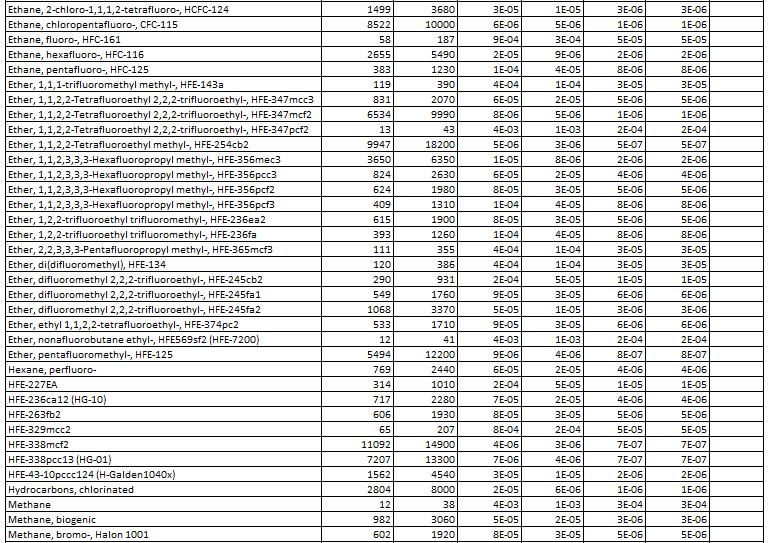
138 139

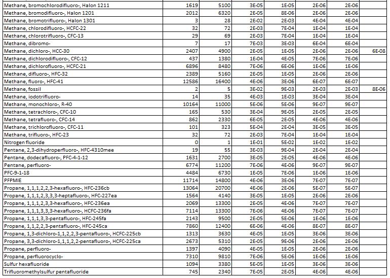
139 140

140 Under the impact based inventory reporting criteria, the data reporters of LCA studies can be motivated to provide more potential substances in the inventories. In this way, the inventories can be improved and larger impact results can be expected. However, it is possible that after including more emissions, the environmental impact rises significantly, making the 1% or 5% total impact criteria larger than the original value. The larger criteria can result in the exclusions of emissions that are currently included. As a result, the new impact based criteria needs to be improved. However, based on the inventories in the current US LCI database, I am not able to decide how many new substances are going to be included and how much they are going to contribute to the total impact. Thus, the impact based criteria requires continued development. 4.6 Discussion This study compared different commonly used impact assessment methods along with their impact categories. The substances in the elementary flows were identified to show the coverages of substances in LCI databases and it was found that different impact methods provided different coverages of impact categories and substances, as well as different characterization factor values. Considering five impact categories, around 50% of the US LCI elementary flows are not substances in the impact methods. Based on each process, when another data sources is used as a reference, some GW substance are missing from the inventory. These results could help the LCA practitioners better understand current situations in LCIA analyses. The substances in the indirect effects in some cases can be much larger than the ones in the direct effects. This shows the effectiveness of a matrix-based LCA model in estimating indirect effects and impacts. The total (direct and indirect) impact of a gate-to-gate process is approximately the same as the impact of cradle-to-gate processes for the same product. This suggests that cradleto-gate processes are not necessary when using a matrix-based model because the matrix model can sufficiently provide all upstream effects and impacts. To conduct an LCIA, the LCA practitioners often select one impact method and rarely compare results from different methods. Typically, there is no awareness of what the results might be under different methods. In LCA software, the choice of the method is left to the discretion of the user. Consequently, if the users do not understand the potential impacts of choosing one method 141

141 over another for the particular analysis, then one could accidently choose an inappropriate method. For example, a method with inappropriate GW time interval might be chosen for a study with a particular time scope.. There is also a danger of confirmation bias. The users could choose a method that supports the preconception and fails to investigate other possible alternatives. The consequences can be problematic. The impact results calculated from different methods show that the discrepancies can be large. The sources of discrepancies can be traced to different coverages and characterization factors in the substances. The wrong choice of a method may result in wrong decisions. To overcome these issues, I recommend new visualization tools that provide a rich description of the LCIA methods and show results comparing different impact methods. By providing readily available visualization tools in LCA software like SimaPro, the users would be able to make more robust decisions based on the observed ranges. I showed that substances with large characterization factors are not necessarily included in the inventory of a process. To understand the exclusions, I used EPA s GHGRP as a reference to identify possible data gaps in the US LCI inventories. The results show that some processes have missing GW substances; this issue should be addressed when updating the database. No other reference can be found to identify possible gaps in other impact categories; however, the database should focus on improving the inventories to avoid data gaps in the GW category. A more specific cutoff criteria with respect to impact assessment results should be encouraged to LCI data reporters. 142

142 5. Chapter 5. Conclusions and future work In this chapter, I provide brief answers to the research questions listed in chapter 1. I also provide a general conclusion, discussion, and future work. 5.1 Research question and answers Chapter 2. Parameter uncertainty in the EIO-LCA model What are the uncertainty ranges of direct and indirect life cycle energy consumptions over the supply chain of the U.S. industries based on economic input-output models with public available data? In chapter 1, the uncertainty of energy consumptions in the US industries were evaluated based on multiple data sources and range methods. The results show that the uncertainty of direct life cycle energy consumption in the US industries is generally around 50%, with some extreme cases that reach over 40 times the default value. Considering the indirect energy consumption, the overall uncertainty of each industry is smaller. The total energy consumption, considering all 428 industries, is generally within -40% to 40%, with a few extreme cases that have over 4 times more impact. What is the impact of each individual industry s uncertainty on results of other industries? Based on the uncertainty results from the first research question, the industries with large discrepancies in the direct energy consumption were identified. The impacts from these industries on the total energy consumption was estimated. The results show that the uncertainties from each industry affect the uncertainties in the model differently. The top five industries that have the strongest impacts are: power generation and supply, petroleum refineries, oil and gas extraction, iron and steel mills, and coal mining. Which industries have the largest uncertainties in the model? How to reduce the uncertainties of these industries? 143

143 The results show that Coal mining sector and Petroleum lubricating oil and grease manufacturing sectors have the largest uncertainties (over 500% larger compared with default) in the direct energy consumptions. The total energy consumption value for Coal mining varies from 5 to 70 TJ/M$, and Petroleum lubricating oil and grease manufacturing varies from 3 to 110 TJ/M$. The reasons for their large uncertainty in total consumption values can be traced to the large discrepancies in the direct consumption, which are caused by problematic documented data. Chapter 3. Data analysis in the US LCI database and scenario uncertainty in matrix-based models In the current US LCI database, how many processes flows contribute to the indirect environmental effects when applied to matrix-based LCA models? In this chapter, I assume that the gate-to-gate processes restricted by two criteria can contribute to the indirect effects when incorporated to matrix-based LCA models. The two criteria are: 1) processes with at least one upstream or downstream connection; and 2) processes that include energy and transportation in their direct inputs. By evaluating each process individually, I found that there are only 61 processes that meet these criteria. This indicates that less than 5% of processes in the US LCI database contribute to the indirect effects in matrix-based LCA models. What are the total CO 2 emissions ranges from US industrial processes by considering different scenarios from current process-based life cycle inventory databases? The scenario uncertainties for the processes in the US LCI database were analyzed by using alternative inputs as different scenarios. The results show that by using different utility inputs as alternatives, the scenario uncertainties are generally within -20% and 20%, with some outliers. What are the ranges of total CO 2 emissions ranges from aggregated US industrial processes calculated from current process-based life cycle inventory databases? 144

144 Bigger scenario uncertainties are observed by using different processes as alternatives within the same industrial category. One example industry shows that the CO 2 emissions for 1 of industrial product can vary between 0 and 400. Chapter 4. LCIA uncertainty in a process-based LCI database In current LCIA methods, how many substances are covered? How many of these substances are included in elementary flows in the US LCI database? Does the US LCI database have enough flows that are characterized in impact assessment methods to build a robust inventory? I examined the 50 LCIA methods summarized in the SimaPro software. The results show that the numbers of substances across impact categories vary significantly: from as few as 18 substances to as many as 30,514 substances. Within the same impact category, the numbers of substances covered by each method are generally similar, with a few exceptions. For each of the five categories used in this study, less than 50% of its characterized substances were included in the US LCI database. This result indicates that the US LCI database does not have a robust inventory for LCIA studies. For processes in current process-based LCA databases, what are the uncertainties of direct and indirect environmental impacts caused by different impact characterization factors used in LCIA? The results generally show that 80% of the gate-to-gate processes have less than 5% uncertainties, with respect to choosing different impact assessment methods. However, these small uncertainties are estimated based on insufficient US LCI inventories, the uncertainty results do not justify small uncertainties in the model. What are the contributions of different characterization factor values and coverages of substances from different methods to the LCA result? The results show that based on individual cases, the different coverage of substances does not have strong impacts on the total results. However, a statistical study rejected the 145

145 possibility of independency in favor of a linear relationship between the number of substances and the total impact values. What should be the new reported value in LCI for different substances considering impact assessment results? I propose a new minimum data report criteria based on LCIA results. The proposed criteria regulates that all emissions from substances should be taken into consideration and measured before reporting an LCI database. An example result show that considering global warming impacts, the minimum reported value (by mass) can be as small as 5E-7 for 1 electricity production. However, this value is larger than the minimum reported value for the same process in the current US LCI database. 5.2 Conclusion This dissertation examines the uncertainties in the matrix-based LCA models. Three types of uncertainties (parameter, scenario, and model) are considered and evaluated based on two types of matrix-based LCA models: the input-output, and process-based LCA. With a range method, I estimated the uncertainties of two environmental effects (greenhouse gas emissions and energy consumptions) and five environmental impacts (global warming, ozone depletion, acidification, eutrophication and ecotoxicity) in matrix-based LCA models. In chapter 2, I examine the parameter uncertainty and use the range method to propagate the uncertainty in the EIO-LCA model. Publicly available data sources and value-converting assumptions are used to estimate the parameter uncertainties in the direct industrial energy consumption. The total (including indirect) energy consumption ranges are estimated through the matrix-based LCA model. The results show that the parameter uncertainties can be large in IO based LCA models. The uncertainties can be traced to individual industries and reduced by improving the raw data. 146

146 In chapter 3, I estimate the scenario uncertainties in matrix-based LCA by using alternative inputs in the US LCI database. By examining the processes, I find the US LCI database fails to provide well-connected processes to take full advantage of matrix-based method. Based on our definition, less than 10% of the processes in the database are well-connected so that they contribute to the indirect environmental effects when incorporated to matrix-based LCA models. I also estimated the scenario uncertainty in the model with the range method. The results show that the scenario uncertainties of each process caused by using different electricity or transportation inputs are smaller compared to the parameter uncertainties estimated from chapter 1. However, the industrial level uncertainties are much larger, due to the incompleteness of the database. The model uncertainty in matrix-based LCA models is addressed in chapter 4. Model uncertainty refers to the differences in LCIA methods. The same range method is used to estimate the variances in the environmental impact results for each US LCI process. In the LCIA methods selected for this study, I compare the differences in the coverages of substances and characterization factor values, and identified the number of substances in the US LCI elementary flows. The results show that the model uncertainty due to different choices of impact methods in the US LCI database is small, negligible in most of the processes. However, as the US LCI database does not have a robust inventory to support LCIA analysis, most of the processes do not include enough substances in their inventories. The impact values are the results from a few substances in the database, thus, I cannot conclude that the difference in impact methods has negligible effect on the total impact results. Aiming to improve the database, I propose new criteria to regulate minimum report inventory values. The criteria are estimated based on the impact results as well as the characterization factors for each substance. The parameter, scenario, and model uncertainty together contribute to the uncertainty in matrixbased LCA models. The results in matrix-based LCA models generally show considerable uncertainties in the total energy consumption and GHG emission across most US industries. However, current LCA software fail to provide users with these uncertainties. The users often ignore the uncertainties in the data and model. LCA software is developed to assist LCA studies, which are in turn designed for making decisions based on quantitative results. When the 147

147 uncertainties are ignored, LCA software can only provide deterministic results that lead to subjective decisions. Furthermore, the analyses on the US LCI inventories indicate a potential problem in the LCI databases. The LCI database is widely applied to matrix-based LCA models for estimating total environmental effects and impacts. However, I find several problems in the current LCI database. These problems limit the advantages of matrix-based LCA models. The two biggest problems are inconsistencies in processes and incomplete inventories. Inconsistencies in processes are generally caused by including processes with different system boundaries in the same database. For example, cradle-to-gate processes and gate-to-gate processes are both included in the database. The incompleteness in the inventories can be found in both product flows and elementary flows. Processes are generally not connected in the database, resulting in the neglect of indirect effects. On the other hand, though the total number of elementary flows covered in the database is large, most of the substances that generate large environmental effects are excluded from the inventories. These types of incompleteness results in ignoring important effects and/or impacts; however, the LCA practitioners are often unaware of these problems when using the database. In conclusion, the uncertainties in matrix-based LCA models can be large; however, they are easily ignored by LCA practitioners. Future LCI databases should focus on including better inventories as well as uncertainties in the inventories. LCA software should aim to provide better uncertainty estimation methods and results to the users. 5.3 Future work Analyze the uncertainties of other environmental effects in the matrix-based LCA models In this dissertation, the uncertainties in energy consumption and carbon dioxide emissions were analyzed for EIO-LCA model and the US LCI database, respectively. The same uncertainty estimation method introduced in this study can be applied to other environmental effects to both of the models as well as other matrix-based LCA models. For example, the uncertainty of carbon dioxide emissions in the EIO-LCA model can be evaluated next. 148

148 5.3.2 Quantify the relationship between the technology matrix and the environmental matrix In this study, the uncertainties were separately evaluated for the technology matrix and environmental effect matrix. Due to the limitation of the database (only a few portion of the processes are connected), I have not traced the sources of the uncertainties to these two individual matrices. Future work can focus on quantitatively analyze the contributions from these two matrices to the overall uncertainty Estimate scenario uncertainty using other LCI databases The US LCI database was used to demonstrate the methods and results in this dissertation. Future work can focus on identify the problems and estimate uncertainties with other LCI database, such as Ecoinvent. Ecoinvent has more than 10 thousand processes and elementary flows, if these processes are better connected, there can be more scenarios available. For example, except utility and transportation industry, similar processes within metal, plastic material production industries can be used as alternatives Test the correlation between number of substances covered and the total impact results In this study, I tested the correlation between the numbers of substances and the impact results. The preliminary results were based on insufficient LCI data. Future work can repeat the same test on other LCI databases that include more substances. The conclusions from the regression tests could change. Furthermore, another parameter, the differences in the characterization factors can be used in the regression test. The results can provide quantitative conclusions on the effects of LCIA methods on a statistical perspective Improving the minimum report value criteria The minimum report value criteria introduced in this study need to be improved. More inventory data that covers more substances should be used for estimating the criteria. With the real-life inventory data, control tests can be performed to test how the new criteria impact on the report of new inventories; on the other hand, sensitivity analysis can be applied for analyzing the impact from the new reported inventory to the future updates of the criteria. 149

149 Appendix Table S1: IO industry code, name, and uncertainty ranges Sector No. IO No. Name Uncertainties A0 Oilseed farming 2% -83% B0 Grain farming 34% -78% Vegetable and melon farming 20% -54% Tree nut farming 14% -54% A0 Fruit farming 11% -55% Greenhouse and nursery production 101% -43% Tobacco farming 14% -79% Cotton farming 13% -73% A0 Sugarcane and sugar beet farming 55% -59% B0 All other crop farming 102% -55% Milk Production 18% -62% A0 Cattle ranching and farming 23% -78% Poultry and egg production 152% -55% A00 Animal production, except cattle and poultry and eggs 9% -71% Logging 0% -97% A00 Forest nurseries, forest products, and timber tracts 0% -89% Fishing 0% -100% Hunting and trapping 0% -76% Agriculture and forestry support activities 0% -69% Oil and gas extraction 13% -76% Coal mining 1251% -75% Iron ore mining 15% -48% Copper, nickel, lead, and zinc mining 29% -69% A0 Gold, silver, and other metal ore mining 77% -72% Stone mining and quarrying 92% -69% Sand, gravel, clay, and refractory mining 70% -48% Other nonmetallic mineral mining 75% -44% Drilling oil and gas wells 139% -94% Support activities for oil and gas operations 127% -95% A Support activities for other mining 135% -87% Power generation and supply 1% -33% 150

150 Natural gas distribution 0% -16% Water, sewage and other systems 0% -27% Nonresidential commercial and health care structures 18% -87% Nonresidential manufacturing structures 2% -87% Other nonresidential structures 33% -89% Residential permanent site single- and multi-family structures 27% -84% Other residential structures 28% -84% Nonresidential maintenance and repair 35% -89% Residential maintenance and repair 35% -92% Dog and cat food manufacturing 77% -10% Other animal food manufacturing 83% -9% Flour milling and malt manufacturing 80% -7% Wet corn milling 35% -46% Fats and oils refining and blending 80% -10% A Soybean and other oilseed processing 69% -16% Breakfast cereal manufacturing 73% -12% Beet sugar manufacturing 31% -34% A Sugar cane mills and refining 27% -28% Confectionery manufacturing from cacao beans 74% -8% Confectionery manufacturing from purchased chocolate 79% -8% Nonchocolate confectionery manufacturing 80% -8% Frozen food manufacturing 73% -10% Fruit and vegetable canning, pickling and drying 84% -10% Cheese manufacturing 80% -8% Dry, condensed, and evaporated dairy products 78% -10% A Fluid milk and butter manufacturing 89% -8% Ice cream and frozen dessert manufacturing 77% -5% Poultry processing 61% -15% A Animal (except poultry) slaughtering and processing 79% -9% Seafood product preparation and packaging 91% -9% Bread and bakery product manufacturing 90% -9% Cookie, cracker and pasta manufacturing 79% -8% Tortilla manufacturing 96% -10% Snack food manufacturing 79% -10% Coffee and tea manufacturing 80% -9% Flavoring syrup and concentrate manufacturing 83% -9% Seasoning and dressing manufacturing 74% -9% All other food manufacturing 92% -9% 151

151 Soft drink and ice manufacturing 63% -7% Breweries 58% -12% Wineries 77% -6% Distilleries 51% -11% A0 Tobacco product manufacturing 198% -49% Fiber, yarn, and thread mills 19% -20% Broadwoven fabric mills 21% -25% Narrow fabric mills and schiffli embroidery 39% -29% Nonwoven fabric mills 21% -32% Knit fabric mills 33% -28% Textile and fabric finishing mills 34% -30% Fabric coating mills 39% -32% Carpet and rug mills 29% -34% Curtain and linen mills 37% -30% Textile bag and canvas mills 41% -31% All other miscellaneous textile product mills 23% -34% Hosiery and sock mills 144% -16% Cut and sew apparel contractors 219% -13% Men's and boys' cut and sew apparel manufacturing 152% -14% Women's and girls' cut and sew apparel manufacturing 264% -18% Other cut and sew apparel manufacturing 119% -7% Accessories and other apparel manufacturing 338% -21% Leather and hide tanning and finishing 72% -16% Footwear manufacturing 65% -24% Other leather and allied product manufacturing 58% -42% Sawmills and wood preservation 19% -11% Reconstituted wood product manufacturing 27% -12% A Veneer and plywood manufacturing 12% -5% B Engineered wood member and truss manufacturing 9% -5% Wood windows and doors and millwork 31% -13% Wood container and pallet manufacturing 60% -21% Manufactured home, mobile home, manufacturing 27% -13% Prefabricated wood building manufacturing 30% -13% Miscellaneous wood product manufacturing 38% -13% Pulp mills 10% -8% Paper mills 11% -17% Paperboard Mills 10% -11% Paperboard container manufacturing 88% -8% 152

152 A Coated and laminated paper, packaging materials, and plastic films manufacturing % -3% B All other paper bag and coated and treated paper manufacturing 47% -3% Stationery product manufacturing 53% -2% Sanitary paper product manufacturing 35% -10% All other converted paper product manufacturing 52% -3% Printing 80% -7% Support activities for printing 57% -5% Petroleum refineries 82% -66% Asphalt paving mixture and block manufacturing 1267% -19% Asphalt shingle and coating materials manufacturing 2013% -29% Petroleum lubricating oil and grease manufacturing 4233% -54% All other petroleum and coal products manufacturing 466% -86% Petrochemical manufacturing 30% -40% Industrial gas manufacturing 51% -30% Synthetic dye and pigment manufacturing 214% -49% Alkalies and chlorine manufacturing 27% -60% Carbon black manufacturing 110% -72% All other basic inorganic chemical manufacturing 25% -33% Other basic organic chemical manufacturing 64% -31% Plastics material and resin manufacturing 39% -61% Synthetic rubber manufacturing 60% -32% Artificial and synthetic fibers and filaments manufacturing 125% -50% Fertilizer Manufacturing 114% -2% Pesticide and other agricultural chemical manufacturing 134% -49% Medicinal and botanical manufacturing 208% -46% Pharmaceutical preparation manufacturing 85% -41% In-vitro diagnostic substance manufacturing 112% -27% Biological product (except diagnostic) Manufacturing 65% -39% Paint and coating manufacturing 127% -42% Adhesive manufacturing 711% -64% Soap and cleaning compound manufacturing 140% -46% Toilet preparation manufacturing 129% -43% Printing ink manufacturing 957% -69% A0 All other chemical product and preparation manufacturing 212% -55% Plastics packaging materials, film and sheet 28% -11% Unlaminated plastics profile shape manufacturing 34% -7% Plastics Pipe and Pipe Fitting Manufacturing 20% -8% Laminated plastics plate, sheet, and shapes 40% -13%

153 Polystyrene Foam Product Manufacturing 38% -13% Urethane and Other Foam Product (except Polystyrene) Manufacturing 96% -22% Plastics bottle manufacturing 21% -5% A Other plastics product manufacturing 69% -14% Tire manufacturing 27% -22% Rubber and plastics hose and belting manufacturing 30% -15% Other rubber product manufacturing 36% -10% A Pottery, ceramics, and plumbing fixture manufacturing 16% -19% A Brick, tile, and other structural clay product manufacturing 15% -20% B Clay and non-clay refractory manufacturing 15% -19% Flat glass manufacturing 35% -24% Other pressed and blown glass and glassware manufacturing 48% -6% Glass container manufacturing 42% -9% Glass Product Manufacturing Made of Purchased Glass 38% -3% Cement manufacturing 23% -68% Ready-mix concrete manufacturing 18% -21% Concrete pipe, brick and block manufacturing 20% -19% Other concrete product manufacturing 21% -20% A0 Lime and gypsum product manufacturing 21% -18% Abrasive product manufacturing 11% -21% Cut stone and stone product manufacturing 23% -22% Ground or treated minerals and earths manufacturing 14% -19% Mineral wool manufacturing 34% -8% Miscellaneous nonmetallic mineral products 17% -21% Iron and steel mills 13% -59% Iron, steel pipe and tube manufacturing from purchased steel 87% -8% Secondary smelting and alloying of aluminum 43% -24% A Alumina refining and primary aluminum production 12% -45% B Aluminum product manufacturing from purchased aluminum 82% -22% Primary smelting and refining of copper 14% -30% Primary smelting and refining of nonferrous metal (except copper and aluminum) 12% -27% Copper rolling, drawing, extruding and alloying 15% -22% Nonferrous metal (except copper and aluminum) rolling, drawing, extruding and alloying 20% -21% Ferrous metal foundaries 9% -26% Nonferrous foundries 14% -28% Custom roll forming 46% -13% A All other forging, stamping, and sintering 49% -13% 154

154 B Crown, closure and metal stamping manufacturing 44% -11% A Cutlery, utensils, pots, and pans manufacturing 42% -13% B Handtool manufacturing 38% -10% Plate work and fabricated structural product manufacturing 44% -12% Ornamental and architectural metail products manufacturing 45% -13% Power boiler and heat exchanger manufacturing 43% -12% Metal tank, heavy gauge, manufacturing 44% -12% Metal can, box, and other container manufacturing 36% -13% Hardware manufacturing 42% -12% Spring and wire product manufacturing 41% -12% Machine shops 59% -14% Turned product and screw, nut, and bolt manufacturing 46% -10% Coating, engraving, heat treating and allied activities 59% -18% Plumbing Fixture Fitting and Trim Manufacturing 27% -23% A Valve and fittings other than plumbing 36% -9% Ball and roller bearing manufacturing 24% -17% Fabricated pipe and pipe fitting manufacturing 42% -11% A Ammunition manufacturing 50% -12% B Ordnance and accessories manufacturing 47% -11% C Other fabricated metal manufacturing 56% -16% Farm machinery and equipment manufacturing 32% -13% Lawn and garden equipment manufacturing 35% -10% Construction machinery manufacturing 156% -24% Mining and oil and gas field machinery manufacturing 33% -8% Plastics and rubber industry machinery 38% -8% Semiconductor machinery manufacturing 54% -7% A Other industrial machinery manufacturing 58% -8% Optical instrument and lens manufacturing 53% -6% Photographic and photocopying equipment manufacturing 48% -6% Other commercial and service industry machinery manufacturing 294% -31% A Vending, commerical, industrial, and office machinery manufacturing 187% -22% Heating equipment (except warm air furnaces) manufacturing 44% -8% Air conditioning, refrigeration, and warm air heating equipment manufacturing % -12% A Air purification and ventilation equipment manufacturing 37% -9% Industrial mold manufacturing 40% -5% Special tool, die, jig, and fixture manufacturing 40% -6% Cutting tool and machine tool accessory manufacturing 44% -5% A Metal cutting and forming machine tool manufacturing 45% -8%

155 B Rolling mill and other metalworking machinery manufacturing 40% -7% Turbine and turbine generator set units manufacturing 38% -10% Speed Changer, Industrial High-Speed Drive, and Gear Manufacturing 29% -12% Mechanical Power Transmission Equipment Manufacturing 27% -12% Other engine equipment manufacturing 22% -19% Pump and pumping equipment manufacturing 33% -7% Air and gas compressor manufacturing 41% -8% Material handling equipment manufacturing 39% -9% Power-driven handtool manufacturing 25% -14% Packaging machinery manufacturing 47% -9% Industrial process furnace and oven manufacturing 45% -9% A Fluid power process machinery 37% -7% B Process and oven not fluid power machinery 33% -6% Electronic computer manufacturing 52% -22% Computer storage device manufacturing 56% -2% A Computer terminals and other computer peripheral equipment manufacturing 136% -25% Telephone apparatus manufacturing 88% -10% Broadcast and wireless communications equipment 66% -4% Other communications equipment manufacturi ng 97% -7% Audio and video equipment manufacturing 38% -14% Electron tube manufacturing 50% -15% Bare printed circuit board manufacturing 83% -5% Semiconductor and related device manufacturing 41% -4% Electronic connector manufacturing 81% -4% Printed circuit assembly (electronic assembly) manufacturing 59% -3% Other electronic component manufacturing 72% -4% A Electronic capacitor, resistor, coil, transformer, and other inductor manufacturing 59% -4% Electromedical apparatus manufacturing 51% -8% Search, detection, and navigation instruments 62% -5% Automatic environmental control manufacturing 46% -15% Industrial process variable instruments 67% -6% Totalizing fluid meters and counting devices 47% -15% Electricity and signal testing instruments 64% -3% Analytical laboratory instrument manufacturing 77% -6% Irradiation apparatus manufacturing 67% -4% A Watch, clock, and other measuring and controlling device manufacturing 68% -5% Magnetic and optical recording media manufacturing 83% -6% 156

156 A Software, audio and video reproduction 56% -4% Electric lamp bulb and part manufacturing 7% -16% Lighting fixture manufacturing 20% -11% Small electrical appliance manufacturing 9% -14% Household cooking appliance manufacturing 9% -15% Household refrigerator and home freezer manufacturing 6% -21% Household laundry equipment manufacturing 7% -30% Other major household appliance manufacturing 8% -17% Electric power and specialty transformer manufacturing 7% -17% Motor and generator manufacturing 6% -15% Switchgear and switchboard apparatus manufacturing 11% -11% Relay and industrial control manufacturing 18% -7% Storage battery manufacturing 5% -17% Primary battery manufacturing 5% -11% Communication and energy wire and cable manufacturing 5% -15% Wiring device manufacturing 18% -8% Carbon and graphite product manufacturing 7% -18% Miscellaneous electrical equipment manufacturing 37% -9% Automobile Manufacturing 31% -16% Light Truck and Utility Vehicle Manufacturing 11% -15% Heavy duty truck manufacturing 50% -12% Motor vehicle body manufacturing 29% -15% Truck trailer manufacturing 39% -8% Motor home manufacturing 41% -10% Travel trailer and camper manufacturing 44% -10% Motor vehicle parts manufacturing 26% -11% Aircraft manufacturing 31% -10% Aircraft engine and engine parts manufacturing 33% -13% Other aircraft parts and equipment 45% -16% Guided missile and space vehicle manufacturing 55% -9% A Other guided missile and space vehicle parts and auxiliary equipment manufacturing % -6% Railroad rolling stock manufacturing 46% -10% Ship building and repairing 30% -9% Boat building 45% -9% Motorcycle, bicycle, and parts manufacturing 35% -10% Military armored vehicles and tank parts manufacturing 36% -7% All other transportation equipment manufacturing 34% -12% Wood kitchen cabinet and countertop manufacturing 49% -18%

157 Upholstered household furniture manufacturing 41% -13% Nonupholstered wood household furniture manufacturing 37% -19% Institutional furniture manufacturing 52% -13% A Metal and other household nonupholsetered furniture 55% -13% Custom architectural woodwork and millwork 98% -15% Showcases, partitions, shelving, and lockers 53% -14% A Office furniture manufacturing 2% -91% Mattress manufacturing 51% -14% Blind and shade manufacturing 46% -13% Laboratory apparatus and furniture manufacturing 46% -22% Surgical and medical instrument manufacturing 41% -12% Surgical appliance and supplies manufacturing 41% -13% Dental equipment and supplies manufacturing 50% -7% Ophthalmic goods manufacturing 49% -5% Dental laboratories 46% -10% Jewelry and silverware manufacturing 58% -12% Sporting and athletic goods manufacturing 46% -12% Doll, toy, and game manufacturing 40% -14% Office supplies (except paper) manufacturing 49% -8% Sign manufacturing 50% -10% Gasket, packing, and sealing device manufacturing 43% -11% Musical instrument manufacturing 52% -9% Broom, brush, and mop manufacturing 42% -12% A All other miscellaneous manufacturing 43% -12% Wholesale trade 6% -67% Air transportation 11% -91% Rail transportation 6% -97% Water transportation 3% -99% Truck transportation 1% -99% Transit and ground passenger transportation 14% -87% Pipeline transportation 70% -97% A000 Scenic and sightseeing transportation and support activities for transportation % -85% Postal service 8% -66% Couriers and messengers 24% -95% Warehousing and storage 31% -32% 331 4A0000 Retail trade 5% -40% Newspaper publishers 0% -55% Periodical publishers 38% -24%

158 Book publishers 70% -8% A0 Directory, mailing list, and other publishers 111% -2% Software publishers 113% -52% Motion picture and video industries 9% -29% Sound recording industries 309% -1% Radio and television broadcasting 16% -63% Cable and other subscription programming 66% -31% Internet publishing and broadcasting 3220% -1% Telecommunications 0% -88% Internet service providers and web search portals 1407% 0% Data processing, hosting, and related services 230% 0% Other information services 824% 0% A00 Nondepository credit intermediation and related activities 12% -42% Securities, commodity contracts, investments 28% -18% Insurance carriers 781% -1% Insurance agencies, brokerages, and related 10% -41% Funds, trusts, and other financial vehicles 817% 0% A000 Monetary authorities and depository credit intermediation 74% -60% Real estate 0% -89% Automotive equipment rental and leasing 41% -11% Video tape and disc rental 13% -17% Commercial and industrial machinery and equipment rental and leasing 8% -65% A00 General and consumer goods rental except video tapes and discs 4% -52% Lessors of nonfinancial intangible assets 1% -61% Legal services 4% -91% Accounting and bookkeeping services 3% -88% Architectural and engineering services 10% -91% Specialized design services 2% -40% Custom computer programming services 1% -96% Computer systems design services 7% -76% A Other computer related services, including facilities management 4% -60% Management consulting services 7% -80% A0 Environmental and other technical consulting services 22% -47% Scientific research and development services 4% -72% Advertising and related services 3% -85% Photographic services 3% -38% Veterinary services 15% -76% A0 All other miscellaneous professional and technical services 2% -80% 159

159 Management of companies and enterprises 2% -82% Office administrative services 2% -60% Facilities support services 6% -23% Employment services 6% -84% Business support services 0% -73% Travel arrangement and reservation services 7% -88% Investigation and security services 0% -50% Services to buildings and dwellings 11% -94% Other support services 0% -80% Waste management and remediation services 13% -99% Elementary and secondary schools 263% -12% A00 Colleges, universities, and junior colleges 2% -60% B00 Other educational services 848% -8% Home health care services 469% -6% A00 Offices of physicians, dentists, and other health practitioners 3% -63% B00 Healthcare and social assistance 15% -19% Hospitals 67% -24% Nursing and residential care facilities 24% -19% Community food, housing, and other relief services, incl rehabilitation services % 0% Child day care services 207% 0% A00 Individual and family services 226% 0% Performing arts companies 132% -2% Spectator sports 13% -24% Independent artists, writers, and performers 345% -2% A00 Promoters of performing arts and sports and agents for public fi gures 14% -6% Museums, historical sites, zoos, and parks 120% -2% Fitness and recreational sports centers 2% -80% Bowling centers 19% -12% A00 Amusement parks and arcades 2% -87% B00 Other amusement, gambling, and recreation industries 4% -83% A0 Hotels and motels, including casino hotels 1% -62% A00 Other accommodations 97% -6% Food services and drinking places 2% -41% Car washes 3% -71% A0 Automotive repair and maintenance, except car washes 2% -93% Electronic equipment repair and maintenance 2% -41% Commercial machinery repair and maintenance 3% -64% Household goods repair and maintenance 2% -61%

160 Personal care services 10% -69% Death care services 7% -51% Drycleaning and laundry services 8% -72% Other personal services 7% -64% Religious organizations 188% -1% A00 Grantmaking, giving and social advocacy organizations 427% 0% B00 Civic, social, professional and similar organizations 7% -45% Private households 0% 0% 418 S00102 Other Federal government enterprises 0% -100% 419 S00201 State and local government passenger transit 12% -95% 420 S00203 Other state and local government enterprises 4% -88% 421 S00300 Noncomparable Imports 0% 0% 422 S00401 Scrap 0% 0% 423 S00402 Used and Secondhand Goods 0% 0% 424 S00500 General Federal Defense 8% -93% 425 S00600 General Federal non-defense government industry 6% -83% 426 S00700 General state and local government services 6% -99% 427 S00800 Owner-Occupied Dwellings 10% -100% 428 S00900 ROW Adjustment 0% 0% 161

161 Table S2: List of cradle-to-gate processes in the US LCI database Index No. Name 2 Acrylonitrile, at plant 3 Acrylonitrile-butadiene-styrene copolymer, resin, at plant 15 Aluminum, cold rolling, at plant 16 Aluminum, extrusion, at plant 17 Aluminum, hot rolling, at plant 18 Aluminum, primary, ingot, at plant 22 Aluminum, secondary, ingot, at plant 28 Aluminum, sheet, coated, at plant 614 Carbon monoxide, at plant 625 Coil, coating, m2, at plant 626 Cold rolled sheet, steel, at plant 633 Composite wood I-joist, at plant, US PNW 634 Composite wood I-joist, at plant, US SE 643 Corn steep liquor 777 Electricity, biomass, at power plant 788 Enzyme, Alpha-amylase, Novozyme Liquozyme 789 Enzyme, Cellulase, Novozyme Celluclast 790 Enzyme, Glucoamylase, Novozyme Spirizyme 802 Ethylene glycol, at plant 814 Forest residue, processed and loaded, at landing system 824 Galvanized steel coil, coated, at plant 825 Galvanized steel sheet, at plant 829 Glue laminated beam processing, at plant, US PNW 830 Glue laminated beam processing, at plant, US SE 839 Gypsum wallboard product, regular, 0.5 inch (12.7 mm) 840 Gypsum wallboard product, type X, inch ( mm) 864 Hot rolled sheet, steel, at plant 865 Hydrochloric acid, at plant 893 Melamine urea formaldehyde hardener, at plant 894 Melamine urea formaldehyde resin, at plant 899 Metal panels, roof, at plant 900 Metal panels, wall, at plant 903 Methylene diphenyl diisocyanate resin, at plant, CTR 937 Packaging and information sheets, i2900 desktop scanner 938 Packaging, production scanners 963 Phenol formaldehyde, at plant 964 Phenol resorcinol formaldehyde hardener, at plant 162

162 965 Phenol resorcinol formaldehyde resin, at plant 980 Polyethylene terephthalate, resin, at plant, CTR 982 Polyethylene, high density, resin, at plant 984 Polyethylene, linear low density, resin, at plant, CTR 987 Polyethylene, low density, resin, at plant, CTR 988 Polylactide Biopolymer Resin, at plant 990 Polyol ether, for flexible foam polyurethane production, at plant, CTR 992 Polyol ether, for rigid foam polyurethane production, at plant, CTR 996 Polypropylene resin, at plant, CTR 998 Polystyrene, general purpose, at plant, CTR 1000 Polystyrene, high impact, resin, at plant, CTR 1002 Polyvinyl chloride, resin, at plant, CTR 1040 Quicklime, at plant 1139 Scanner, department, i3200, i Scanner, department, i4200, i Scanner, department, i5200, i Scanner, department, i5200v, i5600v 1143 Scanner, department, i Scanner, desktop, i Single-ply, white, polyester reinforced PVC roofing membrane, 48 mils (1.219 mm) 1186 Soy-based polyol, at plant 1187 Soy-based resin, at plant 1203 Steel product, primary structural, beams and columns, at plant 1204 Steel product, secondary structural, girts and purlins, at plant 1205 Steel, billets, at plant 1207 Steel, liquid, at plant 1208 Steel, stainless 304, flat rolled coil 1209 Steel, stainless 304, quarto plate 1210 Steel, stainless 304, scrap 1237 Toluene diisocyanate, at plant, CTR 1463 Wood fuel, unspecified 1470 Zinc, sheet 1471 Zinc, Special High Grade Table S3: US LCI processes and categorized ISIC code Index Product New functional unit ISIC code 1 Acetic acid, at plant Acrylonitrile-butadiene-styrene copolymer, resin, at plant Alumimum scrap, at lost foam casting

163 4 Alumina, at plant Aluminium, extrusion, at plant Aluminum ingot, production mix, at plant Aluminum recovery, transport, to plant Aluminum scrap, at precision sand casting Aluminum scrap, at semi-permanent mold casting Aluminum, cast, lost foam, at plant Aluminum, cast, precision sand casting Aluminum, cast, semi-permanent mold (SPM), at plant Aluminum, primary, ingot, at plant, Aluminum, primary, smelt, at plant Aluminum, secondary, extruded Aluminum, secondary, ingot, at plant, Aluminum, secondary, ingot, from automotive scrap, at plant Aluminum, secondary, ingot, from beverage cans, at plant Aluminum, secondary, rolled Aluminum, secondary, shape casted Ammonia, steam reforming, liquid, at plant Aniline, at plant Anode, at plant Anthracite coal, at mine Anthracite coal, combusted in industrial boiler COAL 26 Automotive painting, electrocoating, per m2 m Automotive painting, electrocoating, per vehicle m Automotive painting, pretreatment m Automotive painting, top coat, per m2 m Automotive painting, top coat, per vehicle m Bark mulch, at oriented strand board production, US SE Bark, at sawmill, US SE Bark, at MDF mill Bark, at plywood plant, US PNW Bark, at plywood plant, US SE Bark, at rough green lumber sawmill, softwood, US PNW Bark, hardwood, average, High Intensity Management, NE-NC Bark, hardwood, average, Low Intensity Management, NE-NC Bark, hardwood, average, Med Intensity Management, NE-NC Bark, hardwood, average, at forest road, NE-NC Bark, hardwood, green, at logyard, NE-NC Bark, hardwood, green, at logyard, SE Bark, hardwood, green, at mill, E Bark, hardwood, green, at mill, NE-NC

164 45 Bark, hardwood, green, at mill, SE Bark, hardwood, green, at sawmill, NE-NC Bark, hardwood, green, at sawmill, SE Bark, hardwood, green, at veneer mill, E Bark, sftwd, state-private moist cold forest, steep slope, at forest rd,inw Bark, softwd, state or private dry forest, gentle slope, at forest rd, INW Bark, softwd, state or private dry forest, steep slope, at forest rd, INW Bark, softwood, average, High Intensity Management, NE-NC Bark, softwood, average, Low Intensity Management, NE-NC Bark, softwood, average, Med Intensity Management, NE-NC Bark, softwood, average, at forest road, INW Bark, softwood, average, at forest road, NE-NC Bark, softwood, average, state or private dry forest, at forest road, INW Bark, softwood, average, state or private moist cold forest, at forest road, INW Bark, softwood, green, at logyard, INW Bark, softwood, green, at logyard, NE-NC Bark, softwood, green, at mill, INW Bark, softwood, green, at mill, NE-NC Bark, softwood, green, at sawmill, INW Bark, softwood, green, at sawmill, NE-NC Bark, softwood, national forest, average, at forest road, INW Bark, softwood, national forest, gentle slope, at forest road, INW Bark, softwood, national forest, steep slope, at forest road, INW Bark, softwood, state-private moist cold forest, gentle slope, at frst rd, INW Bauxite, at mine Benzene, at plant Biodegradable loose fill Bitumen, at refinery Bituminous coal, at mine Bituminous coal, combusted in industrial boiler COAL Bituminous coal, combusted in industrial boiler, at pulp and 75 COAL paper mill (EXCL.) 76 Board trimmings and rejects, for recovery/recycling Bucked and debarked log, hardwood, green, at veneer mill, E Butadiene, at plant Byproduct of aluminum casting, SPM, liquid residuals

165 80 Byproduct of aluminum casting, precision sand, liquid residuals CUTOFF 2,4-D, at regional storehouse CUTOFF Accelerator, at plant item CUTOFF Acetone from butane, at plant CUTOFF Acetone from butane, at plant. RER CUTOFF Acetone, liquid CUTOFF Additive, low-profile, at plant CUTOFF Adhesive tube dispensers, at plant CUTOFF Adhesive, UPR-based, at plant CUTOFF Adhesives and binders, at plant CUTOFF Agricultural machinery, general, production CUTOFF Agrochemicals, at plant CUTOFF Alachlor, at regional storehouse CUTOFF Alkaline cleaner, unspecified CUTOFF Alloying additives, at plant CUTOFF Alloying metals and additives, at plant CUTOFF Aluminium, at plant CUTOFF Aluminum hydroxide, at plant CUTOFF Aluminum oxide sealer, 100% solids CUTOFF Aluminum scrap, automotive CUTOFF Aluminum scrap, used beverage cans CUTOFF Aluminum sheet CUTOFF Aluminum, liquid, at plant CUTOFF Aluminum, scrap CUTOFF Ammonium sulfate 30% solids CUTOFF Ammonium sulfate, 20% solids, at plant CUTOFF Ammonium sulfate, at plant CUTOFF Anthracite coal, at mine 510 CUTOFF Application of plant protection products, by field sprayer ha 109 CUTOFF Argon, liquid, at plant CUTOFF Atrazine, at regional storehouse 2021 CUTOFF BOD5, Biochemical Oxygen Demand, to municipal 111 WASTE_FLOW wastewater treatment 112 CUTOFF BOD5, to municipal wastewater treatment WASTE_FLOW 113 CUTOFF Baling CUTOFF Balsa wood, at plant CUTOFF Bark, hardwood, at forest road, SE CUTOFF Biocide, at plant CUTOFF Body washer, at plant CUTOFF Borax, anhydrous, powder, at plant

166 119 CUTOFF Boric acid, at plant CUTOFF Bottom ash, unspecified origin CUTOFF Butyl acetate, liquid 2011 CUTOFF Cable, connector for computer, without plugs, at plant 123 CUTOFF Calcium borates, at plant CUTOFF Carbon black, at plant CUTOFF Carbon dioxide, liquid, at plant CUTOFF Carbon monoxide, at plant CUTOFF Cement bags, at plant CUTOFF Ceramic filters, at plant CUTOFF Chains, at plant CUTOFF Chemicals (unspecified) CUTOFF Chemicals inorganic, at plant CUTOFF Chemicals organic, at plant 2011 CUTOFF Chemicals, unspecified, used for wastewater treatment 134 CUTOFF Chlorine, at plant CUTOFF Chromic acid CUTOFF Chromium III chromate sealer CUTOFF Citric Acid, at plant CUTOFF Clay, at mine CUTOFF Cleaner alkaline, at plant CUTOFF Cleaning blast, at plant CUTOFF Clearcoat material, at plant CUTOFF Co-resin, UPR and styrene-based, at plant CUTOFF Coatings CUTOFF Cold impact extrusion, aluminium, 1 stroke CUTOFF Colorant, at plant CUTOFF Combine harvesting ha CUTOFF Compressed natural gas, at plant m CUTOFF Continuous strand mat, glass fiber based, at plant 2310 CUTOFF Converted corrugated box, with average bleaching, at plant 150 CUTOFF Conveyor belt, at plant m CUTOFF Copper Chromium Arsenate (CCA), at plant 2011 CUTOFF Copper product manufacturing, average metal working 153 CUTOFF Copper, at plant CUTOFF Copper, at regional storage CUTOFF Copper, primary, at refinery CUTOFF Core additives and catalyst for iron casting

167 157 CUTOFF Core board, at plant CUTOFF Core coating for aluminum casting CUTOFF Core wash and paste for aluminum casting CUTOFF Corn Starch, at plant CUTOFF Corrugated board, mixed fibre, single wall, at plant CUTOFF Corrugated cardboard CUTOFF Creosote, at plant CUTOFF Curing agent, at plant CUTOFF DTPA CUTOFF Defoamant, unspecified CUTOFF Dichloromethane, at plant CUTOFF Disodium octaborate tetrahydrate (DOT), at plant CUTOFF Disposal, 1-methoxy-2-propanol, to sanitary landfill CUTOFF Disposal, BOF dust, to unspecified treatment CUTOFF Disposal, BOF slag, to unspecified treatment CUTOFF Disposal, acetone, to sanitary landfill CUTOFF Disposal, acid pickling waste, to sanitary landfill CUTOFF Disposal, anthracite coal combustion byproducts, to unspecified reuse CUTOFF Disposal, ash and flue gas desulfurization sludge, to unspecified reuse CUTOFF Disposal, baghouse dust, to sanitary landfill 3811 CUTOFF Disposal, benzene, 1,2,4-trimethyl-, to sanitary landfill 178 CUTOFF Disposal, biohazard waste, to sanitary landfill CUTOFF Disposal, carbon black, to residual material landfill CUTOFF Disposal, carbon black, to sanitary landfill CUTOFF Disposal, carbon black, to wastewater treatment CUTOFF Disposal, cement kiln dust, in residual material landfill CUTOFF Disposal, chemical waste, unspecified, to residual material landfill CUTOFF Disposal, chemical waste, unspecified, to residual materials landfill CUTOFF Disposal, chemical waste, unspecified, to sanitary landfill CUTOFF Disposal, chemical waste, unspecified, to unspecified treatment CUTOFF Disposal, contaminated carbon, to sanitary landfill CUTOFF Disposal, copper compounds, to sanitary landfill 3811 CUTOFF Disposal, corrosive and toxic liquids, unspecified, to sanitary landfill 190 CUTOFF Disposal, empty pails and drums, to sanitary landfill CUTOFF Disposal, ferric oxide, to sanitary landfill

168 192 CUTOFF Disposal, filters, to sanitary landfill CUTOFF Disposal, fly ash, to unspecified landfill CUTOFF Disposal, formaldehyde, to unspecified treatment CUTOFF Disposal, grinding residue, to sanitary landfill CUTOFF Disposal, heavy alkalide naphtha, to sanitary landfill CUTOFF Disposal, inert material, 0% water, to sanitary landfill CUTOFF Disposal, inert solid waste, to inert material landfill CUTOFF Disposal, inert solid waste, to inert material landfill CUTOFF Disposal, inert solid waste, to unspecified treatment CUTOFF Disposal, inert solid waste, to unspecified treatment 3811 CUTOFF Disposal, inert waste, 5% water, to inert material landfill 203 CUTOFF Disposal, lead containing waste, to sanitary landfill CUTOFF Disposal, light aromatic solvent naphtha, to sanitary landfill CUTOFF Disposal, lignite coal combustion byproducts, to unspecified reuse CUTOFF Disposal, liquid wastes, unspecified to waste water treatment m CUTOFF Disposal, liquid wastes, unspecified, to sanitary landfill CUTOFF Disposal, mineral waste, underground deposit CUTOFF Disposal, mining waste, underground deposit CUTOFF Disposal, msw, to sanitary landfill CUTOFF Disposal, municipal solid wastes, to sanitary landfill CUTOFF Disposal, n-butyl alcohol, to sanitary landfill CUTOFF Disposal, packaging-biocide carboys (HDPE), to sanitary landfill CUTOFF Disposal, petroleum based wastes, unspecified, to sanitary landfill CUTOFF Disposal, propylene glycol butyl ether, to sanitary landfill CUTOFF Disposal, radioactive waste, unspecified hazardous waste landfill CUTOFF Disposal, refractory material, to sanitary landfill CUTOFF Disposal, resins, unspecified, to sanitary landfill CUTOFF Disposal, rubber, to sanitary landfill CUTOFF Disposal, sand, to sanitary landfill CUTOFF Disposal, slag, to unspecified treatment CUTOFF Disposal, slags & ash waste, unspecified reuse CUTOFF Disposal, sludge, containing 1-methoxy-2-propanol, to sanitary landfill CUTOFF Disposal, sludge, containing glycol ethers, to sanitary landfill

169 CUTOFF Disposal, sludge, containing manganese compounds, to sanitary landfill CUTOFF Disposal, sludge, containing nitrate compounds, to sanitary landfill CUTOFF Disposal, sludge, containing phosphorous, to sanitary landfill CUTOFF Disposal, sludge, containing zinc compounds, to sanitary landfill CUTOFF Disposal, sludge, to sanitary landfill CUTOFF Disposal, solid waste to incineration with energy recovery CUTOFF Disposal, solid waste to incineration without energy recovery CUTOFF Disposal, solid waste to sanitary landfill CUTOFF Disposal, solid waste, fuel, to municipal incineration CUTOFF Disposal, solid waste, process, to sanitary landfill CUTOFF Disposal, solid waste, process, to waste-to-energy CUTOFF Disposal, solid waste, unspecified, to incineration with energy recovery CUTOFF Disposal, solid waste, unspecified, to inert material landfill CUTOFF Disposal, solid waste, unspecified, to inert material landfill CUTOFF Disposal, solid waste, unspecified, to municipal incineration CUTOFF Disposal, solid waste, unspecified, to sanitary landfill CUTOFF Disposal, solid waste, unspecified, to underground deposit CUTOFF Disposal, solid waste, unspecified, to unspecified beneficial use CUTOFF Disposal, solid waste, unspecified, to unspecified incinerator CUTOFF Disposal, solid waste, unspecified, to unspecified land application CUTOFF Disposal, solid waste, unspecified, to unspecified landfill CUTOFF Disposal, solid waste, unspecified, to unspecified treatment CUTOFF Disposal, solid waste, unspecified, to unspecified treatment CUTOFF Disposal, solid waste, unspecified, to waste-toenergy CUTOFF Disposal, solid waste,process, to municipal incineration CUTOFF Disposal, stoddard solvent, to sanitary landfill CUTOFF Disposal, tailings waste, underground deposit 3811

170 CUTOFF Disposal, unspecified ashes, to unspecified beneficial use CUTOFF Disposal, unspecified ashes, to unspecified land application CUTOFF Disposal, unspecified ashes, to unspecified landfill CUTOFF Disposal, wastewater treatment plant residuals, to uns. beneficial use CUTOFF Disposal, wastewater treatment plant residuals, to uns. incinerator CUTOFF Disposal, wastewater treatment plant residuals, to uns. land application CUTOFF Disposal, wastewater treatment plant residuals, to uns. landfill CUTOFF Disposal, wood ash mixture, pure, 0% water, to sanitary landfill CUTOFF Disposal, wood waste, to residual material landfill CUTOFF Disposal, wood waste, to unspecified treatment CUTOFF Dried roughage store, non ventilated CUTOFF Dry rough lumber, at kiln CUTOFF Dry strengths, at plant CUTOFF Electricity from hydro kwh CUTOFF Electricity, MSW, non-biogenic, at power plant kwh CUTOFF Electricity, at grid, BC kwh CUTOFF Electricity, at grid, MB kwh CUTOFF Electricity, at grid, NB kwh CUTOFF Electricity, at grid, ON kwh CUTOFF Electricity, at grid, QC kwh CUTOFF Electricity, at wind power plant, unspecified kwh CUTOFF Electricity, biomass, gas, landfill, at power plant kwh CUTOFF Electricity, biomass, gas, unspecified, at power plant kwh CUTOFF Electricity, biomass, liquid, sludge, at power plant kwh CUTOFF Electricity, biomass, solid, agriculture by-products, at power plant kwh CUTOFF Electricity, biomass, solid, biogenic MSW, at power plant kwh CUTOFF Electricity, biomass,liquid, unspecified, at power plant kwh CUTOFF Electricity, biomass,solid, unspecified, at power plant kwh CUTOFF Electricity, cogenerated, at plant kwh CUTOFF Electricity, fossil, unspecified, at power plant kwh CUTOFF Electricity, from renewable source, unspecified kwh CUTOFF Electricity, geothermal, unspecified kwh CUTOFF Electricity, hydropower, at power plant, unspecified kwh CUTOFF Electricity, low voltage, at grid kwh 3510

171 286 CUTOFF Electricity, low voltage, at grid kwh CUTOFF Electricity, low voltage, at grid/cn U kwh CUTOFF Electricity, other fuels, at power plant, unspecified kwh CUTOFF Electricity, other fuels, unspecified, at power plant kwh CUTOFF Electricity, other gases, unspecified, at power plant kwh CUTOFF Electricity, petroleum coke, at power plant kwh CUTOFF Electricity, petroleum, waste oil, at power plant kwh CUTOFF Electricity, photovoltaic, unspecified kwh CUTOFF Electricity, solar, unspecified, at power plant kwh CUTOFF Electricity, tire derived fuel, at power plant kwh CUTOFF Electricity, waste oil, at power plant kwh CUTOFF Electrocoat resin, at plant CUTOFF Electronic component, unspecified, at plant CUTOFF Emulsion wax 53% solids CUTOFF Energy, output MJ ENERGY 301 CUTOFF Energy, unspecified MJ ENERGY 302 CUTOFF Epoxy, resin, at plant CUTOFF Ethanol fermentation plant Item(s) CUTOFF Ethanol, at plant CUTOFF Ethanol, denatured, corn stover, biochemical CUTOFF Ethylene glycol, at plant CUTOFF Expandable polystyrene, at plant CUTOFF Expanded polystyrene foam, at plant CUTOFF Explosives, at plant CUTOFF Fatty acides CUTOFF Fertilising, by broadcaster ha CUTOFF Filler, synthetic, at plant CUTOFF Filter bags, at plant CUTOFF Filter media, at plant CUTOFF Flat glass, coated, at plant CUTOFF Flat glass, uncoated, at plant CUTOFF Flouropolymer (PVDF) CUTOFF Flux, at plant CUTOFF Fly ash, unspecified origin CUTOFF Fodder loading, by self-loading trailer m CUTOFF Formic acid, 10% solution, at plant CUTOFF Formic acid, at plant CUTOFF Foundry sand, at mine CUTOFF Galvanized steel scrap, at plant CUTOFF Gasoline, used in personal vehicle CUTOFF Gelcoat, UPR & styrene-based, at plant

172 327 CUTOFF Glass fibre, at plant CUTOFF Glue, at plant 2029 CUTOFF Glue-adhesive(30-50% terpene,30-50% polybutene,5-10% polyolefin), at plant 330 CUTOFF Glyphosate, at regional storehouse CUTOFF Grain refiners, at plant CUTOFF Grass seed IP, at regional storehouse CUTOFF Grinding aids, at plant CUTOFF Grinding media, at plant CUTOFF Ground calcium carbonate, at plant CUTOFF Hay grown for feed CUTOFF Haying, by rotary tedder ha 161 CUTOFF Heat, at cogen with ignition biogas engine, allocation 338 ENERGY exergy MJ 339 CUTOFF Heat, from biomass MJ ENERGY 340 CUTOFF Heat, from landfill gas MJ RECOVERED ENERGY 341 CUTOFF Hexane, at plant CUTOFF Highlighter, at plant 3290 CUTOFF Hogfuel-Biomass (50% MC), combusted in industrial 343 BIOFUEL boiler 344 CUTOFF Hydraulic fluid, at plant CUTOFF Hydrochloric Acid, at plant CUTOFF Hydrochloric acid, 30% in H2O, at plant CUTOFF Hydrogen peroxide CUTOFF Hydrogen peroxide, at plant CUTOFF In-mold coating, styrene-based, at plant CUTOFF Initiator, MEKP, at plant CUTOFF Injection moulding CUTOFF Ink CUTOFF Irrigating CUTOFF Isobutyl acetate, liquid CUTOFF Isocyanate resin, at plant CUTOFF Isoproponal, liquid CUTOFF Kerosene, combusted in industrial boiler FOSSIL FUEL 358 CUTOFF LCD glass, at plant CUTOFF LCD module, at plant CUTOFF Latex, at plant CUTOFF Light emitting diode, LED, at plant CUTOFF Liquid storage tank, chemicals, organics CUTOFF Loading bales CUTOFF Low Density Polyethylene Film CUTOFF Lube oil, at plant

173 366 CUTOFF Lubricants, unspecified, at plant CUTOFF Lubricating oil CUTOFF Magnesium oxide, at plant CUTOFF Maize drying CUTOFF Maleic anhydride, at plant CUTOFF Materials for basecoat painting, at plant CUTOFF Materials for basecoat painting, at plant CUTOFF Measuring and dispensing pumps item CUTOFF Melamine, at plant CUTOFF Metallurgical coke, combusted in industrial boiler FOSSIL FUEL 376 CUTOFF Metolachlor, at regional storehouse CUTOFF Middle distillates, combusted in industrial boiler FOSSIL FUEL 378 CUTOFF Mineral spirits CUTOFF Miscellaneous metal scrap CUTOFF Mixed deposit containers, at source CUTOFF Mixed paper CUTOFF Mixed recyclables, at source CUTOFF Mixed recyclables, at source CUTOFF Mold-release agent, at plant CUTOFF Monoethanolamine (MEA), at plant CUTOFF Monoethanolamine, at plant CUTOFF Mowing, by rotary mower ha CUTOFF Natural gas, processed, for olefins production, at plant, internal offgas use m CUTOFF Natural gas, processed, for olefins production, at plant, material use m CUTOFF Neo pentyl glycol, at plant CUTOFF Nitrogen, at plant CUTOFF Nylon 6, at plant CUTOFF Oil and grease, at plant CUTOFF Oil, at plant CUTOFF Old corrugated containers CUTOFF Old magazines CUTOFF Old news paper CUTOFF Optical brightner, at plant 2011 CUTOFF Organophosphorus-compounds, at regional storehouse 400 CUTOFF Other biomass fuel, unspecified 119 CUTOFF Overburden, stockpiled, on-site, for unspecified beneficial use 402 CUTOFF PVOH, at plant CUTOFF Packaging, unspecified, at plant

174 404 CUTOFF Pallet, for packaging CUTOFF Palm kernel oil, crude, at plant CUTOFF Paper, woodcontaining, LWC, at plant CUTOFF Pentane CUTOFF Petroleum coke, combusted in industrial boiler CUTOFF Petroleum refining, for olefins production, at plant, internal offgas use CUTOFF Petroleum refining, for olefins production, at plant, material use CUTOFF Phenol, at plant CUTOFF Phosphate anti-corrosion CUTOFF Phosphate anti-corrosion makeup CUTOFF Phosphate anti-corrosion post-rinse CUTOFF Phosphate pre-treat CUTOFF Phosphoric Acid, at plant CUTOFF Phosphorous Fertilizer (TSP as P2O5), at plant CUTOFF Phthalic anhydride, at plant CUTOFF Pigment, at plant CUTOFF Pigment, at plant CUTOFF Planting ha CUTOFF Plastic baggies, low density polyethylene, at plant CUTOFF Plastic band, for packaging CUTOFF Plasticshot, polymethylmethacrylate, at plant CUTOFF Plasticshot, polyurea formaldehyde, at plant CUTOFF Polycarbonate, at plant CUTOFF Polyethylene low density granulate (PE-LD), production mix, at plant CUTOFF Polyethylene terephthalate, granulate, amorphous, at plant CUTOFF Polyethylene-film (PE) CUTOFF Polymers, at plant CUTOFF Polymethyl methacrylate, beads, at plant CUTOFF Polyphenylene sulfide, at plant CUTOFF Polypropylene-film (oriented) (PP) CUTOFF Polyurethane Caulk CUTOFF Polyurethane, flexible foam, at plant CUTOFF Polyvinyl Acetate CUTOFF Polyvinylidene fluoride CUTOFF Potash Fertilizer (K2O), at plant CUTOFF Potassium chloride, as K2O, at regional storehouse CUTOFF Potassium fertilizer, production mix, at plant 2012 CUTOFF Potassium hydroxide, production mix, at plant, for polyol foams 175

175 442 CUTOFF Potassium nitrate, as K2O, at regional storehouse CUTOFF Potato Starch, at plant CUTOFF Power adapter, for laptop, at plant CUTOFF Precipitated calcium carbonate, at plant CUTOFF Prewipe, at plant CUTOFF Printed wiring board, power supply unit desktop PC, Pb free, at plant CUTOFF Printed wiring board, surface mounted, unspec., Pb free, at plant CUTOFF Process wastewater, to municipal wastewater treatment CUTOFF Propane, combusted in equipment MJ ENERGY 451 CUTOFF Propylene Glycol, liquid, at plant CUTOFF Pulp chips, at sawmill, US CUTOFF Pulp chips, at sawmill, US SE/, in black liquor CUTOFF Pulp chips, at sawmill, US SE/, in pulp CUTOFF Pulp slurry, groundwood, bleached, average production, at mill CUTOFF Pulp slurry, kraft market, bleached, average production, at mill CUTOFF Pulp slurry, sulfite, bleached, average production, at mill CUTOFF Pulp, deinked market, bleached, at mill 1610 CUTOFF Pulp, refiner market, bleached, average production, at mill 460 CUTOFF Pulpwood, hardwood, average, at forest road, US S m CUTOFF Pulpwood, in black liquor solids m CUTOFF Pulpwood, in pulp m CUTOFF Pulpwood, in wood fuel m CUTOFF Pulpwood, softwood, average, at forest road, US S m CUTOFF Purified terephthalic acid, at plant CUTOFF Pyretroid-compounds, at regional storehouse CUTOFF Quaternary (DDAC), at plant CUTOFF Recovered paper CUTOFF Recycling, Aluminum scrap CUTOFF Recycling, Steel scrap CUTOFF Recycling, baghouse dust, unspecified CUTOFF Recycling, batteries CUTOFF Recycling, biohazard waste, unspecified CUTOFF Recycling, cardboard CUTOFF Recycling, cement kiln dust CUTOFF Recycling, construction debris, unspecified

176 477 CUTOFF Recycling, fluorescent tubes and other mercurycontaining wastes CUTOFF Recycling, municipal solid wastes, unspecified CUTOFF Recycling, petroleum based wastes, unspecified CUTOFF Recycling, refractory material CUTOFF Recycling, rubber CUTOFF Recycling, solid waste, unspecified CUTOFF Recycling, waste, unspecified CUTOFF Recycling, wood waste, unspecified CUTOFF Refractory material, unspecified, at plant CUTOFF Release agent, unspecified, at plant CUTOFF Resorcinol, at plant CUTOFF Retention aid, at plant CUTOFF Rinse conditioner, at plant CUTOFF Roundwood, hardwood, at forest road, SE m CUTOFF Rubber and plastics hose and belting USD CUTOFF Sawdust, at sawmill, US CUTOFF Sawn Lumber, softwood, planed, green, at planer, PNW CUTOFF Secondary fuel MJ RECOVERED ENERGY 495 CUTOFF Secondary fuel renewable MJ RECOVERED ENERGY 496 CUTOFF Shot blast, unspecified CUTOFF Silica sand, at mine CUTOFF Silica sand, at plant CUTOFF Silicon, multi-si, casted, at plant CUTOFF Silicone dioxide, at plant CUTOFF Silicone sealing compound CUTOFF Silver, at regional storage CUTOFF Sizer, at plant CUTOFF Slag, at blast furnace CUTOFF Slag, production residue, recovered CUTOFF Slurry spreading, by vacuum tanker CUTOFF Sodium Methylate, at plant CUTOFF Sodium borate CUTOFF Sodium chlorate CUTOFF Sodium chlorate, at plant CUTOFF Sodium hydrosulfite CUTOFF Sodium hydrosulfite, at plant CUTOFF Sodium hydroxide CUTOFF Sodium hydroxide, 50% solids, at plant CUTOFF Sodium hydroxide, at plant 2011

177 516 CUTOFF Sodium sulfate CUTOFF Sodium sulfate, at plant CUTOFF Softwood seed, at greenhouse, INW ha CUTOFF Softwood with bark, avg. intst. harvest, at mill, US SE, in black liquor CUTOFF Softwood with bark, avg. intst. harvest, at mill, US SE, in pulp CUTOFF Softwood with bark, avg.intst. harvest, at mill, US SE, in self-gen. hogged fuel CUTOFF Solid manure loading and spreading, by hydraulic loader and spreader CUTOFF Solution corrosion inhibitor, at plant CUTOFF Solvent-based stain, 30% solids CUTOFF Sorted office paper CUTOFF Spring wheat straw, production, average, US, CUTOFF Starch CUTOFF Starch, at plant CUTOFF Steam MJ ENERGY 530 CUTOFF Steel band, for packaging CUTOFF Steel cast part (machined) CUTOFF Steel product manufacturing, average metal working CUTOFF Steel scrap (st) CUTOFF Steel scrap, at plant CUTOFF Steel, low-alloyed, at plant CUTOFF Steel, secondary, at plant CUTOFF Sulfur dioxide, at plant CUTOFF Sulfuric acid, at plant CUTOFF Sulphite, at plant CUTOFF Sulphuric acid, liquid, at plant CUTOFF Surfactant, unspecified CUTOFF Swath, by rotary windrower ha CUTOFF Synthetic rubber, at plant CUTOFF TEA gas scrubber, at plant CUTOFF TEA gas, at plant CUTOFF TEA-DMEA (trimethyl amine, dimethylamine), at plant CUTOFF TSS, Total Suspended Solids, to municipal wastewater treatment CUTOFF TSS, to municipal wastewater treatment 3811 CUTOFF Tailings, stockpiled, on-site, for unspecified beneficial use 550 CUTOFF Talc, at plant CUTOFF Tap water, at user

178 552 CUTOFF Tetrabromophthalic acid, at plant CUTOFF Tetrafluoroethane (R-134a) CUTOFF Tetrafluoroethylene, at plant CUTOFF Textile, woven cotton, at plant CUTOFF Thermal energy from propane (MJ) MJ ENERGY 557 CUTOFF Thermochemical Conversion Plant Item(s) CUTOFF Thickener, at plant CUTOFF Tillage, cultivating, chiselling ha CUTOFF Tillage, ploughing ha CUTOFF Tillage, rolling ha CUTOFF Tillage, rotary cultivator ha CUTOFF Tinted clearcoat materials, at plant CUTOFF Tire derived fuel 565 CUTOFF Titanium dioxide CUTOFF Titanium dioxide, at plant CUTOFF Transport, ocean tanker, average fuel mix t*km CUTOFF Transport, pipeline, coal slurry t*km CUTOFF Transport, tractor and trailer t*km CUTOFF Treatment gases, unspecified, at plant MJ RECOVERED ENERGY 571 CUTOFF Treatment salts, unspecified, at plant 3811 CUTOFF Treatment, electrocoating wastewater, unspecified treatment m3 573 CUTOFF Treatment, sewage, to wastewater treatment, class CUTOFF Treatment, sewage, to wastewater treatment, class 1/CH U CUTOFF Treatment, sewage, unpolluted, to wastewater treatment, class 3 m CUTOFF Treatment,maize starch production effluent,to wastewater treatment,class2 m CUTOFF UV-cured filler, 100% solids CUTOFF UV-cured sealer, 100% solids CUTOFF UV-cured stain, 100% solids CUTOFF UV-cured topcoat, 100% solids CUTOFF Urea 40% solids CUTOFF Urea, at regional storehouse CUTOFF Waste, industrial CUTOFF Waste, miscellaneous, combusted in industrial boiler CUTOFF Waste, oil, combusted in industrial boiler MJ 586 CUTOFF Waste, other solid, combusted in industrial boiler CUTOFF Waste, solvents, combusted in industrial boiler 3811 RECOVERED ENERGY 588 CUTOFF Waste, tire derived, combusted in industrial boiler 3811

179 589 CUTOFF Wastewater, unspecified, to unspecified treatment CUTOFF Water, at plant CUTOFF Water, at user CUTOFF Water, process CUTOFF Water, process, deionized CUTOFF Water-based stain, 20% solids CUTOFF Wax CUTOFF Wetting agent, unspecified CUTOFF Wood and bark hogged fuel from harvesting residues 1629 CUTOFF Wood and bark hogged fuel from manufacturing residues, unspecified 599 CUTOFF Wood waste, unspecified CUTOFF Yeast paste, from whey, at fermentation CUTOFF Zeolite, powder, at plant CUTOFF Zinc scrap, life cycle production residue, recovered CUTOFF Zinc stearate, at plant 2420 CUTOFF Zinc waste inputs (50% Zn), life cycle production residue, recovered 605 CUTOFF [sulfonyl]urea-compounds, at regional storehouse Chainsawing, delimbing, NE-NC Chainsawing, hand felling and delimbing, INW Chainsawing, hand felling, NE-NC Chlor-alkali electrolysis, chlorine for PVC, at plant Chlorine, production mix, at plant Cladding, roll formed, at plant Clippings, hardwood, dry, at veneer mill, E Co-products of glue laminated beam production, at plant, unspecified, US PNW Co-products of glue laminated beam production, at plant, unspecified, US SE Co-products of laminated veneer lumber production, unspecified, US PNW Combustion, dry wood residue, AP-42 BIOFUEL 617 Combustion, wet wood residue, AP-42 BIOFUEL 618 Composite scrap, from composites compression molding, at plant 2220 Composite scrap, from composites open mold casting, at plant 620 Composite scrap, from composites open molding, at plant Composite scrap, from composites vacuum infusion, at plant Compression molding, rigid composites part, at plant Conditioned log, at plywood plant, US PNW Conditioned log, at plywood plant, US SE Conditioned log, hardwood, green, at veneer mill, E

180 626 Containerboard, average production, at mill 1701 Coproducts of laminated veneer lumber production, unspecified, US SE 628 Corn grain, at conversion plant, Corn grain, harvested and stored Corn steep liquor Corn stover, at conversion plant, Corn stover, at field Corn stover, carted Corn stover, ground and stored Corn stover, production, average, US, Corn wet mill, gluten drying, AP Corn wet mill, gluten drying, AP Corn wet milling, operations, AP Corn, at field Corn, decomposition, 15.5% moisture Corn, production, average, US, Corrugate packaging, from LDPE injection molding, for shipping 643 Corrugate packaging, from PP injection molding, for shipping Corrugate packaging, from PP thermoforming, for shipping Corrugate packaging, from compression molding, for shipping Corrugate packaging, from open molding, for shipping BIOFUEL 647 Corrugated Product Corrugated Product Cotton straw, at field Cotton, at field Crew to Burn Bole Only slash in the Woods, INW ha Crude oil, at production Crude oil, extracted Crude palm kernel oil, at plant Debarked wood, at plywood plant, US PNW Debarked wood, at plywood plant, US SE Delimbing, slide boom delimber ha Deposit containers, at collection Deposit containers, at collection, CRV Diesel(1), at refinery Diesel, at refinery Diesel, combusted in industrial boiler FOSSIL FUEL Diesel, combusted in industrial boiler, at pulp and paper mill 663 FOSSIL FUEL (EXCL.) 664 Diesel, combusted in industrial equipment FOSSIL FUEL 181

181 665 Distillers dried grains with solubles, Dry rough lumber, at kiln, US PNW Dry rough lumber, at kiln, US SE Dry veneer, at plywood plant, US PNW Dry veneer, at plywood plant, US SE Dry veneer, sold, at plywood plant, US PNW Dust and scrap, at oriented strand board production, US SE E-glass, at plant EPS insulation board, at plant Electricity, alumina refining regions kwh Electricity, aluminum smelting and ingot casting regions kwh Electricity, anthracite coal, at power plant kwh Electricity, at Grid, ASCC, 2008 kwh Electricity, at Grid, ASCC, 2010 kwh Electricity, at Grid, FRCC, 2008 kwh Electricity, at Grid, FRCC, 2010 kwh Electricity, at Grid, HICC, 2008 kwh Electricity, at Grid, HICC, 2010 kwh Electricity, at Grid, MRO, 2008 kwh Electricity, at Grid, MRO, 2010 kwh Electricity, at Grid, NPCC, 2008 kwh Electricity, at Grid, NPCC, 2010 kwh Electricity, at Grid, RFC, 2008 kwh Electricity, at Grid, RFC, 2010 kwh Electricity, at Grid, SERC, 2008 kwh Electricity, at Grid, SERC, 2010 kwh Electricity, at Grid, SPP, 2008 kwh Electricity, at Grid, SPP, 2010 kwh Electricity, at Grid, TRE, 2008 kwh Electricity, at Grid, TRE, 2010 kwh Electricity, at Grid, US, 2010 kwh Electricity, at Grid, WECC, 2008 kwh Electricity, at Grid, WECC, 2010 kwh Electricity, at bleached kraft market pulp mill kwh Electricity, at coated freesheet mill kwh Electricity, at coated mechanical paper mill kwh Electricity, at cogen, for natural gas turbine kwh Electricity, at cogen, for natural gas turbine kwh Electricity, at egrid, AKGD, 2008 kwh Electricity, at egrid, AKGD, 2010 kwh Electricity, at egrid, AKMS, 2008 kwh

182 706 Electricity, at egrid, AKMS, 2010 kwh Electricity, at egrid, AZNM, 2008 kwh Electricity, at egrid, AZNM, 2010 kwh Electricity, at egrid, CAMX, 2008 kwh Electricity, at egrid, CAMX, 2010 kwh Electricity, at egrid, ERCT, 2008 kwh Electricity, at egrid, ERCT, 2010 kwh Electricity, at egrid, FRCC, 2008 kwh Electricity, at egrid, FRCC, 2010 kwh Electricity, at egrid, HIMS, 2008 kwh Electricity, at egrid, HIMS, 2010 kwh Electricity, at egrid, HIOA, 2008 kwh Electricity, at egrid, HIOA, 2010 kwh Electricity, at egrid, MROE, 2008 kwh Electricity, at egrid, MROE, 2010 kwh Electricity, at egrid, MROW, 2008 kwh Electricity, at egrid, MROW, 2010 kwh Electricity, at egrid, NEWE, 2008 kwh Electricity, at egrid, NEWE, 2010 kwh Electricity, at egrid, NWPP, 2008 kwh Electricity, at egrid, NWPP, 2010 kwh Electricity, at egrid, NYCW, 2008 kwh Electricity, at egrid, NYCW, 2010 kwh Electricity, at egrid, NYLI, 2008 kwh Electricity, at egrid, NYLI, 2010 kwh Electricity, at egrid, NYUP, 2008 kwh Electricity, at egrid, NYUP, 2010 kwh Electricity, at egrid, RFCE, 2008 kwh Electricity, at egrid, RFCE, 2010 kwh Electricity, at egrid, RFCM, 2008 kwh Electricity, at egrid, RFCM, 2010 kwh Electricity, at egrid, RFCW, 2008 kwh Electricity, at egrid, RFCW, 2010 kwh Electricity, at egrid, RMPA, 2008 kwh Electricity, at egrid, RMPA, 2010 kwh Electricity, at egrid, SPNO, 2008 kwh Electricity, at egrid, SPNO, 2010 kwh Electricity, at egrid, SPSO, 2008 kwh Electricity, at egrid, SPSO, 2010 kwh Electricity, at egrid, SRMV, 2008 kwh Electricity, at egrid, SRMV, 2010 kwh

183 747 Electricity, at egrid, SRMW, 2008 kwh Electricity, at egrid, SRMW, 2010 kwh Electricity, at egrid, SRSO, 2008 kwh Electricity, at egrid, SRSO, 2010 kwh Electricity, at egrid, SRTV, 2008 kwh Electricity, at egrid, SRTV, 2010 kwh Electricity, at egrid, SRVC, 2008 kwh Electricity, at egrid, SRVC, 2010 kwh Electricity, at grid, Eastern US, 2000 kwh Electricity, at grid, Texas US, 2000 kwh Electricity, at grid, US, 2000 kwh Electricity, at grid, US, 2008 kwh Electricity, at grid, Western US, 2000 kwh Electricity, at unbleached kraft bag and sack paper mill kwh Electricity, at uncoated freesheet mill kwh Electricity, at uncoated mechanical paper mill kwh Electricity, bauxite mining regions kwh Electricity, bituminous coal, at power plant kwh Electricity, diesel, at power plant kwh Electricity, lignite coal, at power plant kwh Electricity, natural gas, at power plant kwh Electricity, nuclear, at power plant kwh Electricity, onsite boiler, hardwood mill, average, NE-NC kwh Electricity, onsite boiler, hardwood mill, average, SE kwh Electricity, onsite boiler, softwood mill, average, NE-NC kwh Electricity, residual fuel oil, at power plant kwh Engineered flooring, hardwood, unfinished, E Ethanol, 85%, at blending terminal, Ethanol, 85%, blended, at service station, Ethanol, denatured, at refueling station, Ethanol, denatured, corn dry mill Ethanol, denatured, corn stover, biochemical Ethanol, denatured, forest residues, thermochem 2011 Ethanol, denatured, mixed feedstocks, at conversion facility, Ethanol, denatured, switchgrass, biochemical Ethanol, denatured, wheat straw, biochemical Ethylbenzene styrene, at plant Ethylene dichloride-vinyl chloride monomer, at plant Ethylene oxide, at plant Ethylene, at plant Felling, feller buncher, > 200 HP, INW ha

184 788 Felling, feller buncher, > 200 HP, NE-NC ha Fertilizer, corn, Fertilizer, stover, Fertilizer, switchgrass, Fertilizer, winter wheat straw, Fines, at oriented strand board production, US SE Forest residue, dried, stored ha Forest residue, preprocessed, at conversion facility Forest residue, processed and loaded, at landing system Fuel grade uranium, at regional storage Fuel wood, hardwood, kiln-dried, at planer mill, NE-NC Fuel wood, softwood, green, at sawmill, NE-NC 1629 Fuels, burned at bleached kraft market pulp mill, average 800 ENERGY production, at mill MJ 801 Fuels, burned at coated freesheet, average production, at mill MJ ENERGY 802 Fuels, burned at coated mechanical paper, average production, at mill MJ ENERGY 803 Fuels, burned at unbleached kraft bag sack paper, average production, at mill MJ ENERGY 804 Fuels, burned at uncoated freesheet, average production, at mill MJ ENERGY 805 Fuels, burned at uncoated mechanical paper, average production, at mill MJ ENERGY 806 Gasoline, at refinery Gasoline, combusted in equipment FOSSIL FUEL Gasoline, combusted in equipment, at pulp and paper mill 808 FOSSIL FUEL (EXCL.) 809 Glycerin, at biodiesel plant Glycerine, at plant Green veneer, at plywood plant, US PNW Green veneer, at plywood plant, US SE Green veneer, sold, at plywood plant, US PNW Green veneer, sold, at plywood plant, US SE Greenhouse seedling, softwood, INW ha Grinding ha Harvest, corn, single pass ha Harvest, switchgrass ha Harvest, wheat, single pass ha Harvesting, fresh fruit bunch, at farm ha Hazardous waste (deposited) Hazardous waste (deposited) Hazardous waste (deposited) Heat, block conditiong, at veneer mill, E MJ ENERGY 185

185 825 Heat, drying stain, at engineered wood flooring mill, E MJ ENERGY 826 Heat, drying veneer, hardwood, at veneer mill, E MJ ENERGY Heat, indirect, heated zones, softwood, plywood veneer 827 ENERGY drying, AP-42 MJ 828 Heat, onsite boiler, hardwood mill, average, NE-NC MJ ENERGY 829 Heat, onsite boiler, hardwood mill, average, SE MJ ENERGY 830 Heat, onsite boiler, softwood mill, average, NE-NC MJ ENERGY Heat, pressing panels, hardwood, at engineered wood 831 ENERGY flooring plant, E MJ 832 High radioactive wastes High radioactive wastes Hog fuel, pur., combusted in industrial boiler, at pulp and paper mill (EXCL.) BIOFUEL 835 Hog fuel, self-gen., combusted in ind. boiler, at pulp and paper mill (EXCL.) BIOFUEL 836 Hogfuel, from trim and saw at plywood plant, US PNW Hogfuel, from trim&saw, plywood plant, US SE Hogged fuel, hardwood, green, at sawmill, NE-NC Hogged fuel, hardwood, green, at sawmill, SE Hydrogen, liquid, synthesis gas, at plant Injection molding, rigid LLDPE part, at plant Injection molding, rigid polypropylene part, at plant Iron and steel, production mix Iron, sand casted Kerosene, at refinery LLDPE scrap, from LLDPE injection molding, at plant 2220 LPG, combusted in industrial boiler, at pulp and paper mill 847 FOSSIL FUEL (EXCL.) 848 Laminated veneer lumber, at plant, US PNW Laminated veneer lumber, at plant, US SE Lignite coal, at surface mine Lignite coal, combusted in industrial boiler COAL 852 Lime, agricultural, corn production ha Limestone, at mine Liquefied petroleum gas, at refinery Liquefied petroleum gas, combusted in industrial boiler FOSSIL FUEL 856 Loader operation, large, INW ha Loader operation, large, NE-NC ha Low radioactive wastes Low radioactive wastes Lumber, softwood, ACQ treated, SE Lumber, softwood, borate treated, PNW Marine piling, softwood, CCA treated, SE

186 863 Medium density fiberboard (MDF), at MDF mill Medium density fiberboard (MDF), at MDF mill Medium radioactive wastes Medium radioactive wastes Melamine urea formaldehyde resin, neat, 60% solids Metal composite material (MCM) panel, at plant Metal composite material (MCM) sheet, at plant Metal panel, insulated, at plant Metallurgical coke, at plant Methanol, at plant Methylene diphenyl diisocyanate resin, at plant, US PNW Methylene diphenyl diisocyanate resin, at plant, US SE Methylene diphenyl diisocyanate resin, at plant, US SE Methylene diphenyl diisocyanate, resin, at plant Mixed Alcohols, thermochemical process Mixed recyclables, at collection, commercial Mixed recyclables, at collection, curbside, volume basis Mixed recyclables, at collection, curbside, weight basis Mixed recyclables, at collection, dropoff center Mixed recyclables, sorted at MRF Mixed recyclables, to MRF Mixings, hardwood, kiln-dried, at planer mill, NE-NC Natural gas, at extraction site m Natural gas, combusted in industrial boiler m3 NATURAL GAS 887 Natural gas, combusted in industrial boiler, at hydrocracker, for butadiene m3 NATURAL GAS 888 Natural gas, combusted in industrial boiler, at hydrocracker, for ethylene m3 NATURAL GAS 889 Natural gas, combusted in industrial boiler, at hydrocracker, for propylene m3 NATURAL GAS 890 Natural gas, combusted in industrial boiler, at hydrocracker, for pyrolysis gas m3 NATURAL GAS 891 Natural gas, combusted in industrial boiler, at pulp and paper mill (EXCL.) m3 NATURAL GAS 892 Natural gas, combusted in industrial equipment m3 NATURAL GAS 893 Natural gas, extracted m Natural gas, processed, at plant m Natural gas, processed, for olefins production, at plant m Natural soda ash (Sodium carbonate), at plant Natural soda ash (Sodium carbonate), at plant Nitrogen fertilizer, production mix, at plant Office scanner Item(s) Open mold casting, rigid composites part, at plant

187 901 Open molding, rigid composites part, at plant Oriented strand board product, US SE Overburden (deposited) Overburden (deposited) Oxygen, liquid, at plant Packaging and information sheets, i2900 desktop scanner Packaging, production scanners Palm kernel oil, processed, at plant Palm kernels, at plant Panel trim, from trim and saw at plywood plant, US PNW Panel trim, from trim and saw, at plywood plant, US SE 1610 Paper, bag and sack, unbleached kraft, average production, at mill 913 Paper, freesheet, coated, average production, at mill Paper, freesheet, uncoated, average production, at mill Paper, freesheet, uncoated, average production, at mill, Paper, mechanical, coated, average production, at mill Paper, mechanical, uncoated, average production, at mill Paraxylene, at plant Particleboard, average, softwood, particleboard mill Particleboard, average, softwood, particleboard mill Peeler core, from green veneer production at plywood plant, US PNW Peeler core, from green veneer production at plywood plant, US SE Pesticide, Switchgrass Pesticide, corn, Petroleum coke, at refinery Petroleum refining coproduct, at refinery Petroleum refining coproduct, unspecified, at refinery Petroleum refining, at refinery Petroleum refining, for olefins production, at plant Phenol Resorcinol Formaldehyde resin, neat, 60% solids Phenol formaldehyde resin, neat, 47% solids Phosphorous fertilizer, production mix, at plant Phosphorous fertilizer, production mix, at plant Piling, bole slash, in forest, steep slope forest, INW ha Piling, whole tree slash, at landing, gentle slope forest, INW ha Planer shavings, at planer mill, US SE Planer shavings, from dried lumber, at planer mill, US PNW Planer shavings, from green lumber, at planer mill, US PNW Planting, switchgrass, 2022 ha

188 940 Plywood, at plywood plant, US PNW Plywood, at plywood plant, US SE Plywood, from open molding, for shipping Poles, softwood, PCP treated Polybutadiene, at plant Polyethylene terephthalate, resin, at plant Polyethylene, high density, resin, at plant Polyethylene, linear low density, resin, at plant Polyethylene, low density, resin, at plant Polylactide Biopolymer Resin, at plant 2013 Polyol ether, for flexible foam polyurethane production, at plant 951 Polyol ether, for rigid foam polyurethane production, at plant Polypropylene resin, at plant Polypropylene scrap, from PP injection molding, at plant Polypropylene scrap, from PP thermoforming, at plant Polystyrene, general purpose, at plant Polystyrene, high impact, resin, at plant Polyvinyl chloride, resin, at plant Portland cement, at plant Post, softwood, CCA treated, SE Potato leaves, at field Potato, at field Prefinished engineered wood flooring, at engineered wood flooring plant, E Pressed raw panels, hardwood, at engineered wood flooring plant, E Pressed raw panels, purchased, hardwood, at eng wood flooring plant, E Pressed raw plywood, from lay-up, at plywood plant, US PNW Pressed raw plywood, from lay-up, at plywood plant, US SE Propylene oxide, at plant Propylene, at plant Pulp chips, at rough green lumber production, US PNW Pulp chips, at sawmill, US SE Pulp chips, from dried lumber, at planer mill, US PNW Pulp chips, from green lumber, at planer mill, US PNW Pulp chips, from green veneer production at plywood plant, US PNW Pulp chips, from green veneer production at plywood plant, US SE Pulp, kraft market, bleached, average production, at mill

189 Pulpwood, hardwood, average, High Intensity Management, NE-NC Pulpwood, hardwood, average, Low Intensity Management, NE-NC Pulpwood, hardwood, average, Med Intensity Management, NE-NC 979 Pulpwood, hardwood, average, at forest road, NE-NC m Pulpwood, sftwd, state-private moist cold forest, gentle slope, at frst rd, INW m Pulpwood, sftwd, state-private moist cold forest, steep slope, at forest rd,inw m Pulpwood, softwd, avg, state or private moist forest, at forest rd, INW m Pulpwood, softwd, state or private dry forest, gentle slope, at forest rd, INW m Pulpwood, softwd, state or private dry forest, steep slope, at forest rd, INW m Pulpwood, softwood, average, High Intensity Management, NE-NC m Pulpwood, softwood, average, Low Intensity Management, NE-NC m Pulpwood, softwood, average, Med Intensity Management, NE-NC m Pulpwood, softwood, average, at forest road, INW m Pulpwood, softwood, average, at forest road, NE-NC m Pulpwood, softwood, average, state or private dry forest, at forest road, INW m Pulpwood, softwood, national forest, average, at forest road, INW m Pulpwood, softwood, national forest, gentle slope, at forest road, INW m Pulpwood, softwood, national forest, steep slope, at forest road, INW m Pyrolysis gasoline, at plant 2011 RFO, combusted in industrial boiler, at pulp and paper mill 995 FOSSIL FUEL (EXCL.) 996 Radioactive tailings Radioactive tailings Railroad tie, hardwood, rough, green, at sawmill, SE Railroad ties, hardwood, creosote treated, SE Rapeseed residues, at field Rapeseed, at field Recovered energy MJ RECOVERED ENERGY 1003 Recovered energy, at acetic acid production MJ RECOVERED ENERGY 190 m3 m3 m

190 Recovered energy, for Acrylonitrile-butadiene-styrene copolymer, CTR Recovered energy, for Methylene diphenyl diisocyanate, CTR Recovered energy, for Polyethylene terephthalate, resin, at plant, CTR Recovered energy, for Polyethylene, high density, resin, at plant, CTR Recovered energy, for Polyethylene, linear low density, resin, at plant, CTR Recovered energy, for Polyethylene, low density, resin, at plant, CTR Recovered energy, for Polyol ether, for flexible foam polyurethane production, at plant, CTR Recovered energy, for Polyol ether, for rigid foam polyurethane production, at plant, CTR 1012 Recovered energy, for Polypropylene, resin, at plant, CTR MJ 1013 Recovered energy, for Polystyrene, general purpose, at plant, CTR MJ 1014 Recovered energy, for Polystyrene, high impact, resin, at plant, CTR MJ 1015 Recovered energy, for Toluene diisocyanate, CTR MJ Recovered energy, for acrylonitrile Recovered energy, for ethylene glycol, CTR Recovered energy, for polyvinyl chloride, CTR 1019 Recycled postconsumer HDPE pellet Recycled postconsumer PET flake Recycled postconsumer PET pellet Refinery gas, at refinery Reforesting, average national softwood forest, INW ha Reforesting, average state or private dry softwood forest, INW ha Reforesting, average state or private moist cold softwood forest, INW ha Reforesting, high intensity site, US PNW ha Reforesting, high intensity site, US SE ha Reforesting, low intensity site, US PNW ha Reforesting, low intensity site, US SE ha Reforesting, medium intensity site, US PNW ha Reforesting, medium intensity site, US SE ha 210 MJ MJ MJ MJ MJ MJ MJ MJ MJ MJ MJ RECOVERED ENERGY RECOVERED ENERGY RECOVERED ENERGY RECOVERED ENERGY RECOVERED ENERGY RECOVERED ENERGY RECOVERED ENERGY RECOVERED ENERGY RECOVERED ENERGY RECOVERED ENERGY RECOVERED ENERGY RECOVERED ENERGY RECOVERED ENERGY RECOVERED ENERGY RECOVERED ENERGY 1032 Residual fuel oil, at refinery

191 1033 Residual fuel oil, combusted in industrial boiler FOSSIL FUEL 1034 Rice grain, at field Rice straw, at field Rough green lumber, at sawmill, US SE Rough green lumber, softwood, at sawmill, US PNW Roundwood, hardwood, average, High Intensity Management, NE-NC m Roundwood, hardwood, average, Low Intensity Management, NE-NC m Roundwood, hardwood, average, Med Intensity Management, NE-NC m Roundwood, hardwood, average, at forest road, NE-NC m Roundwood, hardwood, green, at logyard, NE-NC m Roundwood, hardwood, green, at logyard, SE m Roundwood, hardwood, green, at mill, E m Roundwood, hardwood, green, at mill, NE-NC m Roundwood, hardwood, green, at mill, SE m Roundwood, sftwd, state-private moist cold forest, gentle slope, at frst rd, INW m Roundwood, sftwd, state-private moist cold forest, steep slope, at forest rd,inw m Roundwood, softwd, avg, state or private moist cold forest, at forest rd, INW m Roundwood, softwd, state or private dry forest, gentle slope, at forest rd, INW m Roundwood, softwd, state or private dry forest, steep slope, at forest rd, INW m Roundwood, softwood, average, High Intensity Management, NE-NC m Roundwood, softwood, average, Low Intensity Management, NE-NC m Roundwood, softwood, average, Med Intensity Management, NE-NC m Roundwood, softwood, average, at forest road, INW m Roundwood, softwood, average, at forest road, NE-NC m3 220 Roundwood, softwood, average, state or private dry forest, at forest road, INW m Roundwood, softwood, green, at logyard, INW m Roundwood, softwood, green, at logyard, NE-NC m Roundwood, softwood, green, at mill, INW m Roundwood, softwood, green, at mill, NE-NC m Roundwood, softwood, national forest, average, at forest road, INW m Roundwood, softwood, national forest, gentle slope, at forest road, INW m

192 1064 Roundwood, softwood, national forest, steep slope, at forest road, INW 1065 Sawdust from I-Joist processing, at plant, US SE Sawdust, at planer mill, US SE Sawdust, at rough green lumber production, US PNW Sawdust, at sawmill, US SE Sawdust, from I-Joist processing, at plant, US PNW Sawdust, from dried lumber, at planer mill, US PNW Sawdust, from green lumber, at planer mill, US PNW Sawdust, from trim and saw at plywood plant, US PNW Sawdust, from trim and saw, plywood plant, US SE 1610 Sawdust, hardwood, dry, at engineered wood flooring plant, E 1075 Sawdust, hardwood, green, at sawmill, NE-NC Sawdust, hardwood, green, at sawmill, SE Sawdust, hardwood, kiln-dried, at planer mill, NE-NC Sawdust, hardwood, kiln-dried, at planer mill, SE Sawdust, softwood, green, at sawmill, INW Sawdust, softwood, green, at sawmill, NE-NC Sawn Lumber, softwood, planed, kiln dried, at planer mill, INW Sawn lumber, hardwood, planed, kiln dried, at planer mill, NE-NC Sawn lumber, hardwood, planed, kiln dried, at planer mill, SE Sawn lumber, hardwood, rough, green, at sawmill, NE-NC Sawn lumber, hardwood, rough, green, at sawmill, SE Sawn lumber, hardwood, rough, kiln dried, at kiln, NE-NC Sawn lumber, hardwood, rough, kiln dried, at kiln, SE Sawn lumber, softwood, planed, kiln dried, at planer, NE-NC Sawn lumber, softwood, rough, green, at sawmill, INW Sawn lumber, softwood, rough, green, at sawmill, NE-NC Sawn lumber, softwood, rough, kiln dried, at kiln, INW Sawn lumber, softwood, rough, kiln dried, at kiln, NE-NC Scanner, department, i3200, i3400 Item(s) Scanner, department, i4200, i4600 Item(s) Scanner, department, i5200, i5600 Item(s) Scanner, department, i5200v, i5600v Item(s) Scanner, department, i5800 Item(s) Scanner, desktop, i2900 Item(s) Scanner, packaging and information sheets Item(s) 2620 Secondary bonding application, rigid composites part, at plant m

193 Secondary fuel Secondary fuel 1103 Secondary fuel renewable MJ 1104 Secondary fuel renewable MJ 1105 Seedlings, at greenhouse, US PNW Item(s) 130 MJ MJ RECOVERED ENERGY RECOVERED ENERGY RECOVERED ENERGY RECOVERED ENERGY 1106 Seedlings, at greenhouse, US SE Item(s) 130 Shavings, hardwood, dry, at engineered wood flooring plant, E 1108 Shavings, hardwood, kiln-dried, at planer mill, NE-NC Shavings, hardwood, kiln-dried, at planer mill, SE Shavings, softwood, kiln dried, NE-NC Shavings, softwood, kiln dried, at planer mill, INW Site preparation, national softwood forest, gentle slope, INW ha Site preparation, national softwood forest, steep slope, INW ha Site preparation, state or private dry softwood forest, gentle slope, INW ha Site preparation, state or private dry softwood forest, steep slope, INW ha Site preparation, state or private moist cold softwood forest, gentle slope, INW ha Site preparation, state or private moist cold softwood forest, steep slope, INW ha Skidding, aerial cable yarder, medium ha Skidding, grapple skidder, >140 HP ha Skidding, wheeled cable skidder, HP ha Skidding, wheeled skidder, HP ha Slack wax, at plant, US SE Soap stock, at plant Soda powder, at plant Sodium chloride, at plant Sodium hydroxide, production mix, at plant Softwood logs with bark, harvested at average intensity site, at mill, US PNW m Softwood logs with bark, harvested at average intensity site, at mill, US SE m Softwood logs with bark, harvested at high intensity site, at mill, US PNW m Softwood logs with bark, harvested at high intensity site, at mill, US SE m Softwood logs with bark, harvested at low intensity site, at mill, US PNW m

194 Softwood logs with bark, harvested at low intensity site, at mill, US SE Softwood logs with bark, harvested at medium intensity site, at mill, US PNW Softwood logs with bark, harvested at medium intensity site, at mill, US SE 1135 Solid strip and plank flooring, hardwood, E Soy biodiesel, production, at plant Soy meal, at plant Soy oil, refined, at plant Soy-based polyol, at plant Soy-based resin, at plant Soybean grains, at field Soybean grains, at field, Soybean oil, crude, degummed, at plant Soybean residues, at field Soybean residues, at field, Soybeans, at field, Spoil (deposited) Spoil (deposited) Spring wheat straw, carted, Spring wheat straw, ground and stored, Steam, at bleached kraft market pulp mill MJ ENERGY 1152 Steam, at coated freesheet mill MJ ENERGY 1153 Steam, at coated mechanical paper mill MJ ENERGY 1154 Steam, at uncoated freesheet mill MJ ENERGY 1155 Steam, at uncoated mechanical paper mill MJ ENERGY 1156 Steel, cold-formed studs and track, at plant Sulfur, at plant Sulfur, thermochemical process Sulfuric acid, at plant Surfaced dried lumber, at planer mill, US PNW Surfaced dried lumber, at planer mill, US SE Surfaced dried lumber, from open molding, for shipping Surfaced green lumber, at planer mill, US PNW Switchgrass, at conversion plant, Switchgrass, carted, Switchgrass, ground and stored, Switchgrass, harvested, wet Switchgrass, production, US, TDF, combusted in industrial boiler, at pulp and paper mill 1169 FOSSIL FUEL (EXCL.) m3 m3 m

195 1170 Tailings (deposited) Tailings (deposited) Tall oil, at bleached kraft market pulp mill Tall oil, at coated freesheet mill Tall oil, at coated mechanical paper mill Tall oil, at unbleached kraft bag and sack paper mill Tall oil, at uncoated freesheet mill Tall oil, at uncoated mechanical paper mill Thermoforming, rigid polypropylene part, at plant Tillage, conservation, corn production ha Tillage, intensive, corn production ha Tillage, reduce, corn production ha Toluene diisocyanate, at plant Toluene, at plant Transport, aircraft, freight t*km Transport, barge, average fuel mix t*km Transport, barge, diesel powered t*km Transport, barge, residual fuel oil powered t*km Transport, combination truck, average fuel mix t*km Transport, combination truck, diesel powered t*km Transport, combination truck, gasoline powered t*km Transport, combination truck, long-haul, diesel powered t*km Transport, combination truck, long-haul, diesel powered, Alaska t*km Transport, combination truck, long-haul, diesel powered, Central t*km Transport, combination truck, long-haul, diesel powered, East North Central t*km Transport, combination truck, long-haul, diesel powered, Hawaii t*km Transport, combination truck, long-haul, diesel powered, Northeast t*km Transport, combination truck, long-haul, diesel powered, Northwest t*km Transport, combination truck, long-haul, diesel powered, South t*km Transport, combination truck, long-haul, diesel powered, Southeast t*km Transport, combination truck, long-haul, diesel powered, Southwest t*km Transport, combination truck, long-haul, diesel powered, West t*km Transport, combination truck, long-haul, diesel powered, West North Central t*km

196 1203 Transport, combination truck, short-haul, diesel powered t*km Transport, combination truck, short-haul, diesel powered, Alaska t*km Transport, combination truck, short-haul, diesel powered, Central t*km Transport, combination truck, short-haul, diesel powered, East North Central t*km Transport, combination truck, short-haul, diesel powered, Hawaii t*km Transport, combination truck, short-haul, diesel powered, Northeast t*km Transport, combination truck, short-haul, diesel powered, Northwest t*km Transport, combination truck, short-haul, diesel powered, South t*km Transport, combination truck, short-haul, diesel powered, Southeast t*km Transport, combination truck, short-haul, diesel powered, Southwest t*km Transport, combination truck, short-haul, diesel powered, West t*km Transport, combination truck, short-haul, diesel powered, West North Central t*km Transport, combination truck, short-haul, gasoline powered t*km Transport, intercity bus, diesel powered p*km Transport, intercity bus, diesel powered, Alaska p*km Transport, intercity bus, diesel powered, Central p*km Transport, intercity bus, diesel powered, East North Central p*km Transport, intercity bus, diesel powered, Hawaii p*km Transport, intercity bus, diesel powered, Northeast p*km Transport, intercity bus, diesel powered, Northwest p*km Transport, intercity bus, diesel powered, South p*km Transport, intercity bus, diesel powered, Southeast p*km Transport, intercity bus, diesel powered, Southwest p*km Transport, intercity bus, diesel powered, West p*km Transport, intercity bus, diesel powered, West North Central p*km Transport, light commercial truck, diesel powered t*km Transport, light commercial truck, diesel powered, Alaska t*km Transport, light commercial truck, diesel powered, Central t*km 4923 Transport, light commercial truck, diesel powered, East North Central t*km 1232 Transport, light commercial truck, diesel powered, Hawaii t*km Transport, light commercial truck, diesel powered, Northeast t*km Transport, light commercial truck, diesel powered, Northwest t*km

197 1235 Transport, light commercial truck, diesel powered, South t*km Transport, light commercial truck, diesel powered, Southeast t*km Transport, light commercial truck, diesel powered, Southwest t*km Transport, light commercial truck, diesel powered, West t*km 4923 Transport, light commercial truck, diesel powered, West North Central t*km 1240 Transport, light commercial truck, gasoline powered t*km Transport, light commercial truck, gasoline powered, Alaska t*km Transport, light commercial truck, gasoline powered, Central t*km 4923 Transport, light commercial truck, gasoline powered, East North Central t*km 1244 Transport, light commercial truck, gasoline powered, Hawaii t*km Transport, light commercial truck, gasoline powered, Northeast t*km Transport, light commercial truck, gasoline powered, Northwest t*km Transport, light commercial truck, gasoline powered, South t*km Transport, light commercial truck, gasoline powered, Southeast t*km Transport, light commercial truck, gasoline powered, Southwest t*km Transport, light commercial truck, gasoline powered, West t*km 4923 Transport, light commercial truck, gasoline powered, West North Central t*km 1252 Transport, motor home, diesel powered p*km Transport, motor home, gasoline powered p*km Transport, motorcycle, gasoline powered p*km Transport, ocean freighter, average fuel mix t*km Transport, ocean freighter, diesel powered t*km Transport, ocean freighter, residual fuel oil powered t*km Transport, passenger car, diesel powered p*km Transport, passenger car, gasoline powered p*km Transport, passenger truck, diesel powered p*km Transport, passenger truck, gasoline powered p*km Transport, pipeline, natural gas t*km Transport, pipeline, unspecified petroleum products t*km Transport, refuse truck, diesel powered t*km Transport, refuse truck, diesel powered, Alaska t*km Transport, refuse truck, diesel powered, Central t*km Transport, refuse truck, diesel powered, East North Central t*km Transport, refuse truck, diesel powered, Hawaii t*km Transport, refuse truck, diesel powered, Northeast region t*km Transport, refuse truck, diesel powered, Northwest t*km

198 1271 Transport, refuse truck, diesel powered, South t*km Transport, refuse truck, diesel powered, Southeast t*km Transport, refuse truck, diesel powered, Southwest t*km Transport, refuse truck, diesel powered, West North Central t*km Transport, refuse truck, diesel powered, West region t*km Transport, refuse truck, gasoline powered t*km Transport, school bus, diesel powered p*km Transport, school bus, diesel powered, Alaska p*km Transport, school bus, diesel powered, Central p*km Transport, school bus, diesel powered, East North Central p*km Transport, school bus, diesel powered, Hawaii p*km Transport, school bus, diesel powered, Northeast p*km Transport, school bus, diesel powered, Northwest p*km Transport, school bus, diesel powered, South p*km Transport, school bus, diesel powered, Southeast p*km Transport, school bus, diesel powered, Southwest p*km Transport, school bus, diesel powered, West p*km Transport, school bus, diesel powered, West North Central p*km Transport, school bus, gasoline powered p*km Transport, single unit truck, diesel powered t*km Transport, single unit truck, gasoline powered t*km Transport, single unit truck, long-haul, diesel powered t*km Transport, single unit truck, long-haul, diesel powered, Alaska t*km Transport, single unit truck, long-haul, diesel powered, Central t*km Transport, single unit truck, long-haul, diesel powered, East North Central t*km Transport, single unit truck, long-haul, diesel powered, Hawaii t*km Transport, single unit truck, long-haul, diesel powered, Northeast region t*km Transport, single unit truck, long-haul, diesel powered, Northwest t*km Transport, single unit truck, long-haul, diesel powered, South t*km Transport, single unit truck, long-haul, diesel powered, Southeast t*km Transport, single unit truck, long-haul, diesel powered, Southwest t*km Transport, single unit truck, long-haul, diesel powered, West t*km 4923 Transport, single unit truck, long-haul, diesel powered, West North Central t*km 1304 Transport, single unit truck, long-haul, gasoline powered t*km 4923 Transport, single unit truck, long-haul, gasoline powered, Alaska t*km 199

199 Transport, single unit truck, long-haul, gasoline powered, Central Transport, single unit truck, long-haul, gasoline powered, East North Central Transport, single unit truck, long-haul, gasoline powered, Hawaii Transport, single unit truck, long-haul, gasoline powered, Northeast region Transport, single unit truck, long-haul, gasoline powered, Northwest Transport, single unit truck, long-haul, gasoline powered, South Transport, single unit truck, long-haul, gasoline powered, Southeast Transport, single unit truck, long-haul, gasoline powered, Southwest Transport, single unit truck, long-haul, gasoline powered, West Transport, single unit truck, long-haul, gasoline powered, West North Central t*km t*km t*km t*km t*km t*km t*km t*km t*km t*km Transport, single unit truck, short-haul, diesel powered t*km Transport, single unit truck, short-haul, diesel powered, Alaska t*km Transport, single unit truck, short-haul, diesel powered, Central t*km Transport, single unit truck, short-haul, diesel powered, East North Central t*km Transport, single unit truck, short-haul, diesel powered, Hawaii t*km Transport, single unit truck, short-haul, diesel powered, Northeast t*km Transport, single unit truck, short-haul, diesel powered, Northwest t*km Transport, single unit truck, short-haul, diesel powered, South t*km Transport, single unit truck, short-haul, diesel powered, Southeast t*km Transport, single unit truck, short-haul, diesel powered, Southwest t*km Transport, single unit truck, short-haul, diesel powered, West t*km 4923 Transport, single unit truck, short-haul, diesel powered, West North Central t*km 1328 Transport, single unit truck, short-haul, gasoline powered t*km Transport, single unit truck, short-haul, gasoline powered, Alaska t*km Transport, single unit truck, short-haul, gasoline powered, Central t*km

200 Transport, single unit truck, short-haul, gasoline powered, East North Central Transport, single unit truck, short-haul, gasoline powered, Hawaii Transport, single unit truck, short-haul, gasoline powered, Northeast Transport, single unit truck, short-haul, gasoline powered, Northwest Transport, single unit truck, short-haul, gasoline powered, South Transport, single unit truck, short-haul, gasoline powered, Southeast Transport, single unit truck, short-haul, gasoline powered, Southwest Transport, single unit truck, short-haul, gasoline powered, West Transport, single unit truck, short-haul, gasoline powered, West North Central 201 t*km t*km t*km t*km t*km t*km t*km t*km t*km Transport, train, diesel powered t*km Transport, transit bus, CNG powered p*km Transport, transit bus, diesel powered p*km Transport, transit bus, diesel powered, Alaska p*km Transport, transit bus, diesel powered, Central p*km Transport, transit bus, diesel powered, East North Central p*km Transport, transit bus, diesel powered, Hawaii p*km Transport, transit bus, diesel powered, Northeast p*km Transport, transit bus, diesel powered, Northwest p*km Transport, transit bus, diesel powered, South p*km Transport, transit bus, diesel powered, Southeast p*km Transport, transit bus, diesel powered, Southwest p*km Transport, transit bus, diesel powered, West p*km Transport, transit bus, diesel powered, West North Central p*km Transport, transit bus, gasoline powered p*km Turpentine, at bleached kraft market pulp mill Turpentine, at coated freesheet mill Turpentine, at coated mechanical paper mill Turpentine, at unbleached kraft bag and sack paper mill Turpentine, at uncoated freesheet mill Turpentine, at uncoated mechanical paper mill Unsaturated polyester scrap, resin, at plant Unsaturated polyester, resin, at plant Urea formaldehyde resin, neat, 65% solids Vacuum infusion, rigid composites part, at plant Veneer, hardwood, dry, at veneer mill, E 1621

201 1366 Veneer, hardwood, green, at veneer mill, E Waste (deposited) Waste (deposited) Waste (deposited) Wheat grains, at field Wheat straw, at conversion plant, Wheat straw, at field White mineral oil, at plant Winter wheat straw, carted Winter wheat straw, ground and stored Winter wheat straw, production, average, US, Wood chips, hardwood, green, at sawmill, NE-NC Wood chips, hardwood, green, at sawmill, SE Wood chips, hardwood, green, at veneer mill, E Wood chips, softwood, green, at sawmill, INW Wood chips, softwood, green, at sawmill, NE-NC Wood chips, softwood, kiln dried, at planer mill, INW Wood fiber, softwood, green, at sawmill, INW 1610 Wood fuel, MDF, generated on-site, combusted in industrial 1384 BIOFUEL boiler 1385 Wood fuel, MDF, purchased, combusted in industrial boiler BIOFUEL 1386 Wood fuel, at MDF mill 1629 Wood fuel, hardwood, dry, at engineered wood flooring plant, E 1388 Wood fuel, hardwood, dry, at veneer mill, E Wood fuel, hardwood, from flooring production, E Wood fuel, hardwood, gen at lumber mill, combusted in industrial boiler, NE-NC BIOFUEL 1391 Wood fuel, hardwood, generated at lumber mill, combusted in industrial boiler, SE BIOFUEL 1392 Wood fuel, hardwood, generated at mill, combusted in industrial boiler, E BIOFUEL 1393 Wood fuel, hardwood, green, at sawmill, NE-NC Wood fuel, hardwood, green, at veneer mill, E Wood fuel, hardwood, green,at sawmill, SE Wood fuel, hardwood, kiln-dried, at planer mill, SE Wood fuel, hardwood, purchased, combusted in industrial boiler, E BIOFUEL 1398 Wood fuel, hardwood, purchased, combusted in industrial boiler, NE-NC BIOFUEL 1399 Wood fuel, hardwood, purchased, combusted in industrial boiler, SE BIOFUEL 1400 Wood fuel, hardwood,gen at flooring prod plant, combusted in industrial boiler, E BIOFUEL 202

202 1401 Wood fuel, hogfuel, particleboard mill Wood fuel, sanderdust, at MDF mill Wood fuel, sanderdust, particleboard mill 1629 Wood fuel, softwood, gen at lumber mill, combusted in 1404 BIOFUEL industrial boiler, NE-NC 1405 Wood fuel, softwood, green, at sawmill, INW Wood fuel, softwood, kiln dried, NE-NC 1610 Wood fuel, softwood, purchased, combusted in industrial 1407 BIOFUEL boiler, NE-NC 1408 Wood fuel, unspecified Wood waste, at MDF mill Wood waste, softwood, particleboard mill Wood waste, unspecified, combusted in industrial boiler BIOFUEL 1412 Wood, particleboard, generated onsite, combusted in industrial boiler BIOFUEL 1413 Wood, softwood, INW, generated at lumber mill, combusted in industrial boiler BIOFUEL 1414 Xylenes, mixed, at plant Zinc, Special High Grade Zinc, sheet

203 Table S4: Code, name and abbreviation of ISIC industries in the study, similar industries are highlighted by the same color. ISIC code Industry name Abbreviation 0111 Growing of cereals (except rice), leguminous crops and oil seeds Grow. Cereals 0112 Growing of rice Grow. Rice 0113 Growing of vegetables and melons, roots and tubers Grow. Vege 0116 Growing of fibre crops Grow. Fiber 0119 Growing of other non-perennial crops Grow Other Crop 0130 Plant propagation Plant Propagat 0161 Support activities for crop production Support Crop (ha) 0161 Support activities for crop production Support Crop () 0210 Silviculture and other forestry activities Silviculture Forestry 0220 Logging Logging 0240 Support services to forestry Support Forestry 0510 Mining of hard coal Mining H. Coal 0520 Mining of lignite Mining Lig. Coal 0610 Extraction of crude petroleum Extract. Crude 0620 Extraction of natural gas Extract. NG 0721 Mining of uranium and thorium ores Mining Uranium 0729 Mining of other non-ferrous metal ores Mining Nonferrous 0810 Quarrying of stone, sand and clay Quarrying 0892 Extraction of peat Extract. Peat 0990 Support activities for other mining and quarrying Support Mining 1040 Manufacture of vegetable and animal oils and fats Manu. Vege 1061 Manufacture of grain mill products Manu. Grain Mill 1062 Manufacture of starches and starch products Manu. Starches 1080 Manufacture of prepared animal feeds Manufacture Animal 1312 Weaving of textiles Weaving Textiles 1610 Sawmilling and planing of wood Sawmilling 1621 Manufacture of veneer sheets and wood-based panels Manu. Veneer 1623 Manufacture of wooden containers Manu. Wooden contain Manufacture of other products of wood; manufacture of articles of cork, straw and plaiting materials Manu. Other Wood 1701 Manufacture of pulp, paper and paperboard Manu. Pulp 1702 Manufacture of corrugated paper and paperboard and of containers of paper and paperboard Manu. Paper 204

204 1920 Manufacture of refined petroleum products Manu. Petrol. Pro 2011 Manufacture of basic chemicals Manu. Chemical 2012 Manufacture of fertilizers and nitrogen compounds Manu. Fertilizer 2013 Manufacture of plastics and synthetic rubber in primary forms Manu. Pre. Plast/Rub 2021 Manufacture of pesticides and other agrochemical products Manu. Pesticides 2022 Manufacture of paints, varnishes and similar coatings, printing ink and mastics Manu. Paints 2023 Manufacture of soap and detergents, cleaning and polishing preparations, perfumes and toilet preparations Manu. Soap 2029 Manufacture of other chemical products n.e.c. Manu. Other Chemical 2211 Manufacture of rubber tyres and tubes; retreading and rebuilding of rubber tyres Manu. Rubber tube 2219 Manufacture of other rubber products Manu. Other Rubber 2220 Manufacture of plastics products Manu. Plastic. Prodt 2310 Manufacture of glass and glass products Manu. Glass 2391 Manufacture of refractory products Manu. Refractory 2394 Manufacture of cement, lime and plaster Manu. Cement 2410 Manufacture of basic iron and steel Manu. Bsc. Iron Steel 2420 Manufacture of basic precious and other non-ferrous metals Manu. Nonferrous 2511 Manufacture of structural metal products Manu. Struct Metal () 2512 Manufacture of tanks, reservoirs and containers of metal Manu. Tanks 2591 Forging, pressing, stamping and roll-forming of metal; powder metallurgy Forging 2592 Treatment and coating of metals; machining Treatment. Metal 2599 Manufacture of other fabricated metal products n.e.c. Manu. Other. Fab. Metal 2610 Manufacture of electronic components and boards Manu. Electronic 2620 Manufacture of computers and peripheral equipment Manu. Computer 2732 Manufacture of other electronic and electric wires and cables Manu. Other Elec 2811 Manufacture of engines and turbines, except aircraft, vehicle and cycle engines Manu. Engine 2821 Manufacture of fluid power equipment Manu. Fluid power 2930 Manufacture of parts and accessories for motor vehicles Manu. Parts 3290 Other manufacturing n.e.c. Other Manu. Elect. Power 3510 Electric power generation, transmission and distribution Gene 205

205 3520 Manufacture of gas; distribution of gaseous fuels through mains Manu/dist. Gas Water collection, treatment and supply Water. Treat 3700 Sewerage Sewerage 3811 Collection of non-hazardous waste Collect. Non-haz. Waste 3830 Materials recovery Materials Recvy 4290 Construction of other civil engineering projects Construction 4912 Freight rail transport Rail Transt 4921 Urban and suburban passenger land transport Land Passanger Transt 4922 Other passenger land transport Other Passanger Transt 4923 Freight transport by road Road Transt 4930 Transport via pipeline Pipe Transt 5012 Sea and coastal freight water transport Sea Water Transt 5022 Inland freight water transport Inland Water Transt 5120 Freight air transport Air Transt 5224 Cargo handling Cargo handling 8292 Packaging activities Packaging BIOFUEL BIOFUEL BIOFUEL COAL COAL COAL ENERGY ENERGY ENERGY FOSSIL FUEL FOSSIL FUEL FOSSIL FU NATURAL GAS NATURAL GAS NATURAL G RECOVERED ENERGY RECOVERED ENERGY RECOVERED WASTE_FLO W WASTE_FLOW WASTE_FLO 206

206 207

207 Figure S1: Testing the relation between the results from three different environmental impacts: acidification (left), eutrophication (middle), and ozone (right).the marker color indicates different alternative scenarios. The black line is the fit obtained from a linear weighted least squares regression. 208

208 Table S5: characterization factor values (in CFC eq) for all ozone depletion substances generalized from 11 latest version impact methods provided in SimaPro software. 209

209 Table S6: characterization factor values for all Eutrophication substances generalized from 11 latest version impact methods provided in SimaPro software. 210

210 Table S7: characterization factor values for all Acidification substances generalized from 11 latest version impact methods provided in SimaPro software. 211

211 Table S8: characterization factor values for 50 Ecotoxicity substances generalized from 8 latest version impact methods provided in SimaPro software. The remaining substances are not shown in the table. 212