Wage Rigidity and Job Creation

Transcription

1 Wage Rigidity and Job Creation Christian Haefke IHS Vienna, IAE-CSIC and IZA Marcus Sonntag University of Bonn Thijs van Rens CREI, Universitat Pompeu Fabra, IZA and CEPR First Version: April 2007 This Version: June 2008 Abstract Standard macroeconomic models underpredict the volatility of unemployment fluctuations. A common solution is to assume wages are rigid. We explore whether this explanation is consistent with the data. We show that the wage of newly hired workers, unlike the aggregate wage, is volatile and responds one-to-one to changes in labor productivity. In order to replicate these findings in a search model, it must be that wages are rigid in ongoing jobs but flexible at the start of new jobs. This form of wage rigidity does not affect job creation and thus cannot explain the unemployment volatility puzzle. JEL Codes: E24 E32 J31 J41 J64 Keywords: Wage Rigidity, Search and Matching Model, Business Cycle We thank Joe Altonji, Alex Cukierman, Luca Gambetti, Bob Hall, Marek Jarocinski, Georgiu Kambourov, Per Krusell, Iouri Manovskii, Steve Pischke, Chris Pissarides, Richard Rogerson, Robert Shimer, Antonella Trigari, Vincenzo Quadrini, Sergio Rebelo, Michael Reiter and Ernesto Villanueva for helpful comments. We are grateful to Gadi Barlevy, Paul Devereux, and Jonathan Parker for making their data available to us. We gratefully acknowledge financial support from the Jubiläumsfonds of the Austrian Central Bank; Generalitat de Catalunya, DURSI grants Beatriu de Pinós and 2005SGR00490; the Spanish Ministry of Education and Sciences, grants SEJ and SEJ ; and the Barcelona Economics Program of CREA.

2 1 Introduction This paper documents that wages of newly hired workers out of non-employment strongly respond to aggregate labor market conditions. In the context of a labor market that is characterized by search frictions, the wage of newly hired workers is important because new hires are the marginal workers that affect firms decisions to create jobs. The wage of workers in ongoing jobs on the other hand, does not fluctuate much. Since there are many more workers in stable jobs than new hires, this makes the aggregate wage rigid. To document these facts, we construct time series for the wage of various subgroups of workers from the CPS, the largest publicly available US micro-dataset that allows for this distinction. Shimer (2005) and Costain and Reiter (2006) showed that a business cycle version of the search and matching model falls severely short of replicating labor market dynamics. In particular, for commonly used calibrations of the model, the predicted volatility of labor market tightness and unemployment is much lower than observed in the data. Shimer argued that period-by-period Nash bargaining over the wage leads wages to respond strongly to technology shocks, dampening the effect of these shocks on expected profits and therefore on vacancy creation. He suggested wage rigidity as a mechanism worth exploring to amplify the response of vacancy creation and unemployment to technology shocks. Hall (2003) proposed a model of unemployment fluctuations with equilibrium wage stickiness, in which wages are completely rigid when possible and rebargaining takes place only when necessary to avoid match destruction (either through a layoff or a quit). In Hall s model there is a unique market wage, which implicitly extends this rigidity of wages on the job to wages of newly hired workers. A large number of more recent papers have appealed to some form of wage rigidity to improve the performance of labor market models with search frictions to match the business cycle facts in the data (Costain and Reiter 2006; Rudanko 2006; Gertler and Trigari 2006; Blanchard and Galí 2006; Braun 2006). Few economists would doubt the intuitive appeal of this solution. A simple supply and demand intuition immediately reveals that technology shocks lead to larger fluctuations in the demand for labor if wages are rigid. Furthermore, it is a well documented fact that wages are less volatile than most models of the business cycle predict. 1 Using individual-level panel data on wages, several studies document evidence for wage rigidity (Bils 1985, Solon, Barsky and Parker 1994, Beaudry and DiNardo 1991). We argue, however, that the empirically observed form of wage rigidity does not generate additional volatility in employment and vacancies. The 1 Like the observation that employment (or total hours) is more volatile than predicted by the model, this is true for Real Business Cycle models, search and matching models as well as new Keynesian models. 1

3 argument goes in two steps. First, we present new evidence that wages of newly hired workers are volatile and respond one-to-one to changes in productivity. We also find that wages for ongoing job relationships are indeed rigid over the business cycle, as in previous studies. Second, we show that in order to replicate these findings in a search model, we need to assume that wages in ongoing jobs are rigid but at the start of a job are set in a perfectly flexible manner. This kind of wage rigidity does not affect job creation. Thus, there is evidence for wage rigidity, but not of the kind that leads to more volatility in unemployment fluctuations. The first contribution of this paper is to to construct a large, representative dataset of wages for newly hired workers out of non-employment. We use data on earnings and hours worked from the Current Population Survey (CPS) outgoing rotation groups to calculate wages. We match the outgoing rotation groups to the basic monthly data files and construct four months employment history for each individual worker. We use these micro-data to construct quarterly time series for a wage index of new hires and workers in ongoing jobs and explore the cyclical properties of each series. After controlling for composition bias, we find an elasticity of the wage with respect to productivity of 0.8 for new hires and 0.2 for all workers. Previous empirical studies on wage rigidity by macroeconomists have been concerned with aggregate wages (Dunlop 1938, Tarshis 1939, Cooley 1995). If the importance of wages of new hires has been recognized at all, then a careful empirical study has been considered infeasible because of lack of data. 2 This practice has given rise to the conventional wisdom that wages fluctuate less than most models predict and that the data would therefore support modeling some form of wage rigidity. Labor economists who have studied wages at the micro-level have mostly been concerned with wage changes of individual employees. Thus, the analysis has naturally been restricted to wages in ongoing employment relationships, which have been found to be strongly rigid. Notable exceptions are Devereux and Hart (2006) and Barlevy (2001) who both study job changers and find their wages to be much more flexible than wages of workers in ongoing jobs. Pissarides (2007) surveys these and other empirical microlabor studies and, in support of this paper, concludes that wages of job changers respond much stronger to unemployment than wages of workers in continuing employment relationships. The main difference between these studies and ours, is that we focus on newly hired workers, i.e. workers coming from non-employment, which is the relevant wages series for comparison to standard search models, rather than job-to-job movers. Since wages of non-employed workers are not observed, 2 Hall (2005) writes that he does not believe that this type of wage movement could be detected in aggregate data (p.51). More specifically, Bewley (1999) claims that there is little statistical data on the pay of new hires (p.150). 2

4 we need to use a different estimation procedure, which does not require individual-level panel data. Our procedure has the additional advantage that we can use the CPS, which gives us a much larger number of observations than the earlier studies, which use the PSID or NLSY datasets. Like previous research, we find strong evidence for composition bias because of worker heterogeneity. Solon, Barsky and Parker (1994) show that failing to control for (potentially unobservable) heterogeneity across workers leads to a substantial downward bias in the cyclicality of wages. We document the cyclical patterns in the differences between new hires and the average worker in demographics, experience and particularly in the schooling level that cause this bias. Failing to control for these observable dimensions of skill, biases our results much more than existing literature on wages of workers in ongoing jobs. This constitutes a potential weakness of our approach, because we cannot take individual-specific first differences and thus cannot control for unobservable components of skill as Solon, Barsky and Parker do. However, we use the PSID to demonstrate that controlling for observable skill is sufficient to control for composition bias. While unobservable components of skill might be important, they are sufficiently strongly correlated with education to be captured by our controls. A final difference between this paper and the existing literature is that we focus on the response of wages to changes in labor productivity, whereas previous studies have typically considered the correlation between wages and the unemployment rate. With a search model, in which fluctuations are driven by exogenous changes in labor productivity but unemployment fluctuations are endogenous, our statistic is the more interesting one. 3 The elasticity of the wage to labor productivity has a natural interpretation in a wide range of models. It is not necessary for example, that changes in labor productivity are driven by technology shocks. Our estimates have the same interpretation for any shock that does not affect wages directly, but only through changes in productivity, e.g. monetary policy shocks or cost-push shocks in a new Keynesian model. We explore the robustness of our estimates to alternative measure of productivity and find very similar results. If we use unemployment rather than productivity as our regressor, we find similar estimates to those of Barlevy (2001) and Devereux and Hart (2006) for job changers. This indicates that the wage of new hires out of non-employment behaves similar to that of job-to-job movers and lends additional credibility to our estimates. Our second contribution is to point out the implications of our findings for the unemployment volatility puzzle. In the standard stochastic search and matching model as in Shimer (2005), the elasticity of the wage with respect to productivity is close to one. We refer to this model, in which 3 Moreover, as pointed out by Hagedorn and Manovskii (2006), don t want to target something that depends on unemployment. We discuss this issue further in section?? 3

5 wages are set period-by-period through Nash bargaining, as the flexible wage model. 4 In order to match our estimate for the average wage elasticity of all workers, we need to assume that wages are rigid in ongoing job relationships. By rigidity we mean any kind of constraint on the wage bargaining process that implies that the division of match surplus between worker and firm is not the same in each period. Theory suggests several reasons why wages of newly hired workers should vary more strongly with productivity than wages of workers in ongoing employment relationships. Beaudry and DiNardo s (1991) model of implicit wage contracts is a good illustration of the type of wage rigidity that we believe to be plausible. Upon the start of a work-relationship the bargaining parties are relatively free in their wage determination. However, once the contract has been signed, wages are no longer be changed very much, in order to insure the worker against fluctuations in her income. In addition, internal labor markets can give rise to almost deterministic wage increases for continuing workers (Baker, Gibbs and Holmstrom, 1994). Many other theories of wage rigidity, because of unions (reference), efficiency wages (Yellen), motivational concerns (Bewley 1999) or simply because rebargaining is costly, all provide plausible explanations for why wages are not changed very often during the relationship, but do not seem to apply to newly hired workers. Wage rigidity in ongoing jobs has no effect on job creation and unemployment fluctuations in our model. What matters for employment dynamics is not the aggregate wage in the economy, but the wage of the marginal workers that are being hired. Formally, when firms decide on whether or not to post a vacancy, they face a trade-off between the search costs (vacancy posting costs) and the expected net present value of the profits they will make once they find a worker to fill the job. Thus, what matters for this decision is the expected net present value of the wage they will have to pay the worker they are about to hire. How this expected net present value is paid out over the duration of the match, is irrelevant (Boldrin and Horvath 1995, Shimer 2004). Previous studies that have used wage rigidity to explain the unemployment volatility puzzle, have either extended the rigidity to newly formed matches (Hall 2005, Gertler and Trigari 2006) or find very small effects (Rudanko 2006). Then what do our results imply for the unemployment volatility puzzle? We show that there is no need to assume rigidity in the wage of newly hired workers in order to match the wage data. However, based on our estimates, we cannot rule out a moderate degree of rigidity in the wages of these workers, like for example the bargaining setup in Hall and Milgrom (2008), which reduces the influence of the value of unemployment on the 4 The number depends on the calibration. For example, if workers bargaining is very low, as in Hagedorn and Manovskii (2008), the elasticity is much lower, although wages in that model are flexible. 4

6 outcome of the wage bargain. Neither can we rule out a calibration as in Hagedorn and Manovskii (2008) that relies on a wage elasticity slightly smaller than one in combination with a very small match surplus. In fact, we find some evidence that the response of wages of new hires to changes in productivity is smaller than one in the period prior to the Great Moderation, which happened around The remainder of this article is organized as follows. In the next section we describe our dataset and comment on some of its strengths and weaknesses. We also provide a comparison of new hires and workers in ongoing jobs in terms of observable worker characteristics. In section 3, we focus on the cyclical properties of the wage and present our estimates of the elasticity of the wage of new hires with respect to productivity and composition bias and explore the robustness of our results. Section 4 discusses the implications of our findings for macroeconomic models of the labor market. Some concluding remarks are presented in section 5. 2 Data The prevailing opinion in the macro literature is that no data are available to test the hypothesis that the wage of new hires might be much more flexible than the aggregate wage (Bewley 1999, Hall 2005). Some anecdotal evidence seems to point against it. 5 To our knowledge, this paper is the first attempt to construct data on the aggregate wage for newly hired workers based on a large dataset that is representative for the whole US labor market. We use data on earnings and hours worked from the CPS outgoing rotation groups, a survey that has been administered every month since 1979 which allows us to construct quarterly wage series for the period However, in most of the paper we focus on the post Great-Moderation period Wages are hourly earnings (weekly earnings divided by usual weekly hours for weekly workers) corrected for top-coding and outliers and deflated using the deflator for aggregate compensation in the private non-farm business sector. We match workers in our survey to the same individuals in three preceding basic monthly datafiles. This allows us to identify newly hired workers as those workers that were not employed for at least one of the three months before we observe their wage. 7 In addition, we have information on worker 5 According to Bewley, not only there is little statistical data on the pay of new hires (1999, p.150), but in addition, the data that do exist show little downward flexibility. 6 The BLS started asking questions about earnings in the outgoing rotation group (ORG) surveys in The March supplement goes back much further (till 1963), but does not allow to construct wage series at higher frequencies than annual. The same is true for the May supplement, the predecessor of the earnings questions in the ORG survey. 7 Abowd and Zellner (1985) show substantial misclassifications in employment status in the CPS and provide correction factors for labor market flows. Misreporting of em- 5

7 characteristics (gender, age, education, race, ethnicity and marital status), industry and occupation. We restrict the sample to non-supervisory workers between 25 and 60 years of age in the private non-farm business sector but include both men and women in an attempt to replicate the trends and fluctuations in the aggregate wage. In an average quarter, we have wage data for about 35,000 workers, out of which about 27,000 can be classified to be in ongoing job relationships and 1500 are new hires.the details on the data and the procedure to identify job stayers and new hires are in appendix A. 2.1 Characteristics of Newly Hired Workers In this section we describe the composition of the pool of new hires. All observable characteristics are reported in Table 1. Graphs illustrating the evolution of these characteristics over time can be found in Figure 4. The main picture is that subgroups of the workforce that tend to have lower wages, also tend to work in higher turnover jobs. Lower educated, female, African American, Hispanic and unmarried workers are more likely to be newly hired in any given quarter. In addition, newly hired workers are much more likely to be in their first job and thus are on average younger. That potential labor market experience is very similar for new hires and job stayers in the table, reflects the fact that we focus on workers from 25 to 60 years old. 2.2 Construction of the Wage Index In the data workers are heterogeneous and wages of newly hired workers may not be a representative subsample of the whole labor force. If, moreover, the composition of newly hired workers varies over the business cycle, then this heterogeneity will bias our estimate of wage cyclicality. Solon, Barsky and Parker (1994) indicate that, indeed, composition is an important source of cyclical aggregate wage variation. Taking into account individual heterogeneity, we can write the level wage equation as log w ijt = α j t + x T ijβ + ξ j log y t + u ijt ployment status also affects our results. A worker who, at some point during the survey period, incorrectly reports not to be employed will then be classified as new hire by our procedure. Hence such misreporting implies that some workers who are actually in ongoing relationships will appear in our series of new hires. Given that we are going to illustrate that the wage of new hires reacts stronger to productivity fluctuations, such misreporting will bias our elasticity estimate downwards. Our procedure is not affected by unemployed erroneously misreporting to be employed because we observe no wage information for them and can therefore detect the misreporting. 6

8 where u ijt = ε ijt and x ij is a vector of individual-specific but time-invariant characteristics. Following Bils (1985), the standard approach in the micro-literature has been to first difference this equation, so that the individual heterogeneity terms drop out. However, the need to first difference the wage limits the analysis to workers that were employed both in the current and in the previous quarter and thus does not allow to consider the wage of newly hired workers. Therefore, we take a different approach and proxy x ij by a vector of observables: gender, race, marital status, education and experience. Aggregating by quarter and first differencing, we get log w jt = α j + x T jt β + ξ j log y t + ε ijt. (1) Notice that although we may assume worker characteristics to be timeinvariant for an individual, the average characteristics of the labor force x jt vary with time because the composition of the labor force changes. To implement this regression as a 2-step procedure, we first regress individual wages on individual characteristics (in levels) and calculate a composition bias corrected wage index as log w jt = log w jt (x jt x j ) T β (2) where x j denotes the sample average of characteristics x in group j over the respective time period. w jt denotes our wage index for group j in period t after controlling for observable characteristics. In a second step we will later regress the corrected wages w jt on productivity in first differences to get ξ j. 2.3 Business cycle statistics To have a first look at the cyclical properties of these wages, the first row of Figure 3 contrasts the cyclical component of the wages series for workers in ongoing job-relationships and newly hired workers 8. As is clear from the top left panel of Figure 3, the business cycle fluctuations in the wage of workers in ongoing jobs looks very similar to the fluctuations in the wage for all workers. Neither series is very volatile and neither shows a clear comovement with the NBER business cycle dates. The wage of newly hired workers in the top right panel of figure 3, however, is not only much more volatile than the aggregate wage, but shows a pronounced countercyclical pattern, 8 For all Figures representing cyclical components we have chosen to detrend using the bandpass filter and eliminating frequencies higher the 6 and lower than 32 quarters. We focus on the bandpass filtered data because they are less affected by the sampling error in the wage series. 7

9 Consider next the set of business cycle statistics for labor market variables as in Shimer (2004, 2005) in table 2. The standard deviation 9 of the wage of new hires is about 40% higher than for the wage of all workers and an F-test overwhelmingly rejects the null that the two variances are equal. The wage of new hires is also somewhat less persistent. These results are not specific to the HP filter, a similar picture emerges when statistics are computed using the band-pass filter or first differences. Also, our conclusions are the same, and often even starker, if we use the mean instead of the median wage for each group 10. This is our first piece of evidence that the wage for newly hired workers seems much less rigid than the aggregate wage. The wage for stayers looks consistently very similar to the wage of all workers, because of the fact that in any given quarter, the vast majority of workers (about 95%) are in ongoing job relationships. 3 Response of wages to productivity We now focus on a particularly relevant business cycle statistic: the coefficient of a regression of the log real wage index on log real labor productivity, where our preferred measure for labor productivity is output per hour. 11 In a model that is driven by productivity shocks only, like the standard stochastic search model, this elasticity provides an intuitive measure of wage rigidity. If wages are perfectly flexible, they respond one-for-one to changes in productivity, whereas an elasticity of zero corresponds to perfectly rigid wages. As pointed out by Hagedorn and Manovskii (2008), the elasticity of wages with respect to productivity is a better summary statistic for calibrating the search model than the correlation or elasticity of wages with other variables, like the unemployment rate, vacancies or labor market tightness. There are at least three reasons for this. First, in the model, other labor market variables are endogenous, but productivity is exogenous. Therefore, a regression of log wages on log productivity will deliver an unbiased estimate of the elasticity. Second, the coefficient of a regression of wages on unemployment or vacancies is inversely proportional to the variance of these variables. If we are evaluating the performance of the model to match these variances, then we do not want to target them in the calibration. Third, it is likely that composition bias affects the cyclicality of wages if we use, for example, the unemployment rate as a cyclical indicator. Solon, Barsky and Parker (1994) show that, in a recession, firms hire on average more skilled workers than in a boom. Because more skilled workers are more productive, 9 The wage series constructed from the CPS are subject to sampling error, which biases the second moments. The business cycle statistics have been corrected for this, see Appendix B. 10 All these results are available in the UPF working paper version # However, one may worry about endogeneity, see section

10 this drives up wages in a recession. It is unlikely however, that it affects the elasticity of wages with respect to labor productivity, because workers skill level affects productivity and wages proportionally. 3.1 Estimation In the context of this paper, there are additional advantages of using the elasticity rather than the correlation of wages with productivity. Our wage series are subject to (intertemporally uncorrelated) measurement error. This biases the volatility of wages and therefore their correlation with other variables (see appendix B). In a regression, however, measurement error in the dependent variable does not bias the coefficient. Moreover, the coefficient has a clear causal interpretation as an elasticity, it is straightforward to calculate standard errors, and we can easily control for other factors that affect wages, if necessary. In order to avoid a spuriously high elasticity if wages and productivity are integrated, we estimate our regression in first differences. log w jt = α j + ξ j log y t + ε jt (3) where w jt denotes the real wage index of subgroup j {all workers, new hires} and y t is labor productivity. Estimating in first differences has the additional advantage that we do not have to detrend the data using a filter, which changes the information structure of the data and therefore makes it harder to give a causal interpretation to the coefficient. Notice that w jt in equation (3) is itself an estimate from the underlying individual level wage data. Previous studies on the cyclicality of wages, starting with Bils (1985), have collapsed the two steps of the estimation procedure into one, and directly estimated the following specification from the micro data. log w ijt = α j + ξ j log y t + ε ijt, (4) where w ijt denotes the wage of individual i, belonging to subgroup j, at time t. However, because the wage last quarter is unobserved for newly hired workers (since they were not employed), this approach is not feasible for our purpose. Therefore, we implement our procedure as a two-step estimator and estimate (3) from aggregate wage series. The main methodological difference between our study and previous work, which allows us to explore the cyclicality in the wage of newly hired workers, is that we use the first difference of the average wage, rather than the average first difference of the wage, as the dependent variable. This raises the question whether our approach to control for composition bias using observable worker characteristics is sufficient to control for all worker heterogeneity. To explore this issue, we re-estimated the results in Devereux 9

11 (2001), the most recent paper that is comparable to ours. 12 The first column of table 3 replicates Devereux s (2001) estimate of the response of the wage of workers in ongoing relationships to changes in the unemployment rate. 13 This response is estimated as in (4), additionally controlling for experience and tenure in the second step. We now re-estimate this number using an estimation approach that is gradually more similar to ours. First, we directly estimate the elasticity from the micro-data, clustering the standard errors, rather than employing a 2-step procedure. As expected, this leaves both the point estimate and the standard error virtually unaltered. Then, we use the 2-step procedure that we use for the CPS, first aggregating wages in levels and then estimating the elasticity in first differences. This procedure, which fails to control for composition bias, gives a rather different point estimate, making the wage look less cyclical. However, when we include controls for education and demographic characteristics, the estimate in column 4 is once again very close to that in Devereux (2001). Surprisingly given that our procedure is less efficient than the one used by Devereux, we even get virtually the same standard error, suggesting the efficiency loss is small and we conclude that our procedure to control for individual heterogeneity using observable worker characteristics works well in practice. 3.2 Results for newly hired workers Estimation results for the elasticity of various wage series with respect to productivity are reported in table 4. All regressions include quarter dummies to control for seasonality but are otherwise as in equation (3). For each regression, we report the estimate for ξ j, the standard error and the number of quarterly observations. Across specifications, the elasticity of the wage of new hires with respect to productivity is much higher than the elasticity of the wage of all workers. The wage of new hires responds almost one-to-one to changes in labor productivity, with an elasticity of 0.79 in our the baseline estimates. The point estimates are never significantly different from one and often significantly 12 We are grateful to Paul Devereux for making his data available to us. To our knowledge, Devereux (2001) is the most recent paper with estimates comparable to ours from the PSID. Devereux and Hart (2006) use UK data. Barlevy (2001) regresses wages on state-level unemployment rates and includes interactions of the unemployment rate with unemployment insurance. Other more recent papers (Grant 2003, Shin and Solon 2006) use the NLSY. While the NLSY may be well suited to explore some interesting questions closely related to the topic of this paper (in particular, the cyclicality of the wage of job changers because of the much larger number of observations for this particular group of workers), it is not a representative sample of the US labor force. 13 Previous studies have typically focused on the response of wages to unemployment as a cyclical indicator rather than productivity. Since here we are interested in evaluating the estimation methodology, we follow this practice for comparability. 10

12 different from zero. Thus, we do not find any evidence for wage rigidity in the wage of new hires, at least for the period after the great moderation. If we ignore the potential for an hours adjustment over the business cycle, one may argue that output per person and earnings per person provide better measures of wages and labor productivity. Results for these measures are also presented in table 4 and provide a very similar picture as the hourly data. The results are also similar or even strengthened if we use median instead of mean wages or if we weight the regression by the inverse of the variance of the first step estimates, see table 5. Finally, the results are robust to different ways to construct aggregate wages series from the CPS, see Table Composition Bias Controlling for composition bias is crucial for our results. This is particularly true for newly hired workers, whose wage is more sensitive to changes in the composition of the unemployment pool. In table 7, we present alternative estimates if we control only for a subset of observable components of skill. Not controlling for skill, reduces the elasticity of the wage of new hires from 0.79 to about We find that education is by far the most important component of skill. Not controlling for education gives an estimate that is similar to the elasticity we get if we do not control for skill at all. Controlling for experience or demographic characteristics has a much smaller effect on the elasticity. To our knowledge, this result is new. Whereas the importance of composition bias was well known, we document that it is largely driven by education level of unemployed workers, or at least by some component of skill for which the education level is a good proxy Response by gender and age groups In table 8 we show results for men only and for different age cutoffs. The response of wages to productivity is somewhat higher for men. Adding young workers to the sample, the elasticity of the wage of new hires decreases substantially. We know that the first-job is a very important issue, see work of von Wachter (AER). Furthermore, this now contains college kids who do summer jobs. To homogenize the sample somewhat we prefer the 25 and upwards age groups. On the upper end, results are quite robust to adding the age group Alternative measures of productivity Our baseline productivity measure is output per hour. The average and marginal product of labor are proportional to each other under the Cobb Douglas assumption. As Hall has recently pointed out (Hall 2007), output 11

13 per hour is therefore an appropriate measure of productivity when elasticities are computed. However, it may be argued that output per hour contains labor and may thus be subject to endogeneity bias. For this reason we investigate if our results change if we instrument labor productivity by various measures of TFP. We explore a poorman s version of TFP, where we add the labor share times total hours worked from output per hour, as well as the quarterly version of the Basu, Fernald and Kimball (2006) TFP series, constructed by Fernald (2007). The results are reported in table 9. For all alternative TFP series our results become stronger and the elasticity of the wage of newly hired workers is now very close to unity. 3.3 Job changers Throughout this paper, we have focused on newly hired workers out of nonemployment. We argue that this is the relevant group of workers to compare to a standard search and matching model. However, as argued by Pissarides (2007), job-to-job movers, although not strictly comparable to a model without on-the-job search, may also be informative about wage flexibility of new hires. Some previous studies explored the cyclicality of wages of this group of workers (Bils 1985; Devereux and Hart 2006; Barlevy 2001, see also Pissarides 2007 for a survey of these and other papers). Compared to new hires out of non-employment, job-to-job changers are an attractive group to study because one can control for composition bias by taking an individual-specific first difference. To compare our results to those studies, we replicate and extend some of the results in Devereux (2001). Using annual panel data from the PSID, , Devereux finds an elasticity of the wage of all workers to changes in the unemployment rate of about 1 and for job stayers of about 0.8. These estimates are replicated in table 10. Devereux does not report the cyclicality of job changers, but this elasticity can readily be estimated using his data and is also reported in the table. With an elasticity of 2.4, the wages of job changers are much more cyclical than those of all workers. When we replace the right-hand side variable in these regressions with labor productivity, we find estimates that are very well in line with our baseline results. With an elasticity of about 0.96, the wage of job changers responds almost one-to-one to changes in productivity. The wage of all workers is slightly more responsive than in our baseline estimates (this may be due to the difference in the sample period), but is much less cyclical than the wage of job changers. 14 Finally, we check whether there might be systematic differences between 14 Notice that the sample size of job changers in the PSID is very small and the standard error of the elasticity of the wage of job changers to changes in productivity is much larger than our baseline estimate for the response of new hires out of non-employment, despite the fact that the estimation procedure in the PSID is more efficient, see section

14 the PSID and the CPS by estimating the cyclicality in the wage of job changers from our CPS data. After 1994, the CPS asks respondents whether they still work in the same job as at the time of the last interview one month earlier. We use this question to identify job changers and find the estimates in the bottom panel of table 10. Since we can only use data since 1994, the standard errors of these estimates are very large. The point estimates however, are very well in line with the estimates from the PSID. We find that the wage of job-to-job movers responds similar to changes in labor market conditions as the wage of newly hired workers out of nonemployment and -if anything- is even more cyclical. Intuitively, this makes sense. A story of wage rigidity that is based on rigidity in ongoing job relationships would affect neither new hires out of non-employment nor jobto-job movers. To the best of our knowledge, this result was not known before. It justifies the exercise in Pissarides (2007), to use the wage of job changers as a proxy for the wage of newly hired workers out of unemployment to calibrate a search and matching model without on-the-job search. 3.4 Great moderation and pre-1984 wage rigidity Although our data starts in 1979, all estimates we presented so far were based on the sample period. The reason is that around 1984 various second moments, relating to volatility but also to comovement of variables, changed in the so called Great Moderation (Stock and Watson????). The change in the comovement seems to be particularly relevant for labor market variables, see Galí and Gambetti (2007). As opposed to virtually all other macroeconomic aggregates, the volatility of wages did not decrease around the Great Moderation. This is true for the aggregate wage as well as for the wage of newly hired workers, see Table 2. We now explore whether the response of wages to productivity changed in this period. Table 11 presents the elasticity of the wage with respect to productivity for our baseline sample as well as for the full period for which data are available, Even though we add only 5 years of data to the sample, wage respond substantially less to changes in productivity over the full sample than in the post 1984 period. The ordering of the response of the wages of the various groups of workers is unchanged: the wage of new hires responds more than the average wage, the wage of workers in ongoing jobs less. However, now even the wage of newly hired workers responds substantially less than one for one to changes in labor productivity. Like our baseline results, these estimates are robust across different measures of productivity, different sample selection criteria and different ways to calculate the wage series or estimate the elasticity. 15 Ideally, we would like to compare the elasticities to those for the pre-1984 period, but since we have only 5 years of data prior to 1984, this is infeasible. 13

15 These findings provide some evidence for wage rigidity prior to 1984 and a flexibilization of the labor market during the Great Moderation. And because there seems to have been rigidity in wages of newly hired workers as well as in wages of workers in ongoing jobs, this flexibilization may have affected fluctuations in employment and other macroeconomic aggregates. While one has to interpret these estimates with care given the short period of data before 1984, they are consistent with studies that have pointed towards changes on the labor market as the ultimate cause of the Great Moderation (Galí and Gambetti 2007) or have even attributed the Great Moderation to a reduction in wage rigidity (Gourio 2007). 4 Implications for job creation and unemployment fluctuations What models of labor market fluctuations are consistent with the observed behavior of wages? First of all, it must be that the labor market is subject to search frictions. On a frictionless labor market, workers can be costlessly replaced so that each worker is marginal and differences in the wage of newly hired workers and workers in ongoing jobs cannot be sustained as an equilibrium. In this section we show that, in addition to search frictions, we also need rigidity in the wages of workers of ongoing jobs in order to match the low response of those wages to changes in productivity. We also show that wages must be close to flexible at the time of creation of a match to match the response of wages of newly hired workers. The type of wage rigidity we find to be consistent with the data (flexible at the start of a match, rigid over the duration of the job) does not affect job creation and therefore is unlikely to explain the unemployment volatility puzzle. The basic intuition for this result is that in search and matching models, as in all models with long term employment relationships, the period wage is not allocative (Boldrin and Horvath 1995). Labor market equilibrium determines the present value of these wage payments in a match, but the path at which wages are paid out over the duration of the match is irrelevant for job creation as long as the wage remains within the bargaining set and does not violate the worker s or firm s participation constraint (Hall 2005). This means that wage rigidity matters only if it implies rigidity in the expected net present value of wage payment at the start of a match (Shimer 2004). 4.1 Job creation on a frictional labor market To illustrate this point, consider a standard search and matching model with aggregate productivity shocks. Because we focus on job creation, we assume job destruction is exogenous and constant, as in Pissarides (1985). We 14

16 think of fluctuations as being driven by shocks to productivity, as in Shimer (2005). 16 In this model, job creation is determined by vacancy posting. Risk-neutral firms may open a vacancy at cost c > 0 per period. With probability q (θ t ), a firm finds a worker to fill its vacancy, in which case a match is formed. The worker finding probability is strictly decreasing in labor market tightness θ t = v t /u t, where v t is the total number of vacancies in the economy and u t is the unemployment rate. Matches produce output y t and the worker needs to be paid a wage w t so that profits are y t w t in every period. With probability δ (0,1), matches are exogenously separated. The decision how many vacancies to post is a trade-off between the vacancy posting costs on the one hand and the expected net present value of profits on the other. This trade-off is summarized by the job creation condition, 17 c = q (θ t ) ȳt w t (5) r + δ where r > 0 is the discount rate for future profits and ȳ t and w t are the permanent levels of productivity and the wage, defined as 18 x t = r + δ 1 δ τ=1 ( ) 1 δ τ E t x t+τ (6) 1 + r Notice that the firm uses an effective discount rate of r + δ because of the possibility that the match is destroyed. When expected profits go up, firms post more vacancies, which increases labor market tightness θ t and therefore reduces the worker finding probability until in expectation profits are equal to the vacancy posting costs c again. The derivation of equation (5) is standard; details may be found in appendix C.1. We now turn to the question what kind of wage determination mechanism we need to assume in order to match our findings for the response of wages to changes in productivity. If wages are rigid in the sense that the permanent wage w t does not increase in response to an increase in (permanent) productivity ȳ t, then profits and therefore vacancy creation respond more strongly to this increase in productivity. Because we can think of the job creation equation (5) as a labor demand curve, this is the sense in which search models replicate the Walrasian intuition for why wage rigidity amplifies unemployment fluctuations. The difference with the Walrasian 16 Our empirical results do not rely on this assumption. If business cycles were driven, for example, by demand shocks, these shocks would still affect wages only through the productivity of labor. However, in more general models the effect of wage rigidity on unemployment fluctuations is less clear, because there may be interaction effects with other frictions like nominal rigidities, see e.g. Thomas (2008). 17 We write the model in discrete time but assume that all payments are made at the end of the period, so that the expressions look similar to the continuous time representation. 18 These are the constant levels for productivity and wages that give rise to the same expected net present value as the actual levels. We borrow the term permanent levels from the consumption literature, cf permanent income. 15

17 framework is that not current profits y t w t matter for vacancy creation, but the expected net present value of profits over the duration of the match. 4.2 Flexible wages Because search frictions drive a wedge between the reservation wages of firm and worker, there is a positive surplus from a match. The standard assumption in the literature is that each period, firm and worker engage in (generalized) Nash bargaining over the wage, so that each gets a fixed proportion of the surplus. Under this assumption, we can derive the following wage curve or labor supply equation, w t = (1 β) b + βȳ t + βc θ t (7) where b is the value to the worker of being unemployed in each period, which includes utility from leisure as well as the unemployment benefit, and β is workers bargaining power in the wage negotiations. The wage depends on labor market conditions because of the worker s outside option to look for another job. The derivation of equation (7) is again standard, see appendix C.2. Combined with the job creation equation (5), the wage curve fully describes the equilibrium of the model. If wage bargaining takes place in every period, the wage in this model is flexible in the sense that it immediately adjusts to changes in productivity and labor market conditions. To explore the quantitative predictions of the flexible wage model for the response of wages to changes in productivity, we assume that y t follows an exogenous stochastic process that is consistent with labor productivity data, and simulate the model. The details of the calibration and simulation procedure are described in appendix C.3. Since some of the parameters are calibrated directly to data, we show only the model predictions for different values of the unemployment benefit b and workers bargaining power β, keeping the other calibration targets fixed at the values used by Shimer (2005). The simulation results in Table 13 reveal several interesting patterns. First, the elasticity of the wage of newly hired workers with respect to current productivity is very close to the elasticity of the permanent wage with respect to permanent productivity for all calibrations. Since we observe the former, but the latter matters for job creation, this finding is encouraging in light of the exercise in this paper. (In section 4.3, we discuss why the two elasticities are not exactly the same.) Second, we find that the response of the wage of newly hired workers is identical to the response of the wage of job stayers to changes in productivity. This finding is not surprising. Since all firms and all workers are identical, they have the same outside options at each point in time. And since each firm-worker pair bargains over the wage in each period, they always agree 16

18 on the same wage. This prediction of the model however, is clearly at odds with our estimates. Finally, the simulation results show that the elasticity of the wage with respect to productivity is close to one for a wide range of parameter values. In models with a frictionless labor market, this elasticity is always exactly equal to one if the expenditure share on labor in the production function is constant. In that case, the marginal product of labor is proportional to its average product, and the wage equals the marginal product. However, on a labor market with search frictions, the wage is no longer equal to the marginal product of labor. What we show here is that for a wide range of calibrations, the wage is roughly proportional to the marginal product. This provides an intuitive benchmark for the empirical results: in a model with flexible wage setting, wages should respond almost one-for-one to changes in labor productivity. 19 And this prediction is consistent with our estimate of the response of the wage of newly hired workers, suggesting that wage setting is flexible for those workers. Summarizing, a model with search frictions on the labor market, but perfectly flexible wage setting, predicts a response of wages of newly hired workers to changes in productivity that is in line with our estimates. The model fails however, to capture the substantially lower response of wages of workers in ongoing matches. This suggests that wages in ongoing jobs are rigid. We now proceed to introduce this kind of wage rigidity into the model. 4.3 Rigid wages in ongoing jobs We maintain the assumption that wages are determined by Nash bargaining, but only at the start of a match. Thereafter, wages are rigid so that they do not change much anymore for the duration of the match. Under this assumption the wage curve is exactly like (7). Notice that the permanent wage depends not only current but also on expected future labor market conditions, because by accepting a job, the worker forfeits the option value to find another job in the future. The fact that the period wage does not appear in the equilibrium conditions for θ t illustrates that the path at which wages are paid is irrelevant for labor market tightness θ t and therefore job creation. The period wage is not determined in this model, unless we explicitly model the type of wage rigidity we have in mind. 19 The only calibrations for which the elasticity is substantially smaller than one are very small values of workers bargaining power as, for example, in Hagedorn and Manovskii (2008), who calibrate β to a wage elasticity of 0.3. This calibration is ruled out by our estimates for the response of wages of newly hired workers. Notice however, that this is not crucial for their result that the flexible wage model can match the volatility of vacancies and unemployment. Even with large values for β, the model can generate large amounts of volatility as long as b is close enough to 1 so that the match surplus is small. 17

19 As an extreme case, assume that wages are perfectly rigid in ongoing jobs. This is the model analyzed in Shimer (2004). As in that paper, we need to make an assumption to avoid inefficient match destruction. Shimer assumes that search frictions are large enough that, given the stochastic process for labor productivity, the wage in ongoing matches never hits the bounds of the bargaining set. Here, we make the simpler assumption of full commitment on the part of both worker and firm, so that matches never get destroyed endogenously (as in the simple case in Rudanko 2006). This model is relatively simple to solve. The simulation results are presented in Table 13. Three main results follow from the simulations. First, wage rigidity in ongoing jobs drives a wedge between wages of newly hired workers and of workers in ongoing jobs, the latter now responding substantially less to changes in productivity than the former. Second, some of the wage rigidity seems to spill over to newly hired workers and the response of the wages of these workers to changes in productivity is now substantially less than one. Third, this type of wage rigidity does not affect the response of the permanent wage to changes in permanent productivity and therefore also does not affect the volatility of job creation. We discuss each of these results in turn. Since we assumed wages of workers in ongoing jobs to be rigid, it is not surprising that the wage of this group of workers responds less to productivity than the wage of newly hired workers, which is not subject to the rigidity. The only reason that the elasticity for job stayers is not equal to zero is that the group of stayers changes over time: this period job stayers includes last period s new hires. But because the fraction of new hires is small compared to the overall size of the labor force, this effect is small. The much lower responsiveness of the wage of workers in ongoing jobs than the wage of new hires to changes in productivity is consistent with our estimates, improving the ability of the model to match the wage data compared to the model with perfectly flexible wages. To understand why the wage of newly hired workers responds less than one-for-one to changes in productivity, despite the fact that wages setting is flexible for these workers, it is useful to consider the following identity, dlog w t dlog ȳ t = dlog w t/dlog w 0 t dlog ȳ t /dlog y t dlog w 0 t dlog y t (8) where w 0 t denotes the wage of newly hired workers, so that dlog w 0 t /dlog y t is the elasticity of the wage of newly hired workers with respect to current productivity, which we observe, and dlog w t /dlog ȳ t is the elasticity of the permanent wage with respect to permanent productivity, which determines fluctuations in job creation. The difference between the two elasticities is a ratio that reflects the relative persistence in wages and productivity in ongoing jobs. 18

20 Since in this model the permanent wage equals the wage of new hires (since the wage in a given job never changes anymore after the time of hiring), the numerator of this ratio equals one. If productivity were a random walk, then ȳ t = y t and the denominator would be one as well. In that case, the observed elasticity of the wage of newly hired workers would exactly reflect the elasticity of the permanent wage. If there is mean reversion in productivity, dlog ȳ t /dlog y t is smaller than one, so that the observed elasticity provides a lower bound for the elasticity of the permanent wage. This result is consistent with Kudlyak (2007), who constructs an estimate for the permanent wage, which she calls the wage component of the user cost of labor, and finds that the wage component of the user cost is more cyclical than the wages of newly hired workers, which in turn are more cyclical than the wages of all workers. Equation (8) can also be used to explain why, in the flexible wage model, the response of the wage of new hires to changes in current productivity is close, but not exactly equal, to the response of the permanent wage to changes in permanent productivity. In that model, persistence in wages is equal to the persistence of the productivity process plus any additional persistence coming from the model dynamics. But since the search and matching model exhibits virtually no endogenous propagation, the ratio of the persistence of wages over productivity is very close to one. The model with perfectly rigid wages in ongoing jobs slightly underpredicts the response of the wage of both workers in ongoing jobs (0.16) and new hires (0.65) to changes in productivity compared to our estimates (0.25 and 0.79 respectively). There are many reasons why wages in ongoing jobs would be less than perfectly rigid. One possibility would be to relax the assumption of full commitment and assume that wages in ongoing jobs are rebargained if but only if the wage hits the bounds of the bargaining set, as in an earlier version of Hall s (2005) paper. What is important for the argument here, is that we match the response of wages to productivity, assuming that wages are rigid only in ongoing jobs. As we argued in the introduction, this assumption is consistent with most micro-foundations for wage rigidity. Wage rigidity in ongoing jobs does not affect job creation. The reason is that job creation, which is completely pinned down by equations (5) and (??), is affected only by the permanent wage. And rigidity of the wage in ongoing jobs does not imply any rigidity in the permanent wage. The intuition for this result is that equilibrium tightness is determined by those firms who have not yet found a worker and are deciding whether or not to post a vacancy. These firms are trading off payment of the search cost c with the expected future profits after hiring a worker. What matters for these profits, is the expected future wage payments to be made to the worker. For comparison, we also present simulation results for a model with rigid wages at the start of a match. Here, we think of wage rigidity as countercyclical bargaining power of workers, as suggested by Shimer (2005). 19

21 We model this in the simplest possible way, by making β depend negatively on the level of productivity, and calibrate the degree of rigidity to match the response of job creation to changes in productivity. Without any additional rigidity in wages of ongoing jobs, this model roughly matches the response of the wage of workers in ongoing jobs but implies a much lower response of the wage of newly hired workers than we find in the data. 4.4 The unemployment volatility puzzle Wage rigidity in ongoing jobs, which is consistent with the wage data, does not affect job creation and therefore does not generate more volatility in unemployment. What are the implications of our results for the unemployment volatility puzzle more generally? A useful starting point is to calculate the response of the job finding rate to changes in labor productivity from the job creation equation (5). Assume the matching function is Cobb-Douglas with constant returns to scale and let η denote the share of the unemployment rate. Then, the response of the hiring rate p (θ t ) = θ t q (θ t ) = θ 1 η t is given by dlog p (θ t ) dlog y t = 1 η η [ ȳ t w ] t dlog w t ȳ t w t ȳ t w t dlog ȳ t Two things matter for the volatility of the job finding rate in response to productivity shocks: the elasticity of the permanent wage with respect to permanent productivity, and the size of permanent profits ȳ t w t. Our estimates indicate that the wage elasticity dlog w t /dlog ȳ t is close to one in the data. There are two ways to interpret our results. First, one might conclude that wages must be perfectly flexible and so that the wage elasticity is virtually equal to one, as in Table 13. This interpretation is certainly consistent with our estimates. In this case, the response of the job finding rate to changes in productivity in (9) reduces to (1 η) /η. The only parameter that matters for fluctuations in job creation is the elasticity of the matching function. Petrongolo and Pissarides survey empirical estimates of η and find that the share of unemployment in the matching function is no greater than 0.5. Thus, the response of p (θ t ) to changes in y t predicted by the model, is at most 1. In the data, the ratio of the standard deviation of the job finding rate p (θ t ) over the standard deviation of labor productivity y t is about 5.9. Thus, in this interpretation, the model cannot be calibrated to match the volatility of job creation. Since (9) was derived only from the job creation equation (5), which was derived without any assumptions on wage determination or workers behavior, the only way to fix the model would be to change modeling of labor demand side of the market. Attempts to solve the unemployment volatility puzzle along this dimension include REFERENCES [Reiter: embodied technological change; Mortensen and Nagypal:??] (9) 20

22 Our estimates are consistent with an alternative interpretation is possible as well. A value for dlog w t /dlog ȳ t that is close to, but not equal to one, cannot be rejected based on our estimates. Thus, a moderate degree of wage rigidity, for example as implied by the bargaining setup in Hall and Milgrom (2008), may help generate more volatility in job creation. In this case, an alternative calibration may also contribute to solving the puzzle. By making profits a very small share of total match output, the response of the job finding rate to changes in productivity as in equation (9) can be made arbitrarily large. This is the intuition for why the small surplus calibration of Hagedorn and Manovskii (2008) generates large fluctuations in unemployment. Finally, a generalization of the model that allows for endogenous job destruction could contribute to the volatility of unemployment, although the contribution to fluctuations in job creation -if any- is likely to be small. Fujita and Ramey (IER, forthcoming), in response to Shimer (2007), show that fluctuations in the separation rate may explain up to 50% of the volatility of unemployment. In our model, the separation rate is constant, so that fluctuations in unemployment are attributed entirely to fluctuations in the job finding rate by the following accounting identity. u t+1 = u t + δ (1 u t ) p (θ t )u t (10) Since exogenous fluctuations in the separation rate δ t, imply a counterfactual positive correlation between unemployment and vacancies (see e.g. Shimer 2005), the most promising way to relax this assumption seems to be to endogenize job destruction, e.g. as in Mortensen and Pissarides (1994). This raises the question whether wage rigidity may affect job creation through its effect on job destruction, for example because worker and firm take into account the effect on the probability that their match will be destroyed when they bargain over the wage at the start of the match. We argue that this effect is likely to be small. First, it seems implausible on theoretical grounds that wage rigidity would affect job destruction, since the effect would imply inefficient destruction of matches, i.e. separations that could be avoided by re-bargaining the wage when necessary, see Hall (2005). Second, as shown by Mortensen and Nagypal (2006) and Pissarides (2007), while endogenous separations may have an important impact on unemployment fluctuations, this generalization of the model does not affect the dynamics of labor market tightness. Since in this paper, we focus on the dynamics of job creation, relaxing the assumption of an exogenous separation rate is unlikely to affect our results. 21

23 5 Conclusions/Discussion In this paper we construct an aggregate time series for the wage of workers newly hired out of non-employment. We find that these wages of newly hired workers react strongly to productivity fluctuations with an elasticity of one whereas wages of workers in ongoing job relationships react very little to productivity fluctuations. The significance of these results is heightened by the large number of workers in our sample compared to orders of magnitudes fewer observations in studies using either NLSY or PSID. Consistent with previous research using other data sets, we have further shown that cyclical variation in the skill composition of the workforce is an important factor in the analysis of wage variability over the business cycle. Our findings also bear on the importance of several alternative theories of employment fluctuations. Our empirical results are evidence against several common assumptions in the literature that imply rigidity in the wage of newly hired workers as in Hall (2005), Gertler and Trigari (2006) or Blanchard and Galí (2006). The calibrations of Hagedorn and Manovskii (2008) and Hall and Milgrom (2007) imply wage variability for newly hired workers that is slightly lower than our estimates but clearly within our confidence bounds. Finally, the implications of embodied technology as in Reiter (2008) are fully consistent with our results. 22

24 References Abraham, Katharine G; James R. Spletzer; Jay C. Stewart (1999). Why Do Different Wage Series Tell Different Stories? American Economic Review, 89(2), P&P, pp Abraham, Katharine G.; John C. Haltiwanger (1995). Real Wages and the Business Cycle, Journal of Economic Literature, 33(3), pp Barlevy, G., Why Are the Wages of Job Changers So Procyclical, Journal of Labor Economics, 2001, 19, Beaudry, Paul and John DiNardo (1991). The Effect of Implicit Contracts on the Movement of Wages over the Business Cycle: Evidence from Micro Data Journal of Political Economy, 99(4), pp Belzil, Christian. Testing the Specification of the Mincer Wage Equation, forthcoming in: Annals of Economics and Statistics. Bewley, Truman F. (1998). Why not cut pay? European Economic Review, 42(3-5), pp Bewley, Truman F. (1999). Why Wages Don t Fall During a Recession, Harvard University Press. Bils, M., Real Wages Over the Business Cycle: Evidence From Panel Data, Journal of Political Economy, 1985, 93, Blanchard, O. and Galí, J. (2006). A New Keynesian Model with Unemployment, CREI Working Paper, July Boldrin and Horvath (1995) Labor Contracts and Business Cycles, Journal of Political Economy, 103(5), pp Braun, Helge (2006). Unemployment Dynamics: The Case of Monetary Policy Shocks, mimeo, Northwestern University. Brügemann, Björn and Giuseppe Moscarini (2007). Rent Rigidity, Asymmetric Information, and Volatility Bounds in Labor Markets, mimeo Yale University. Bureau of Labor Statistics and US Census Bureau (2000). Current Population Survey: Design and Methodology, CPS Technical Paper 63RV. Cho, Jang-Ok & Cooley, Thomas F., Employment and hours over the business cycle, Journal of Economic Dynamics and Control, Elsevier, vol. 18(2), pages

25 Cho, Jang-Ok; Cooley, Thomas F.; Phaneuf, Louis (1997). The Welfare Cost of Nominal Wage Contracting; Review of Economic Studies, July 1997, v. 64, iss. 3, pp Cho, Jang-Ok; Cooley, Thomas F. (1995). The Business Cycle with Nominal Contracts, Economic Theory, June 1995, v. 6, iss. 1, pp Cho, Jang-Ok & Louis Phaneuf (1993). Optimal Wage Indexation and Aggregate Fluctuations. CREFE Working Papers 13, Université du Québec à Montréal. Cooley, T.F., ed., Frontiers of Business Cycle Research, Princeton, NJ: Princeton University Press, Costain, James S. and Michael Reiter (2008), Business Cycles, Unemployment Insurance, and the Calibration of Matching Models. forthcoming, Journal of Economic Dynamics and Control. Devereux, Paul J. (2001). The Cyclicality of Real Wages Within Employer- Employee Matches. Industrial and Labor Relations Review, 54(4). Devereux, Paul J. and Robert A. Hart (2006), Real Wage Cyclicality of Job Stayers, Within-Company Job Movers, and Between-Company Job Movers, Industrial and Labor Relations Review, 60(1). Dunlop, J.T., The Movement of Real and Money Wage Rates, Economic Journal, 1938, 48, Elsby, Michael, Ryan Michaels and Gary Solon (2007). The Ins and Outs of Cyclical Unemployment, NBER WP Nr.W12853 Elsby, Michael (2007). Evaluating the Economic Significance of Downward Nominal Wage Rigidity, NBER Working Paper No. W12611 Farès, Jean and Thomas Lemieux (??). Downward Nominal-Wage Rigidity: A Critical Assessment and Some New Evidence for Canada, mimeo. Francis, Neville and Valerie A. Ramey (2006). Measures of Per Capita Hours and their Implications for the Technology-Hours Debate, mimeo University of North Carolina at Chapel Hill. Galí, J. (1999) Technology, Employment, and the Business Cycle: Do Technology Shocks Explain Aggregate Fluctuations? American Economic Review 89, pp Galí, Jordi and Luca Gambetti (2007) On the Sources of the Great Moderation, CREI Working Paper

26 Gertler and Trigari (2006) Unemployment Fluctuations With Staggered Nash Wage Bargaining NBER Working Paper 12498, Gottschalk, Peter (2004). Downward Nominal Wage Flexibility: Real or Measurement Error? IZA discussion paper No Hagedorn, Marcus and Iourii Manovskii (2008). The Cyclical Behavior of Equilibrium Unemployment and Vacancies Revisited, American Economic Review, Forthcoming. Hall, Robert E. (2003). Wage Determination and Employment Fluctuations. NBER Working Paper Hall, Robert E. (2005). Employment Fluctuations with Equilibrium Wage Stickiness. American Economic Review,95(1), pp Hirsch, B.T. and Schumacher, E.J. (2004) Match Bias in Wage Gap Estimates Due to Earnings Imputation, Journal of Labor Economics, 22, pp Holden, Steinar and Fredrik Wulfsberg (2007). Are Real Wages Rigid Downwards? CESifo WP 1983 Hornstein, Andreas, Per Krusell and Gianluca Violante (2007). Frictional Wage Dispersion in Search Models: A Quantitative Approach, CEPR discussion paper No.5935 Jaeger, David A. (1997). Reconciling the Old and the New Census Bureau Education Questions: Recommendations for Researchers, Journal of Business and Economic Statistics, 15(3). Kennan, John (2006). Private Information, Wage Bargaining, and Employment Fluctuations. mimeo, University of Wisconsin Madison. King and Rebelo (1999). Resuscitating Real Business Cycles, Handbook of Macroeconomics Koskela, Erkki and Rune Stenbacka (2007). Equilibrium Unemployment with Outsourcing and Wage Solidarity Under Labor Market Imperfections, IZA Discussion Paper No MacLeod, W.B. and J.M. Malcomson, J.M. (1993). Investments, Holdup, and the Form of Market Contracts. American Economic Review, 83(4), pp Madrian, Brigitte C. and Lars John Lefgren (2000). An Approach To Longitudinally Matching Population Survey (CPS) Respondents, Journal of Economic and Social Measurement, 26(1), pp

27 Malcomson, James M. (1999). Individual Employment Contracts, in: Orley Ashenfelter and David Card (eds.), Handbook of Labor Economics, 3B. New York: North-Holland. Menzio, Guido (2007). High-Frequency Wage Rigidity, mimeo UPenn. Mortensen, Dale T. and Christopher Pissarides (1994). Job creation and job destruction in the theory of unemployment. Review of Economic Studies, 61, pp Pascalau, Razvan C. (2007). Productivity Shocks, Unemployment Persistence, and the Adjustment of Real Wages, mimeo University of Alabama Peeters, Marga and Ard den Reijer (2003). On Wage Formation, Wage Development and Flexibility: a Comparison between European Countries and the United States, DNB Staff Reports, 108/2003 Peng, Fei and Stanley Siebert (2007). Real Wage Cyclicality in Germany and the UK: New Results Using Panel Data, IZA Discussion Paper No Pissarides (2000). Equilibrium Unemployment Theory Pissarides (2007). The Unemployment Volatility Puzzle: Is Wage Stickiness the Answer? mimeo, LSE. Reiter, Michael (2008) Embodied Technical Change And the Fluctuations of Wages and Unemployment Scandinavian Journal of Economics, Forthcoming. Rudanko, Leena (2006). Labor Market Dynamics under Long Term Wage Contracting and Incomplete Markets, mimeo University of Chicago. Schmitt, John (2003). Creating a consistent hourly wage series from the Current Population Survey s Outgoing Rotation Group, CEPR working paper. Shimer, R., The Consequences of Rigid Wages in Search Models, Journal of the European Economic Association, 2004, 2, Shimer, Robert (2005). The Cyclical Behavior of Equilibrium Unemployment and Vacancies. American Economic Review, 95(1), pp Solon and Barsky (1989) Real Wages over the Business Cycle NBER Working Paper 2888 Solon, G., R. Barsky, and J.A. Parker, Measuring the Cyclicality of Real Wages: How Important is Composition Bias?, Quarterly Journal of Economics, 1994, 109,

28 Stock and Watson (1999). Business Cycle Fluctuations in US Macroeconomic Time Series, Handbook of Macroeconomics Tarshis, L. (1939). Changes in Real and Money Wages, Economic Journal, 1939, 49, Yellen, Janet L. (1984). Efficiency Wage Models of Unemployment. American Economic Review, 74(2), Papers and Proceedings of the Ninety- Sixth Annual Meeting of the American Economic Association, pp

29 A Description of the data We use wage data for individual workers in the CPS outgoing rotation groups from 1979 to We match these workers to the three preceding basic monthly datafiles in order to construct four months (one quarter) of employment history, which we use to identify newly hired workers. The outgoing rotation group data are available from index.php and the basic monthly datafiles from basic.html. Stata do-files to create our matched datasets with uniform variable definitions over time are available from the authors on request and will be posted in due time at vanrens/wage. A.1 Wages from the CPS outgoing rotation groups We consider only wage and salary workers that are not self-employed and report non-zero earnings and hours worked. Both genders and all ages are included in our baseline sample. Our wage measure is hourly earnings (on the main job) for hourly workers and weekly earnings divided by usual weekly hours for weekly workers. For weekly workers who report that their hours vary (from 1994 onwards), we use hours worked last week. Top-coded weekly earnings are imputed assuming a log-normal cross-sectional distribution for earnings, following Schmitt (2003), who finds that this method better replicates aggregate wage series than multiplying by a fixed factor or imputing using different distributions. Notice that the imputation of top-coded earnings affects the mean, but not the median wage. Outliers introduce extra sampling variation. Therefore, we mostly use median wages throughout the paper. For mean wages, we follow the literature and apply mild trimming to the cross-sectional distribution of hours worked (lowest and highest 0.5 percentile) and hourly wages (0.3 percentiles). These values roughly correspond to USD 1 per hour and USD 100 per hour at constant 2002 dollars, the values recommended by Schmitt (2003). We prefer trimming by quantiles rather than absolute levels because (i) it is symmetric and therefore does not affect the median, (ii) it is not affected by real wage growth and (iii) it is not affected by increased wage dispersion over the sample period. We do not correct wages for overtime, tips and commissions, because (i) the relevant wage for our purposes is the wage paid by employers, which includes these secondary benefits, (ii) the data necessary to do this are not available over the whole sample period, and (iii) this correction has very little effect on the average wage (Schmitt 2003). We also do not exclude allocated earnings because (i) doing so might bias our estimate for the average wage and (ii) allocation flags are not available for all years and (iii) even if they are only about 25% of allocated observations are flagged as such (Hirsch and Schumacher 2004). 28

30 Mean and median wages in a given month are weighted by the appropriate sampling weights (the earnings weights for the outgoing rotation groups) and by hours worked, following Abraham et al. (1999) and Schmitt (2003). We explore robustness to the weights and confirm the finding of these papers that hours weighted series better replicate the aggregate wage. Average mean or median wages in a quarter are simple averages of the monthly mean or median wages. Consistent with the literature, we consider mean log wages rather than log mean wages. In order to correct the business cycle statistics for the wage for sampling error (see appendix B), we calculate standard errors for mean and median wages. Standard errors for the mean are simply the standard deviation of the wage divided by the square root of the number of observations. Medians are also asymptotically normal, but their variance is downward biased in small samples. Therefore, we bootstrap these standard errors. We seasonally adjust our wage series by regressing the log wage on quarter dummies. Nominal wages are deflated by the implicit deflator for hourly earnings in the private non-farm business sector (chain-weighted) from the BLS productivity and costs program. Using different deflators affects the results very little, but decreases the correlation of our wage series with the aggregate wage. We identify private sector workers using reported class of worker. We construct an industry classification that is consistent over the whole sample period (building on the NBER consistent industry classification but extending it for data from 2003 onwards). We use this industry variable to identify farm workers We identify supervisory workers using reported occupation. Because of the change in the BLS occupation classification in 2003, there is a slight jump in the fraction of supervisory workers from 2002:IV to 2003:I. It is not possible to distinguish supervisory workers in agriculture or the military, so all workers in these sectors are excluded in the wage series for non-supervisory workers. Finally, in order to control for composition bias because of heterogeneous workers (see section 2.2), we need additional worker characteristics to use in a Mincerian earnings regression. Dummies for females, blacks, hispanics and married workers (with spouse present) are, or can be made, consistent over the sample period. We construct a consistent education variable in five categories as well as an almost consistent measure for years of schooling following Jaeger (1997) and calculate potential experience as age minus years of schooling minus six. A.2 Replicating the aggregate wage Before we proceed to estimation and results, we document that the wage series for all workers that we construct from the CPS roughly corresponds 29

31 to published series for the aggregate wage. Figure 20?? plots our measure for the aggregate wage, constructed from the CPS, and the most commonly used measure for the aggregate wage: hourly compensation in the private non-farm business sector. Both series are nominal and have been seasonally adjusted. Abraham et al. (1999) point out that it is hard to reconcile wage series from different datasets. As documented in that paper, wages from the CPS outgoing rotation groups increase less over the sample period than other measures for the aggregate wage. However, because we (i) only include workers in the private, non-farm sector, (ii) weigh the average wage by hours worked in addition to the ORG sampling weights, and (iii) exclude supervisory workers, as suggested by Abraham et al., the deviation in trend between our series and the aggregate wage is not large and the correlation between both series is almost one. For the purposes of this paper, it is more important to replicate the cyclical properties of the aggregate wage than the trend. Figures??,??,?? and?? plot the same two wage series, detrended by various filters roughly in ascending order of focus on high-frequency fluctuations. Figure?? uses a Hodrick-Prescott (HP) filter with a relative large smoothing parameter of 10 5 (as in Shimer 2004, 2005). It is clear from the graph that we match the low frequency fluctuations well and the correlation between the two series is still very high. 21 However, with this high smoothing parameter, no cyclical pattern is discernable in the wage. In figure??, we again detrend using the HP filter, but now with a smoothing parameter of 1600 as is standard in the RBC literature (see e.g. King and Rebelo, 1999). With the exception of the period, our series looks quite similar to the aggregate wage. The more low frequency fluctuations we remove from the data, the lower becomes the correlation between our wage series and the aggregate wage (from 1 without detrending, to 0.86 with a smoothing parameter λ = 10 5, to 0.56 with λ = The reason is that our series, which is calculated as a median (or mean) of a survey sample, is subject to sampling error. By construction, this sampling error is independently distributed (because there is no overlap between our quarterly micro-samples) and therefore contaminates the higher frequencies only. This also explains why our series looks more volatile at high frequencies than the aggregate wage. Figure?? addresses this issue by using a bandpass filter that blocks both low and high frequencies. We focus on fluctuations with a period of between 6 and 32 quarters, as advocated by Stock and Watson (1999). As is clear from the graph, we match these business cycle frequency fluctuations rather well 20 All figures and tables referred to in this section are available in the old working paper version of this paper which is available at vanrens/wage/ paper NBER2007.pdf. 21 Correlation coefficients have been corrected for bias due to sampling error, see Appendix B for details. For the wage of all workers, which we are considering here, this correction is small. 30

32 (again, with the exception of the period ). Figure?? finally, plots the wage series in first differences. This exacerbates the measurement error, but nevertheless there is strong comovement left between the series, which have a correlation of 0.42 and a regression coefficient from regression the CPS wage on the aggregate wage of We conclude that our series are noisier than published series for the aggregate wage, but contain sufficient signal to make the exercise of the paper sensible. Our wage series from the CPS looks somewhat similar to the aggregate wage. But does it also display the same properties in terms of volatility, persistence and comovement with other macroeconomic variables? To answer this question, we evaluate the performance of our wage series to match a set of business cycle statistics for the aggregate wage. These statistics are reported in tables??,??,?? and?? for HP filtered data with a smoothing parameter of 10 5, HP filtered data with a smoothing parameter of 1600, bandpass filtered data and log first differences, respectively. In all these tables, we use real wages, calculated by deflating the nominal series by the implicit deflator for the aggregate wage. 22 First, consider the set of business cycle statistics for the aggregate wage reported by Shimer (2004). Shimer focuses on the standard deviation (coefficient of variation) and the autocorrelation of the wage, and its correlation with labor productivity, the unemployment rate, vacancies (help-wanted advertising index from the Conference Board) and labor market tightness or the vacancy-unemployment ratio. These statistics are replicated in the top panel of table??, for different sample periods. The first thing to notice is that these moments have changed over time and there are substantial differences in the statistics between Shimer s sample period, and ours, It seems likely that these changes are related to the great moderation around 1984, as documented in Gambetti and Galí (2006). 23 The last row of the top panel reports the statistics for the post great moderation period Comparing these with the statistics for the whole sample, it is clear that the aggregate wage has become substantially more volatile, particularly compared to output and more highly correlated with labor productivity, the source of business cycle fluctuations in most search models. Next, we calculate the same statistics for the aggregate wage series that we constructed from the CPS. The sampling error in our wage series biases 22 We also deflated our wage series with the output deflator. For the business cycle statistics, nothing much changes. However, the correlation with the aggregate wage drops substantially if we do not use the same deflator for both series. 23 Some of the differences may also be due to sampling error or the filtering procedure. In row 4, we evaluate how much of the effect of the sample period is due to the HP filter. Whether we filter the data on the full sample and then limit the sample to (as in row 3) or filter the data directly on the period (as in row 4), does not make much difference for the results. 31

33 the moments we calculate from these data. This is clearly the case for the variance of the wage, which equals the variance of the true wage series plus the variance of the sampling error. But also the correlation coefficients are biased since they have the standard deviation of the wage in the denominator. However, it is possible to correct for this bias, because we know the standard error of the estimate for the mean (or median) wage that we calculate from the micro-data. All moments in tables??,?? and?? have been corrected for sampling error. In table??, no correction is necessary because the bandpass filter removes high frequency fluctuations, including the sampling error. Details on the correction are in appendix B. We use the summary statistics in table?? to decide how to construct a wage series from the CPS that best matches the cyclical properties of the aggregate wage. To this end, we constructed a large number of wage series, which differ by the workers that are included in the underlying microdata sample, the measure of centrality (mean or median) and the sampling weights, and compare them in terms of their correlation with the aggregate wage and a set of business cycle statistics. For each series, we calculate the summary statistics both for our full sample period, , and for the post great moderation period, The first two rows in the bottom panel of table?? report summary statistics for the hours-weighted median log real wage for all wage and salary workers. This series has a correlation with the log real aggregate wage of In terms of business cycle statistics, the standard deviation and persistence are well in line with the aggregate wage. The correlation with unemployment, vacancies and labor market tightness is also similar (basically zero), but the correlation with labor productivity much too low. Rows 3 and 4 consider the same wage series, but calculated for a restricted sample of workers in the private, non-farm business sector only. This brings the CPS wage closer to the aggregate wage, with the correlation increasing to Also, the correlation with labor productivity increases, whereas all other statistics look similar. Rows 5 and 6 present statistics for our preferred series, the hoursweighted median log real wage for non-supervisory workers in the private, non-farm business sector. The correlation of this series with the aggregate wages is 0.71, the standard deviation matches almost perfectly that of the aggregate wage and the correlation with labor productivity increases even further, although it is still much lower than for the aggregate wage. Rows 7 through 12 consider various alternatives to the construction of our preferred series: not weighting the median wage by hours worked, using the mean instead of the median wage or both. All of these alternatives, while somewhat similar to the preferred series, perform less well in replicating the aggregate wage and its cyclical properties. Table?? focuses on another set of business cycle statistics (and a different smoothing parameter for the HP filter) that are more commonly used in the RBC literature. The conclusions from comparing the various wage series 32

34 to the aggregate wage using these statistics are very similar. The correlation with the aggregate wage is highest for our preferred series (0.45). That series matches well the relative standard deviation of the wage with respect to output. It displays only slightly less persistence than the aggregate wage and replicates reasonably well the correlation of the wage with output and hours worked, which is close to zero. Filtering the data with a bandpass filter or by taking log first differences, as in tables?? and??, confirms this general picture. The volatility and persistence of the preferred series are very similar to those of the aggregate wage. Like the aggregate wage, the median wage constructed from the CPS is not very correlated with output, labor productivity and other labor market variables. Finally, as explained below, we lose about 20% of the observations in our sample because we cannot classify them as either job stayers or new hires. How does this affect the cyclical properties of the wage? The first two rows of the third panel in tables??,??,?? and?? present summary statistics for the wage of those workers that can be classified in either category. Across filters, the statistics look very similar to those for the wage of all workers. A.3 Identifying newly hired workers We match the individuals in the outgoing rotation groups to the three preceding basic monthly data files using household ID, household number (for multiple households on one address), person line number (for multiple wage earners in one household), month-in-sample and state. To identify mismatches, we use the s r a criterion from Madrian and Lefgren (2000). A worker is flagged as a mismatch if gender or race changes between two subsequent months or if the difference in age is less than 0 or greater than 2 (to allow for some measurement error in the reported age). Madrian and Lefgren show that this criterion performs well in the trade-off between false matches and false mismatches. Within the set of measures that they find to perform well, s r a is the strictest. We choose a strict criterion because mismatches are more likely to be classified as newly hired workers (see below) and are therefore likely to affect our results substantially. We can credible match about 80% of workers in the outgoing rotation group to all three preceding monthly files. Because of changes in the sample design, we cannot match sufficiently many individuals to the preceding four months in the third and fourth quarter of 1985 and in the third and fourth quarter of 1995, so that the wage series for validly matched workers, job stayers and new hires have missing values in those quarters. In our regressions, we weight quarters by the variance of the estimate for the mean or median wage so that quarters with less than average number of observations automatically get less weight. Including the outgoing rotation group itself, the matched data include four months employment history (employed, unemployed or not-in-the-labor- 33

35 force), which we obtain from the BLS labor force status recode variable. We use this employment history to identify newly hired workers and workers in ongoing job relationships. New hires are defined as workers that were either unemployed or not in the labor force for any of the preceding three months. Job stayers are identified as workers that were employed for all four months. Notice that the two groups are not comprehensive for the group of all workers, because workers that cannot be matched to all preceding months can not always be classified. B Correcting business cycle statistics for sampling error We estimate wages for all workers, job stayers and new hires from an underlying micro-data survey. Therefore, our wage series are subject to sampling error. Given the way we construct these series, we know three things about the sampling error. First, because there is no overlap between individuals included in the outgoing rotation groups in two subsequent quarters, the sampling error is uncorrelated over time. 24 Second, because the sampling error in each period is the error associated with estimating a mean (or median), it is asymptotically normally distributed. Third, we have an estimate for the standard deviation of the sampling error in each quarter, which is given by the standard error of the mean (or median) wage in that quarter. Notice that taking first difference exacerbates the measurement error, increasing the standard deviation by a factor 2. Because of these three properties, and because the estimated standard errors are stable over time, we can treat the sampling error as classical measurement error, which is independent and identically distributed. Let w t denote an estimated wage series, w t = w t + ε t, where w t is the true wage and ε t is the sampling error in the wage, which is uncorrelated over time and with w t and has a known variance σ 2. The business cycle statistics we consider are the standard deviation of w t, the autocorrelation of w t and the correlation of w t with x t, an aggregate variable that is not subject to measurement error. These statistics can be calculated from the estimated wage series w t and the estimated standard deviation of the sampling error 24 Individuals in the CPS are interviewed four months in a row, the last one of which is an outgoing rotation group, then leave the sample for eight months, after which they are interviewed another four months, the last one of which is again an outgoing rotation group. Therefore, about half of the sample in quarter t (individuals in rotation group 8) is also included in the sample in quarter t 4 (when they were in rotation group 4) and the other half is included in the sample in quarter t +4. Thus, the sampling error may be correlated with a four quarter lag, but not between subsequent quarters. We ignore this correlation structure and treat the sampling error as uncorrelated over time. 34

36 σ as follows. var (w t ) = var (w t ) + σ2 sd(w t ) = R sd(w t ) cov (w t,w t 1 ) = cov ( wt ( t 1),w corr w t,wt 1 ) corr (w t,w t 1 ) = R cov (w t,x t ) = cov (wt,x t ) corr (wt,x t ) = corr (w t,x t ) R where R = ( var (w t ) σ 2) /var (w t ) (0,1) is the fraction of signal in the variance of w t. Unless explicitly specified, we use the correction factors R, 1/R and 1/ R for all reported business cycle statistics. This bias correction is small for the wages of all workers and job stayers, because sample sizes are large and therefore σ 2 is small, but substantial for the wage of new hires. Notice that the bias correction decreases the reported standard deviations towards zero but increases the reported autocovariances and correlation coefficients away from zero. Regression coefficients for the wage on labor productivity are not biased in the presence of classical measurement error in the dependent variable so no correction is necessary. C Details about the model in section 4 C.1 Derivation of the job creation equation Free entry drives the value of a vacancy to zero, which implies that the period cost c must equal the probability that the vacancy transforms in a match times the expected value of that match. c = q (θ t ) E t J t+1 (11) The value to the firm of having a filled job J t, is given by the following Bellman equation. (1 + r)j t = y t w t + (1 δ)e t J t+1. (12) Solving equation (12) forward for J t and substituting into (11) gives the job creation equation in the main text, where the definition of x is given in Equation (6: J t+1 = ȳt+1 w t+1 (13) r + δ c w t+1 = ȳ t+1 (r + δ) q(θ t ). (14) 35

37 C.2 Derivation of the wage equation The derivation of the wage curve (Equation 7) follows Pissarides (2000, section 1.4). Here the steps are slightly different because we consider a stochastic version of the search model. First of all, it is convenient to note, that Nash bargaining implies W t+1 U t+1 = β 1 β J t+1 (15) To derive the wage equation, start from the Bellman equation for the value of being unemployed: Rearrange to obtain: (1 + r)u t = b + θ t q(θ t )W t+1 + (1 θ t q(θ t ))U t+1 (16) U t+1 (1 + r)u t = b θ t q(θ t )(W t+1 U t+1 ) Now use 15 to replace the worker surplus on the RHS. Then use 11 to replace the value of a job to obtain: U t+1 (1 + r)u t = b Expression (17) will come in very handy in a moment. Next consider the Bellman equation for having a job: β 1 β cθ t. (17) (1 + r)w t = w t + (1 δ)w t+1 + δu t+1 (18) Subtract (1 + r)u t from both sides to obtain: (1 + r)(w t U t ) = w t + (1 δ)(w t+1 U t+1 ) + U t+1 (1 + r)u t (19) Now replace the last two terms using (17) to obtain: (1 + r)(w t U t ) = w t + (1 δ)(w t+1 U t+1 ) b β 1 β cθ t. (20) Rearrange, solve forward and use the usual definition of x: (1 δ)(w t+1 U t+1 ) (1 + r)(w t U t ) = w t + b + β 1 β cθ t ( (1 δ) r ) 1 δ L (W t+1 U t+1 ) = w t + b + β 1 β cθ t (r + δ)(w t+1 U t+1 ) = w t+1 b β 1 β c θ t+1 36

38 Again use (15), this time for W t+1 U t+1 on the LHS, then eliminate J t+1 using (13). Solve for w t+1 to obtain Equation 7 of the main text. (r + δ)(w t+1 U t+1 ) = w t+1 b β 1 β c θ t+1 β (r + δ) 1 β J t+1 = w t+1 b β 1 β c θ t+1 β ȳ t+1 w t+1 (r + δ) = w t+1 b β 1 β r + δ 1 β c θ t+1 w t+1 = (1 β)b + βȳ t+1 + βc θ t+1 C.3 Numerical solution and simulations Because these more general models can no longer be solved analytically, we simulate them. We assume (as in Shimer 2005), that labor productivity follows an AR(1) type process, bounded below by the flow utility of unemployment. y t = b + e zt (1 b) z t = ρz t 1 + ε t where productivity shocks are normally distributed, ε t N ( 0,σ 2). Our calibration of the model parameters is identical to Shimer (2005). As an alternative we present results for a small surplus calibration in the spirit of Hagedorn and Manovskii (2006). The vacancy posting cost is chosen to yield steady state tightness of unity. We simulate the model at a weekly frequency and aggregate to quarterly observations. The reported elasticities are averages over 1000 simulations of length

39 Table 1: Demographics, Time Period Variable All Workers New Hires Demographics Female Hispanic Black Education Experience Demographics in per cent. Education and experience in years. All numbers are averages for the respective year. Standard Deviations are / will be in parentheses. Table 2: Business Cycle Statistics Sample Relative Auto Period Std. Correlation Aggegate Wage CPS: Wage for All Workers CPS: Wage for Newly Hired Workers All variables in logs, HP-detrended using a smoothing parameter of 100,000. All moments have been corrected for sampling error in the CPS wage series as described in Appendix B. Table 3: Wage response to unemployment (PSID, Devereux 2001). 2-step, fd 1-step, fd 2-step, lev 2-step, w/contr Job stayers Std. error Observations Note: The estimates in the first column are those reported in Devereux (2001). They take individual-specific first differences and enter some additional control variables to control for composition bias in the first step of a 2-step procedure. This 2-step procedure can be replicated in one step if we cluster the standard errors, see column 2. The third and fourth column are our 2-step procedure, without and with controlling for observable components of skill. Controlling for skill, our procedure replicates well the Devereux point estimate and -although it should in theory be less efficient- even the standard error. 38

40 Table 4: Wage Elasticity w.r.t Productivity for Different Worker Groups. wage per hour on earnings per person on labor productivity per hour output per person All Workers New Hires All Workers New Hires ξ std.err CS. Observations TS. Observations For all regressions robust standard errors have been computed. Time period is 1/ /2006. Table 5: Robustness to alternative weighting. wage per hour on earnings per person on labor productivity per hour output per person WLS All Workers New Hires All Workers New Hires ξ std.err Median All Workers New Hires All Workers New Hires ξ std.err Median, WLS All Workers New Hires All Workers New Hires ξ std.err For all regressions robust standard errors have been computed. 39

41 Table 6: Robustness to alternative construction of wages. wage per hour on earnings per person on labor productivity per hour output per person Baseline All Workers New Hires All Workers New Hires ξ std.err CS. Observations Incl. Supervisory Workers All Workers New Hires All Workers New Hires ξ std.err CS. Observations Incl. Public Sector and Farm Workers All Workers New Hires All Workers New Hires ξ std.err CS. Observations Only new hires out of unemployment All Workers New Hires All Workers New Hires ξ std.err CS. Observations For all regressions robust standard errors have been computed. 40

42 Table 7: The Effect of Worker Heterogeneity on the Wage Elasticity. wage per hour on earnings per person on labor productivity per hour output per person 1 st Step Control: nothing All Workers New Hires All Workers New Hires ξ std.err st Step Control: no experience All Workers New Hires All Workers New Hires ξ std.err st Step Control: no education All Workers New Hires All Workers New Hires ξ std.err st Step Control: no exp, demo All Workers New Hires All Workers New Hires ξ std.err For all regressions robust standard errors have been computed. Table 8: Robustness to sampling. Men and Women Men only Age: All Workers New Hires All Workers New Hires ξ std.err CS. Observations Age: All Workers New Hires All Workers New Hires ξ std.err CS. Observations Age: All Workers New Hires All Workers New Hires ξ std.err CS. Observations Age: All Workers New Hires All Workers New Hires ξ std.err CS. Observations For all regressions robust standard errors have been computed. 41

43 Table 9: Wage Elasticities to Alternative Productivity Measures. wage per hour on earnings per person on labor productivity per hour output per person poormans TFP All Workers New Hires All Workers New Hires ξ std.err TFP: BSF All Workers New Hires All Workers New Hires ξ std.err TFP: BSF Corrected factor utilization: All Workers New Hires All Workers New Hires ξ std.err Unemployment All Workers New Hires All Workers New Hires ξ std.err For all regressions robust standard errors have been computed. Table 10: Cyclical fluctuations job-to-job movers. All workers New hires Job changers PSID, Elasticity wrt unemployment Standard error wrt labor productivity Std. error Observations Years CPS, Elasticity wrt unemployment Standard error Observations Quarters Note: The estimates from the PSID use Devereux s (2001) annual data, take individual-specific first differences and include a linear time trend. The estimates from the CPS are quarterly and corrected for composition bias as in our baseline estimates. To be consistent with other estimates in the paper, job stayers include job-to-job movers. 42

44 Table 11: The Great Moderation Period. All workers New hires Elasticity wrt productivity Standard error Observations Quarters Elasticity wrt productivity Standard error Observations Quarters

45 . b Table 12: Elasticities for the flexible wage model β d log w d log ȳ d log w d log ȳ d log w d log y d log w d log w d log ȳ d log y d log θ d log y Elasticities are averages of 1000 simulations of length 89 quarters. All data are in log first differences. σ θ σ y σ u σ y

46 Model Table 13: Simulation Results dlog w dlog w n dlog w s dlog w a dlog θ σ u dlog ȳ dlog y dlog y d log y dlog y σ y Shimer, AER calibration Small Surplus calibration Countercyclical Bargaining power On the job wage rigidity Elasticities are averages of 1000 replicatons of length 89 quarters. The models are simulated at weekly frequency and aggregated to quarterly data before computing statistics. All data has been logged and detrended using HP-filters. Parameters are chosen as in Shimer (2005) except for the small surplus calibration where the flow utility of unemployment is 0.98 of per period productivity and the worker bargaining power is For each simulation the vacancy posting cost is chosen to normalize steady state labor market tightness to unity. 45

47 Figure 1: Fraction of Newly Hired Workers among Employed. Figure 2: The Ratio of the Median to the 10 th Percentile over Time. 46

48 Figure 3: Wage cyclicality for workers. top left: Cyclicality workers in ongoing jobs, top right: Cyclicality newhires. bot left: Cyclicality workers in ongoing jobs, no composition adj. bot right: Cyclicality newhires, no composition adj. 47

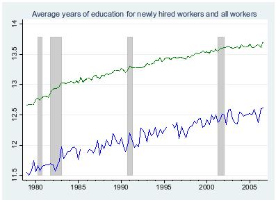
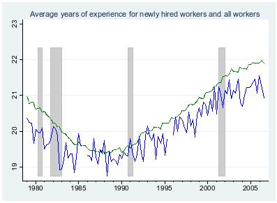
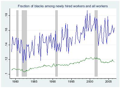
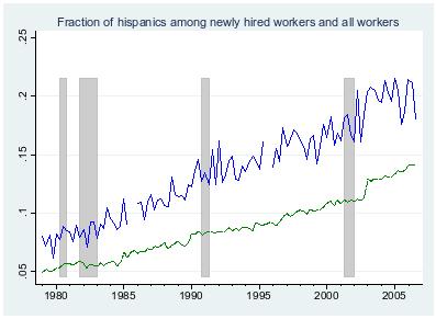
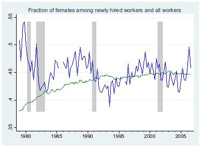
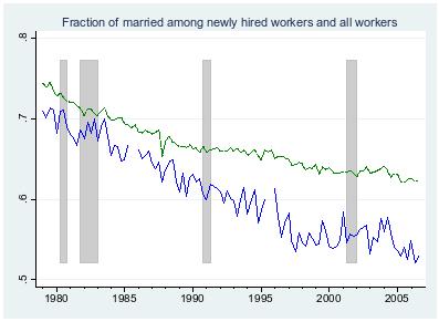
49 Figure 4: Characteristics of All and Newly Hired Workers Over Time. 48