MELT SPINNING OF CONTINUOUS FILAMENTS BY COLD AIR ATTENUATION

Transcription

1 MELT SPINNING OF CONTINUOUS FILAMENTS BY COLD AIR ATTENUATION A Thesis Presented to The Academic Faculty by Jun Jia In Partial Fulfillment of the Requirements for the Degree Doctor of Philosophy in the School of Materials Science and Engineering Georgia Institute of Technology December 2010

2 MELT SPINNING OF CONTINUOUS FILAMENTS BY COLD AIR ATTENUATION Approved by: Dr. Donggang Yao, Advisor School of Materials Science and Engineering Georgia Institute of Technology Dr. Karl Jacob School of Materials Science and Engineering Georgia Institute of Technology Dr. Youjiang Wang, Advisor School of Materials Science and Engineering Georgia Institute of Technology Dr. Wallace W. Carr School of Materials Science and Engineering Georgia Institute of Technology Dr. Kyriaki Kalaitzidou School of Mechanical Engineering Georgia Institute of Technology Date Approved: August 16, 2010

3 ACKNOWLEDGEMENTS I express my sincere thanks to my thesis advisors, Or. Donggang Yao and Dr. Youj iang Wang, for their invaluable guidance, support and encouragement during my PhD research. I would like to thank Dr. Karl Jacob, Dr. Wallace W. Carr and Dr. Kyriaki Kalaitzidou for serving in the thesis committee and providing valuable suggestions. I'm grateful to Dr. Wallace W. Carr's research group for allowing me to use their air drying system. I would like to thank Yaodong Liu, Xuxia Yao, Or. Kaur Jasmeet and Dr. Mihir Oka for helping with the fiber characterization experiments and their helpful advice. I wish to thank my former and current group members, Dr. Nagarajan Pratapkumar, Dr. Ruihua Li, Wei Zhang, Ram K.R.T., Sarang Deodhar, Ian Winters and Tom Wyatt, for their help and cooperation on experiments and valuable discussions. I would like to thank GTRI machine shop and ME machine shop for helping with the design and fabrication of the extrusion/fiber spinning dies. IV

4 TABLE OF CONTENTS ACKNOWLEDGEMENTS LIST OF TABLES LIST OF FIGURES SUMMARY iv x xi xviii CHAPTER 1 Introduction and Literature Review Fiber Spinning Technology Fundamental of Melt Spinning Tension in Melt Spinning Line Kinematics of Melt Spinning Formation of Fiber Structure Numerical Simulations Fundamental of Melt Blowing Crystallization Behavior of Isotactic Polypropylene Mesophase Structure Crystalline Structure Two Melting Endotherm Peaks Effect of Processing Temperature and Take-up Speed on Crystallinity in Melt Spinning Effect of Cooling Rate on Crystallinity 26 CHAPTER 2 Research Motivations and Objectives 27 v

5 CHAPTER 3 Design of Apparatus for Melt Spinning by Cold Air Attenuation Design of High Speed Air Jet Nozzle Incompressible Air Flow Compressible Air Flow Design of Spinneret Pack Experiment Setup 41 CHAPTER 4 Computational Fluid Dynamics Simulation of The Fiber Attenuation Model Description Material Properties and Viscosity Characterization Model Formulation Simulation Results and Discussion Velocity Profile and Distribution of Filament Polymer Viscosity Effect Processing Temperature Effect Air/Polymer Flow Ratio Effect Limitations 58 CHAPTER 5 Experimental Studies Materials Design of Parametric Studies Fiber Production 61 vi

6 5.4. Fiber Characterizations Fiber Microstructures Thermal Analysis Mechanical Properties Rheology Fiber Molecular Orientation Fiber Crystallization Behavior 68 CHAPTER 6 Experimental Results and Discussions Fiber Geometry Effect of Polypropylene Viscosity and Processing Temperature Effect of Air/polymer Volume Flow Ratio Fiber Morphology Fiber Molecular Orientation Crystallization Behavior of Resulting Fibers Crystallinity Crystal Form and Crystallite Size Fiber Mechanical Properties Melting and Crystallization Temperature Comparisons with Traditional Melt Spinning Fiber Properties 97 vii

7 Cost Analysis and Possibility of Scale up Fibers Made from Nylon 6 98 CHAPTER 7 Theoretical Analysis and Modeling of Cold Air Attenuation In Melt Spinning Process Introduction and Objectives Literature Review Model Formulation Model Description Governing Equations Constitutive Equations Boundary Conditions Method of Solution Validation of Computation Method Isothermal Model Effect of Model Geometry Length Effect of Polymer Viscosity Effect of Initial Fiber Velocity Effect of Air Flow Velocity Non-isothermal Model Modification of Calculation Method Effect of Processing Temperature 135 viii

8 Effect of Air Flow Speed Effect of Initial Fiber Velocity Comparisons Between Experimental Results and Model Simulation Results 140 CHAPTER 8 Conclusions and Suggestions for Future Studies Conclusions Suggestions for Future Studies 144 APPENDIX A Drawing of Spinneret Pack 147 A.1. Spinneret Die 147 A.2. Air Chamber 148 A.3. Air Nozzle 149 A.4. Insulation Piece 150 APPENDIX B Picture of Fiber Extruder 152 APPENDIX C Matlab Codes for Theoretical Modeling 154 C.1. Validation Model 154 C.2. Isothermal Model 154 C.3. Non-isothermal Model 155 References 159 ix

9 LIST OF TABLES Table 3-1 Air jet velocity comparisons. 31 Table 4-1 Materials properties of Polypropylene and air. 45 Table 5-1 First design of parametric studies on processing conditions. 60 Table 5-2 Second design of parametric studies on processing conditions. 62 Table 6-1 PP115 fiber diameters and their processing conditions. 71 Table 6-2 PP12 fiber diameters and their processing conditions. 72 Table 6-3 Crystallite size and 2θ value of 110 plane of PP115 fiber made at 220ºC. 87 Table 6-4 Melting and crystallization temperatures of resulting fibers. 92 Table 6-5 Fiber properties of fibers made by traditional melt spinning. 97 Table 6-6 Processing conditions and resulting fiber properties of Nylon-6 fibers. 101 Table 7-1Value of β and n from literature [44]. 109 Table 7-2 Material properties and processing conditions for the isothermal model with 5cm model geometry length. 125 Table 7-3 Material properties and processing conditions for non-isothermal case. 132 Table 7-4 Comparisons between experimental results and simulation results on final fiber diameter under various processing conditions. 141 x

10 LIST OF FIGURES Figure 1.1 A typical melt spinning setup. 2 Figure 1.2 Schematic of apparatus used for laser heating [8]. 3 Figure 1.3 Schematic diagram of melt spinning with liquid isothermal bath. (a) The normal LIB process; (b) The modified LIB process [19, 20]. 4 Figure 1.4 Illustration of the set-up used for the various types of spinline modification attempted: on-line zone cooling, on-line zone heating, on-line zone cooling and then heating [23]. 5 Figure 1.5 Schematic of dry-spinning process [24]. 6 Figure 1.6 Schematic of wet-spinning process [24]. 7 Figure 1.7 Detailed schematic of the melt blowing die: (a) sectional and (b) end-on view of the two pieces [29]. 8 Figure 1.8 Production line of nanofibrous materials [32]. 9 Figure 1.9 Cohesive fracture of a steady-state liquid jet [24]. 11 Figure 1.10 Break-up of a liquid jet due to capillary wave [24]. 11 Figure 1.11 The individual contributions to spinning line tension vs. distance from spinneret [24]. 12 Figure 1.12 The velocity profiles and gradient in (a) shear flow in a capillary, and (b) elongational flow in a spinline [51]. 13 Figure 1.13 Comparison of shear and elongational viscosity functions vs. shear and tensile stress of polypropylene [52]. 14 Figure 1.14 Variation of elongational viscosity with time at a constant elongational strain rate at 200ºC for polypropylene. Elongational strain rate (s -1 ): 0.6; 0.2; 0.05;Δ 0.02; 0.005; [53]. 15 Figure 1.15 Formation of fiber structure in melt spinning [54]. 15 Figure 1.16 Morphological models of polyethylene crystallization during melt spinning [55]. 17 Figure 3.1 Mechanism of Laval Nozzle. 33 Figure 3.2 Boundary conditions for simulation. 34 xi

11 Figure 3.3 Simulation results of static pressure, static temperature and Mach number. 35 Figure 3.4 Detailed schematic of the first design of cold air attenuation setup. 36 Figure 3.5 Detailed schematic of the second design of cold air attenuation setup. 37 Figure 3.6 Four different insulation plate designs. 38 Figure 3.7 Air flow velocity profile of in the air nozzle and with two different insulation plates shape. 40 Figure 3.8 Schematic of customized hydraulic piston-driven fiber extruder. 42 Figure 4.1 Model descriptions of geometry, sub-domains and boundary sets, where the SD1 and SD2 present polymer, while SD3 and SD4 present air. 44 Figure 4.2 Polypropylene viscosity dependence of shear rate at different temperature. 46 Figure 4.3 Polypropylene viscosity fitted by Cross law model at 180ºC. 47 Figure 4.4 Polypropylene viscosity fitted by Arrhenius law model. 48 Figure 4.5 DSC test of virgin polypropylene. 49 Figure 4.6 Temperature ramp with angular frequency at 1 rad/s for polypropylene. 49 Figure 4.7 The velocity profiles and gradient in a spinline. 52 Figure 4.8 Effect of polypropylene viscosity on fiber geometries, (a) low viscosity; (b) medium viscosity and (c) high viscosity. 53 Figure 4.9 Fiber geometries and temperature profiles at different processing temperature: (a) 200ºC; (b) 230ºC and (c) 260ºC. 55 Figure 4.10 Fiber geometries and temperature profiles at different air/polymer flow ratio: (a) low; (b) medium and (c) high. 57 Figure 5.1 Up: typical on-line ZZ polarized Raman spectra for polypropylene fibers with different draw ratios (A 1.5, B 2.5, C 3.0 and D 3.5); Bottom: Plot of draw ratio vs. the Raman intensity ratio and birefringence for the polypropylene fibers [94]. 67 Figure 6.1 Viscosity of PP115 at different temperatures and angular frequencies. 69 Figure 6.2 Viscosity of PP35 at different temperatures and angular frequencies. 70 Figure 6.3 Viscosity of PP12 at different temperatures and angular frequencies. 70 Figure 6.4 Fiber diameter of PP115 and PP12 made at 220ºC. 73 xii

12 Figure 6.5 Data fitting of the relation between fiber diameter and air/polymer volume flow ratio. 74 Figure 6.6 SEM photographs of fibers. 76 Figure 6.7 Typical ZZ polarized Raman spectra of PP115 fibers, compared with WXRD pattern. Fibers were made with different draw ratio at different temperatures (a) 1600 at 220ºC; (b) 330 at 220ºC; (c) 360 at 240ºC; (d) control (raw PP115 pellet). 78 Figure 6.8 PP115 fiber molecular orientation estimated by Raman spectra. 79 Figure 6.9 Crystallinity of resulting fibers made from PP 115 at different temperatures. 81 Figure 6.10 Crystallinity of resulting fibers made from PP 12 at different temperatures. 82 Figure 6.11 Wide-angle X-ray diffraction patterns of PP115 under various processing conditions. Inside the shaded box, the first number indicates the air/polymer flow ratio; the second one is the resulting fiber diameter. 85 Figure 6.12 WXRD spectra of typical PP115 fibers made at 220ºC. 86 Figure 6.13 Typical stress-strain curves of single filament. 87 Figure 6.14 Tensile strength of PP115 fibers. 89 Figure 6.15 Tensile modulus of PP115 fibers. 90 Figure 6.16 Tensile strength of PP12 fibers. 90 Figure 6.17 DSC heating thermograms of PP115 fibers with different endotherm peak shapes. 93 Figure 6.18 WXRD spectra patterns of fibers with one or two melting peek(s) in DSC. 94 Figure 6.19 DSC heating thermograms of PP115 fibers made with various heating rate. 95 Figure 6.20 DSC heating thermograms of cold drawn and original undrawn PP115 fibers. 96 Figure 6.21 Viscosity of Nylon-6 at different temperatures and angular frequencies. 98 Figure 6.22 Nylon-6 fiber diameter versus air/polymer flow ratio. 100 Figure 6.23 Polarized microscopy image of Nylon-6 fiber. 100 Figure 7.1 Nu vs. Re in cooling by forced convection of cylindrical body; ( ) data of Simmons; ( ) data of Mueller; ( ) data of Sano and Nishikawa; ( ) Kase and Matsuo s work [57]. 105 xiii

13 Figure 7.2 Comparison of the predictions of the 3D model with those of the 2D and 1D models [45]. 113 Figure 7.3 Schematic of the melt spinning process by cold air attenuation and the force balance on fibers. 115 Figure 7.4 Model description of geometry and boundary conditions of freely fall down fiber in Polyflow. 121 Figure 7.5 Polyflow simulation results for freely fall down fiber model with different model geometry in length, (a) 3 cm, (b) 4 cm, (c) 5 cm and (d) 10 cm. 123 Figure 7.6 Comparison between the results obtained by Polyflow and MATLAB for different initial geometry length, 3 cm, 4 cm, 5 cm and 10 cm. 124 Figure 7.7 Isothermal model: fiber diameter profiles with different stop point positions (Inset: magnified view). 127 Figure 7.8 Isothermal model: fiber diameter profiles with different polymer viscosity with air flow velocity at 100 m/s (Inset: magnified view). 128 Figure 7.9 Isothermal model: fiber diameter profiles with different polymer viscosity with air flow velocity at 20 m/s. 129 Figure 7.10 Isothermal model: fiber diameter profiles with different initial fiber velocity (Inset: magnified view). 130 Figure 7.11 Isothermal model: fiber velocity profiles with different initial fiber velocity. 130 Figure 7.12 Isothermal model: fiber diameter profiles with different air flow velocity. 131 Figure 7.13 Non-isothermal model: fiber diameter and temperature. 133 Figure 7.14 Non-isothermal model: fiber diameter and temperature with processing temperature at 240ºC and stop point position set at 5 cm. 135 Figure 7.15 Non-isothermal model: fiber diameter and temperature with processing temperature at 220ºC and stop point position set at 4.5 cm. 136 Figure 7.16 Non-isothermal model: fiber diameter and temperature with air velocity of 10 m/s and stop point position set at 7 cm. 137 Figure 7.17 Non-isothermal model: fiber diameter and temperature with air velocity of 35 m/s and stop point position set at 5 cm. 137 Figure 7.18 Non-isothermal model: fiber diameter and temperature with initial fiber velocity at 0.01 m/s and stop point position set at 9 cm. 139 xiv

14 LIST OF SYMBOLS AND ABBREVIATIONS h c Nu k a r π V f Q Re D V a ρ a Heat transfer coefficient Nusselt number Thermal conductivity of air Radius of fiber Circumference ratio Fiber velocity Polymer volume flow rate Reynolds number Air velocity Air density µ a Air viscosity ρ f C pf T f η η 0 T g C f cfm τ Polymer density Heat capacity of polymer Fiber temperature Polymer viscosity Polymer zero shear rate viscosity Fiber temperature Gravitational acceleration Air drag coefficient Cubit feet per minute Stress tensor xv

15 F ext F rheo F surf F aero F gray P xx P * A A * γ P M MFI n Mn PP Take up tension Rheological force Surface tension Aerodynamic force Gravity Tensile stress Fiber tensile strength Cross-section area at nozzle exit Cross-section area at nozzle throat Specific heat ratio Air pressure Mach number Melt flow index Birefringence Number average molecular weight Polypropylene PP115 Polypropylene with melt flow index of 115 PP35 Polypropylene with melt flow index of 35 PP12 Polypropylene with melt flow index of 12 ipp PA6 PA66 PLA PET LDPE Isotactic polypropylene Polyamide-6 Polyamide-66 Polylactic acid Polyethylene terephthalate Low density polyethylene xvi

16 SEM DSC DMA WXRD CFD FEM Scanning electron microscope Differential scanning calorimetry Dynamic mechanical analysis Wide angle X-ray diffraction Computational fluid dynamics Finite element method xvii

17 SUMMARY Melt spinning is the most convenient and economic method for polymer fiber manufacturing at industrial scales. In its standard setup, however, the thermomechanical history is often hard to control along the long spinline, resulting in poor controllability of the processing and fiber structure, and limited capability of producing very fine fibers. To address these process drawbacks, we developed and investigated an alternative melt spinning process where attenuation of continuous filaments is conducted solely by an annular high-speed cold air jet. This differs from the standard melt spinning process where filament stretching is driven by mechanical pulling force applied along the spinline. With the new process, the fiber is quenched by a symmetric cold air jet and simultaneously attenuated where an inverse parabolic velocity profile in molten fiber is expected. Since the formation of fiber structure is highly dependent on the process conditions, the new process will provide a unique and controllable operation window to study fiber attenuation and structural formation under high-speed cold air drawing. Assisted by computational analysis on air/polymer fluid dynamics, we designed a high speed jet attenuation spinneret pack consisted of an extrusion die, an isolation plate, an air chamber, and an air nozzle. We built a piston-driven melt extruder, mounted to a hydraulic press and retrofitted with a single orifice extrusion die and the above described spinneret pack. The diameter of the die orifice was 0.5 mm. Parametric experimental studies were carried out to investigate effects of process variables on resulting fiber properties, including fiber diameter, molecular orientation, crystallinity and mechanical properties. Theoretical modeling was conducted to analyze the non-isothermal fiber attenuation mechanism under cold air drawing conditions. xviii

18 Polypropylene was chosen as the polymer for the major part of the process study. The fibers produced by the new process showed a uniform diameter and a smooth surface appearance. The fiber diameter was found highly dependent on the polymer viscosity and processing conditions, including the processing temperature and the air/polymer flow ratio. The fiber diameter decreases with increasing of the air/polymer flow ratio and the processing temperature, and with decreasing of the polymer viscosity and the initial fiber velocity. Fibers with diameter of 7 µm were produced from the 0.5 mm diameter spinneret, yielding an equivalent drawing ratio exceeding 5,000. The molecular orientation of cold air attenuated fibers was found to increase with the increase of the air/polymer flow ratio. The maximum molecular orientation was observed at mild processing temperature ( ºC). The measured fiber mechanical properties, in general, correlated well with the molecular orientation. The tensile strength and modulus increased with increasing of the air/polymer flow rate. Although no post drawing and heat setting steps were performed, the single filament with diameter of 10µm (without post drawing) showed moderately good mechanical properties, with a tensile strength of 100 MPa and a modulus of 2.5 GPa. Orientation induced crystallization was found to be dominant in this new process. The fiber crystallinity increases with increase of the air/polymer flow ratio accompanied with formation of high molecular orientation. Low crystallinity fiber was associated with high processing temperature at relatively low air/polymer flow ratio. Only α-monoclinic crystalline was formed in the produced polypropylene fibers. For further demonstration, this process was also successfully applied to other polymer materials, including Nylon-6. xix

19 An isothermal Newtonian model was developed to analyze the single factor effect of processing conditions on fiber diameter. A non-isothermal model was implemented to predict the fiber diameter under different processing conditions. The predicted values compared favorably with the experimental data. The new knowledge obtained in this study would likely yield a new process for producing innovative fiber products. xx

20 CHAPTER 1 INTRODUCTION AND LITERATURE REVIEW 1.1. Fiber Spinning Technology The first man-made fiber, known as viscose rayon, was invented by French scientist and industrialist Hilaire de Chardonnet in Since then, synthetic fibers have been largely used in the textile industry for apparel applications and as reinforcement for composite plastics [1]. Compared with natural fibers, synthetic fibers can be produced inexpensively, easily and in large volume. Among all the synthetic fibers, polymer fibers are a major subset, which are usually made from polyesters, polyamides and polyolefins. Traditionally, polymer fibers are made by a spinning process, including melt spinning, dry spinning and wet spinning. During fiber spinning, a polymer melt or solution is usually extruded through a spinneret and taken up downstream by a winder to form a filament. In 1950s, a melt blowing process was developed to produce nonwoven fabrics that contain fibers finer than normal textile fibers [2]. The ultra-fine fibers in nonwoven fibers/fabrics made by melt blowing supersede traditional fibers in many highly demanding applications, such as filtration systems, super absorbents and medical fabrics. Recent developments in bi-component spinning and electrospinning processes paved new ways to produce finer fibers for wider applications, including biomedical applications such as tissue engineering scaffolds [3, 4]. Among all these methods, melt spinning and melt blowing are still the most convenient and economic methods of fiber manufacture because of their high productivity, not requiring the use of auxiliary materials and simplicity of the process. 1

21 In conventional melt spinning, a melted polymer stream is ejected into a gas, usually air at ambient temperature (Figure 1.1). The gas performs the main function of cooling the filament, and it exerts a drag force upon the rapidly moving filament. Inside the capillary die, the polymer melt experiences mainly shear flow, while outside of the die flow changes to uniaxial elongational flow. When the polymer melt is extruded from the spinneret, it exhibits a die swell phenomenon. Then under the drag force applied by the winder, fiber starts to attenuate and chain orientation and crystallinity take place within a short time before melt solidification by the air cooling effect. The comparatively simple and easy processing is the most important advantage of melt spinning. However, it also suffers from problems like fiber breakdown, variation in filament thickness, and limit to the fineness of fiber and spinneret clogging. Figure 1.1 A typical melt spinning setup. The mechanical properties of a filament can be improved by heat treatment of running filament in the spinline. For example, Suzuki et al. [5-18] developed a laserthinning method to produce microfiber by irradiating a carbon dioxide (CO 2 ) laser to fiber. One end of the zone-annealed fiber was connected to a jaw equipped with an 2

22 electric slider, whereas the other was attached to a slight weight. The zone-annealed fiber, moving downward at a speed of 500 mm/min, was heated by irradiating the CW CO 2 laser, and drawn instantaneously (Figure 1.2). The microfiber can be wound as a monofilament at winding speeds ranging from 100 to 2500 m/min. They have applied this method to PET, PA6, PP, PA66 and PLA fibers with diameter range of 1.5~5 µm. Various fiber properties were improved by this process, such as tensile modulus, tensile strength and birefringence. Figure 1.2 Schematic of apparatus used for laser heating [8]. A modified isothermal liquid bath was also used in melt spinning to produce high performance poly(ethylene terephthalate) fiber, reported by Cuculo et al. [19, 20]. In their experimental set-up (Figure 1.3), an isothermal liquid bath with temperature at 160ºC is placed under the spinning orifice with different distance to develop an extremely high level of tension in the threadline. With this modification, as-spun fibers with extremely high amorphous orientation and low crystallinity can be produced. The resulting fibers 3

23 show good mechanical properties which is similar to those made by commercial spindraw processes. (a) (b) Spinneret Spinneret Heated sleeve Heated sleeve L Cooling L Hot liquid jet LIB LIB Position L LIB0 30 cm LIB0 50 cm LIB0 100 cm LIB0 180 cm Liquid Spinline Take-up godet Liquid Spinline Take-up godet Figure 1.3 Schematic diagram of melt spinning with liquid isothermal bath. (a) The normal LIB process; (b) The modified LIB process [19, 20]. Some other efforts have been made to cool or quench filaments in the spinline to produce highly oriented amorphous yarn which is required for as-spun yarn to process into high tenacity yarn [21, 22]. In one of these methods, a liquid quenching medium is introduced. A highly oriented amorphous structure is formed by cooling the filaments in the spinline during high speed spinning. The effect of cooling bath position and temperature has been studied. Other than using a liquid quench bath, effect of modified air quenches on melt spinning process was also investigated [23]. As shown in Figure 1.4, a combination of enhanced and/or retarding air quenches is used to modify the threadline dynamics, resulting in significant improvement in spinning performance and as spun fiber 4

24 structure. With particular combination, produced fibers revealed high orientation and crystallinity, large crystal dimensions and greater mechanical properties. It was also claimed by the authors that this modified process can be applied to melt spinning over a wide range of take-up speeds. Cooling chamber positions ( cm) Range of heating chamber positions for OLZCH Spinneret Range of heating chamber positions for OLZH ( cm) Take-up Figure 1.4 Illustration of the set-up used for the various types of spinline modification attempted: on-line zone cooling, on-line zone heating, on-line zone cooling and then heating [23]. Solution spinning is another method to make fiber if a suitable solvent can be found. Solution spinning can be classified primarily into two methods, dry spinning and wet spinning. The typical solution spinning processes are shown in Figure 1.5 and Figure 1.6. In dry spinning, the filament is formed by the evaporation of polymer solvent into air or an inert gas phase. The wet spinning is where a solution of a polymer is spun through a 5

25 spinneret into a liquid which can coagulate the polymer. It can be further divided into three methods: the liquid-crystal method, the gel method and the phase-separation method. In the liquid-crystal method, a liquid-crystalline solution of a lyotropic polymer is solidified through the formation of a solid crystalline region in the solution. In the gel method, polymer solution is solidified through the formation of intermolecular bonds in the solution. In the case of phase separation, two different phases appear in the solution, one polymer-rich, and the other polymer-lean. However, the solution spinning process is too complicated and it is difficult to find the proper solvent for every polymer. Therefore, this method can only be applied for limit types of polymers to produce fibers, particularly when melt spinning is not a feasible process for these polymers. 1, metering pump; 2, spinneret; 3, spinning line; 4, drying tower; 5, 6, 7, take-up elements; 8 and 9, inlet and outlet of the drying gas. Figure 1.5 Schematic of dry-spinning process [24]. 6

26 1, inlet of the spinning dope; 2, spinneret; 3, spinning line; 4, spinning bath; 5, take-up godet; 6, 7, inlet and outlet of the spinning bath; 8, plasticizing bath; 9, 10, drawing elements. Figure 1.6 Schematic of wet-spinning process [24]. For many years, melt blowing has been used for producing microfibers of finite length [25, 26]. In conventional melt spinning, a polymer stream is ejected into air at ambient temperature and pressure. However, the gas performs a very different task in melt blowing. A common feature for different melt blowing processes is that, in addition to spinning orifices, hot air nozzles are placed in the vicinity to draw the threads. Once mixed with the colder ambient air, there is simultaneous cooling and solidification and often the thread breaks. The original work on melt blowing dates back to the efforts of Naval Research Laboratory in the 1950s. Wente [2] first described the construction of a melt blowing die composed of a number of orifices and slots. Motivation for his work was to make the subdenier fibers for filters on drone aircraft. Based on the slot concept and an extension of sheet die technology, Exxon was able to improve Wente s work to a commercial production scale [27, 28]. Since then, a number of companies have used the technology to produce commercial nonwoven products. In general, these commercial products are composed of fibers with average diameters about 1-2 µm. 7

27 Figure 1.7 Detailed schematic of the melt blowing die: (a) sectional and (b) end-on view of the two pieces [29]. The limitations of melt blowing include the stochastic process dynamics, the high energy consumption and the very short length of the fiber produced. If the melt blowing technology can be extended to submicron fiber size, it would provide a much easier, faster, and cheaper alternative to ultra fine fiber industry. Hence, the major focus of melt blowing research is to extend the technology to nanofibers [29-31]. Poly(butylene terephthalate), polypropylene, and polystyrene nanofibers with average diameters less than 500 nm have been produced by Ellison et al. [29] using a single orifice melt blowing apparatus (Figure 1.7) and commercially viable processing conditions. Furthermore, analysis of fiber diameter distributions reveals they are well described by a log-normal distribution function regardless of average fiber diameter, indicating that the underlying fiber attenuation mechanisms are retained even when producing nanofibers. Fiber breakup was observed under certain processing conditions, which was believed driven by 8

28 surface tension and these instabilities may represent the onset of an underlying fundamental limit to the process. Podgorski et al. [32] developed a modified melt-blown technology, which facilitated the production of filters composed of micrometer as well as nanometer sized fibers. The schematic of the set up for obtaining fibers by blowing a melted polymer and details of the die construction are shown in Figure 1.8 (a polymer stream is denoted there by 1 and the air stream by 2). The processing conditions and the die orifice diameter were not reported. Figure 1.8 Production line of nanofibrous materials [32]. The research group in University of Oklahoma conducted a series of studies on melt blowing process, including the effect of die shape on air flow profile, filament motion and CFD simulation [26, 33-50]. A sharp and a blunt die are designed and studied in their paper. The results show that the blunt die is a better option to reduce turbulence fluctuation along the path of the polymer fiber. In summary, melt blowing is typically used to produce nonwoven fabrics and usually the fiber strength is low. To make continuous filaments, melt spinning and solution spinning are the two major processes. Since solvent is introduced to dissolve the polymer, 9

29 solution spinning requires a relative complicated manufacturing set up and limits its application in industry. Therefore, the melt spinning process draws lots of interests in research to improve the fiber properties by modifying the spinline thermal and mechanical conditions as indicated in the literature. The mechanisms of how the processing conditions affect fiber properties will be discussed in the next sections Fundamental of Melt Spinning Tension in Melt Spinning Line Fiber breakage is the major issue in melt spinning. The physical mechanisms of the fiber breakage can be explained by two types of processes, cohesive failure and capillary wave breakage. In the first process, rapture occurs when the tensile stress in a polymer fiber exceeds some critical limit, the tensile strength. As shown in Figure 1.9, from the spinneret, initially the tensile stress (P xx ) is lower than the fiber tensile strength (P * ). Downstream along the spinline, both the tensile stress and fiber strength increase, but the tensile stress increases much faster than the tensile strength. At some critical point, the tensile stress will exceed the fiber tensile strength, thus resulting in fiber breakage. The second process, capillary wave breakage, is associated with surface tension. As shown in Figure 1.10, a polymer melt splits into individual drops when the growing amplitude of the capillary waves reaches the radius of the undistorted jet. 10

30 Figure 1.9 Cohesive fracture of a steady-state liquid jet [24]. Figure 1.10 Break-up of a liquid jet due to capillary wave [24]. Integration of the momentum conservation equation yields the following equation of force balance at a distance x from the spinneret: F + F ( x) = F ( x) + F ( x) + F ( x) + F ( x). (1) ext grav rheo in surf aero F ext, F grav, F rheo, F surf, F in and F aero represent take-up tension, gravity, rheological force, surface tension, inertia and aerodynamic force. Figure 1.11 illustrates the distribution of 11

31 individual force contributions along the spinline of a Nylon 6 monofilament [24]. Compared with other forces, the surface tension can be neglected as being less than 1% of the take up tension. Gravity and inertia provide an appreciable effect on the filament tension near the spinneret and then keep decreasing downstream the spinline. Aerodynamic and rheological forces are the major forces balancing with take up tension along the spinline. The take up tension is assumed to be constant along the spinline in normal spinning speed. At higher spinning speed, the aerodynamic force plays a dominant role thus the assumption of constant force along the spinline is not valid. Figure 1.11 The individual contributions to spinning line tension vs. distance from spinneret [24] Kinematics of Melt Spinning The velocity distribution and profile of the polymer melt appear in different forms along the spinline, which play an important role in the fiber formation. Inside the spinneret channel, the polymer flow is a typical Poiseuille flow with a parabolic velocity 12

32 profile. By assuming an incompressible Newtonian liquid of viscosity η through a capillary of radius R and length L, the radial velocity distribution can be described as: P 2 2 V ( r) = ( R r ), (2) 4η L where P is the pressure difference between the inlet and outlet of capillary. Figure 1.12 The velocity profiles and gradient in (a) shear flow in a capillary, and (b) elongational flow in a spinline [51]. When polymer is extruded out the orifice, a phenomenon of die swell is observed due to the relaxation of stored elastic energy. The degree of swelling depends on the conditions of extrusion, temperature and geometry of the die. For example, in melt spinning, the die swell ratio decreases with the increase of extrusion temperature. Under take up tension, the flow of polymer melt transits from shear flow to elongational flow, or uniaxial extensional flow. In elongational flow, the velocity keeps increasing along the spinline and finally reaches the take-up speed. Figure 1.12 shows the differences on velocity profile between shear flow and elongational flow. 13

33 Figure 1.13 Comparison of shear and elongational viscosity functions vs. shear and tensile stress of polypropylene [52]. The fiber formation occurring underneath the spinneret is affected by elongational viscosity η* over a wide range of temperatures. In a steady state elongation, the elongation viscosity η* is nearly constant and equal to 3-times Newtonian viscosity η 0 (the so-called Trouton s viscosity model) in the range of moderate elongation rate: * η = 3η 0. (3) When the elongational rate exceeds some critical value, the elongational viscosity deviates from the 3η 0 model for a Newtonian liquid because of the dominating elastic deformation. The typical shape of the elongational viscosity as a function of tensile stress for polypropylene melts is shown in Figure For small stress, the elongational viscosity fits the threefold value of shear viscosity. When the stress increases, the shear viscosity decreases more abruptly than the elongational viscosity. In highly viscoelastic materials such as molten polypropylene, steady state elongational flow is not possible at higher elongational rate because the rapid increase of tensile stress is followed by cohesive fracture. Figure 1.14 shows the time dependent 14

34 elongational viscosity of polypropylene. At low elongational rate, the elongational viscosity increasess smoothly and finally reaches the constant value 3ηη 0. For higher elongational rate, the elongational viscosity increases dramatically once beyond the critical time. The critical time also decreases with increasing elongational rate. Figure 1.14 Variation of elongational viscosity with time at a constant elongational strain rate at 200ºC for polypropylene. Elongational strain rate ( 0.005; [53]. (s -1 1 ): 0.6; 0.2; 0.05; ; 0.02; Formation of Fiber Structure Figure 1.15 Formation of fiber structure in melt spinning [54]. 15

35 Formation of molecular orientation and crystalline plays an important role in melt spinning and thus affects the ultimate structure and physical properties of fibers. Figure 1.15 describes a typical fiber structure formation process in melt spinning. Molecular orientation arises from parallelization of the molecular chains along the fiber axis in both the crystalline and non-crystalline regions. During melt spinning, the molecular orientation develops in two stages: in spinneret channel and under elongation. Molecular alignment is developed when the polymer melt is forced through a capillary channel. As it comes out of the spinneret, the molecular alignment becomes disorientated and thus contributes very little to the final fiber orientation. The major contribution of orientation is made by the elongational flow along the spinline. The parallel velocity gradient, the relaxation time distribution and the elapsed time are the important factors which affect the molecular orientation. For example, a higher heat transfer coefficient results in an increase in orientation since it causes more effective freezing of orientation on filament quenching. The molecular orientation also increases with the increase in takeup speed, extrudate viscosity and reciprocal of polymer mass flow rate. 16

36 Figure 1.16 Morphological models of polyethylene crystallization during melt spinning [55]. Non-isothermal and oriented crystallization of the filament is also developed during melt spinning, and the oriented crystallization plays a privileged role in fiber formation. It was observed by Keller [56] that during elongation, the nuclei are formed along the spinline in the form of platelets known as row nucleation. With the increase of take-up speed, the morphological forms of crystallization alter from spherulitic to row nucleated twisted lamellae, and finally to row nucleated lamellae untwisted. A morphological model of melt spun PE proposed by Dees and Spruiell [55] is shown in Figure The crystallization is also very sensitive to the spinning conditions. In contrast to orientation, crystallinity decreases with the increase of heat transfer coefficient and increases with the increase of fiber diameter since slow cooling gives more time for molecules to crystallize. 17

37 Numerical Simulations Since the early 1960s a number of researchers have started to analyze the dynamics of melt spinning by establishing a set of simultaneous partial differential equations over a wide range of spinning conditions. Kase et al [57, 58] studied the axial and radial variations in temperature and velocity of steady spinline, and stability of unsteady spinline using multi-part study. A 3-D axisymmetric temperature profile in a constant radius fiber has been solved by Morrison in 1969 [59]. Moutsoglou [60] studied the temperature field subjected to an exponential stretching rate. The numerical analyses of melt spinning were also extended from isothermal Newtonian flow to viscoelastic fluid, nonisothermal Newtonian flow, nonisothermal viscoelastic flow and recently flow with crystallization [61-64] Fundamental of Melt Blowing Melt blowing is a one step process for producing nonwoven fabrics from polymer melt with high speed hot air attenuation. The microfibers made by melt blowing usually have diameters in the range of 2 to 4 µm with very short length. The basic product properties include random fiber orientation, web strength, fiber diameter and filtration characteristics. Most of the efforts in this area focused on optimization of process conditions for improving those product properties [38, 65-69]. Unlike the melt spinning process, fundamental studies of melt blowing are seldom reported except some numerical modeling studies. The interest in the development of a numerical model for the melt blowing process dates back to 1990s. Uyttendaele and Shambaugh [70] developed a 1-D model by assuming fiber motion only in the axial direction. Their model can successfully predict the fiber attenuation under the action of the hot air steam within relatively low 18

38 spinning speeds. Rao and Shambaugh [71] expanded the 1-D model to a 2-D model in which the fiber motion is considered in a plane. Recently, a 3-D model involving the simultaneous solution of the momentum, energy and continuity equations has been developed by Marla and Shambaugh [45]. Other relevant numerical models of melt blowing have also been investigated by a number of researchers, such as simulation of the fiber movement, air-jet flow field and air drawing [39, 40, 72]. Details on these numerical models will be discussed later Crystallization Behavior of Isotactic Polypropylene Isotactic polypropylene (ipp) is a widely used polymer material in the fiber industry because of its ease of processing, low cost and rapid crystallization. The crystallization process of ipp is complicated, sensitive to the processing conditions. A less ordered mesophase can be formed at high cooling rate and low orientation. The crystalline structure usually results from low cooling rate and modest to high orientation Mesophase Structure Boye et al. [73] reported a smectic structure observed on a melt-extruded isotactic polypropylene quenched in ice water. The sample density was g/ml which is higher than the amorphous polypropylene. In addition, two broad peaks located at 2θ=14.8º and 21.3º were exhibited in the X-ray diffraction spectra. Choi and White [74] studied the effect of cooling rate and spinline stress on the formation of different crystalline forms. The sample filaments were prepared by melt spinning at various melt temperatures and take-up speeds. The filaments were quenched by either ice water or ambient air before taken up by roller. Smectic structures were only detected on the filaments quenched by ice water. It was also observed that the smectic 19

39 structure transits to α-monoclinic crystalline structure with increasing of draw-down ratio and spinline stress at melt temperature 200ºC and 230ºC. However, this transition was not observed when melt temperature increased to 260ºC. They also developed continuous cooling transformation (CCT) curves and a map of crystalline form as a function of cooling rate and spinline stress. The CCT curves and the map were then used to predict the formation of cross-sectional variation structure in thick filaments and rods. Gorga et al. [75] studied the meso-to-α phase transition in ipp made from quenching and melt spinning for two different polypropylene (ipp E and ipp S ) with similar molecular weight profile. The ipp S melt spun fibers showed mesophase structure when the take up speed is in the regime of m/min. This range changed to m/min for ipp E for the formation of mesophase. When the take-up speed exceeds 1500 m/min, the α- monoclinic structure was redeveloped for both ipp E and ipp S melt spun fibers. The mesophase structure was also observed in the non-oriented ipp E sample quenched by icewater. However, the mesophase was not formed for ipp S even when it was quenched by liquid nitrogen, the hardest quenching conditions used in their study. It was indicated that the molecular orientation increases with increasing take-up speed for all crystalline, mesophase and amorphous structures. Mechanical properties showed strong relation with molecular orientation, but it is unrelated with the presence of mesophase Crystalline Structure The crystalline phase of isotactic polypropylene has three kinds of crystalline forms: α-monoclinic, β-hexagonal and γ-triclinic. ipp predominately crystallize in α-monoclinic under usual conditions. For example, ipp fibers made by melt spinning usually exhibits α-monoclinic crystalline structure. The β-hexagonal and γ-triclinic crystalline can be 20

40 formed under extreme conditions or by introducing nucleating agents. The three different crystal forms can be characterized by X-ray diffraction method. For α-monoclinic, it shows three strong reflections located at 2θ=14.2º, 17.1º and 18.6º which correspond to 110, 040 and 130 plane respectively. β-hexagonal has a strong peak in X-ray diffraction spectra located at 2θ=16.1º which represents 300 plane. For γ-triclinic, the 100, 040 and 130 planes show strong reflection at 2θ=13.9º, 16.8º and 20.1º. Broda [76] observed the formation of β-hexagonal crystal in ipp fibers made by melt spinning with the addition of quinacridone pigment. In this paper, the crystallization behavior was compared for colored and noncolored fibers melt spun under various conditions. In noncolored fibers, the mesophase was observed for modest take-up velocity and α-monoclinic was formed at low or high take-up velocity. The content of mesophase was found increased at higher melt temperature because of low orientation and high cooling rate. In colored fibers, the β-hexagonal was observed at low take-up velocity for both low and high melt temperature. When the take-up velocity increases, the content of β-hexagonal crystalline became smaller and finally transited to a crystalline structure with only α-monoclinic. This transition was explained by the marginal nucleating effect of the pigment at high take-up velocity where the crystallization is governed by the orientation. Al-Raheil et al. [77, 78] studied the spherulitic structure of isotactic polypropylene from melt by polarized light and SEM. Their results showed that α and β spherulitic can be obtained for crystallization from melt below 132ºC. Above 132ºC, only α type spherulitic was observed for isothermal crystallization. Their study also indicated that α spherulitic has a more complicated crosshatched lamellar structure than β spherulitic. 21

41 γ-triclinic crystalline structure is very difficult to form under normal conditions. Wittmann and Lotz [79] reported the formation of γ-phase crystal obtained from low molecular weight extracts of pyrolyzed ipp crystallized from melt. Several major differences from α-phase crystal were claimed in their study. The γ-phase crystal elongates along the b*-axis direction with chain axis inclined at 50º to the lamellar surface. And the screw dislocations were found for γ-phase crystal. Shen and Li [80] studied the β- and γ-form distributions of ipp injection molding controlled by melt vibration. The β-form crystals were obtained in injection-molded ipp by either conventional injection molding or vibration assisted injection molding. The content of β- form crystals can be controlled by applying different vibration modes. The γ-form crystals can only be obtained under relatively low vibration frequency and large vibration pressure amplitude Two Melting Endotherm Peaks It was reported that sometimes isotactic polypropylene has two melting endotherms in its DSC thermograms. Different theories have been proposed to explain this melting behavior, such as formation of two different crystal structure and crystalline size, recrystallization and reorganization during the heating in DSC scan. Somani et al. [81] studied the orientation-induced crystallization in ipp melt by shear deformation. The DSC thermograms of sheared ipp samples showed two melting peaks: one at 164ºC and the other at 179ºC. Further investigations suggested that the first peak corresponds to the nominal melting of the unoriented spherulites consisting of folded chain crystal lamellae. And the second one is from the melting of oriented crystalline structures. 22

42 Yan and Jiang [82] investigated the effect of drawing condition on the observed properties of drawn, compression-molded isotactic polypropylene. The ipp pellets were firstly melted and compression-molded to sheets at 195ºC. The sheets were then cooled naturally under pressure. An Instron tensile testing machine was used to draw the sheet under various temperatures and draw ratios. For the sample with high draw ratio and high heating rate used in DSC, it was observed two melting endothermic peaks in DSC thermograms. The position of the two melting peaks was found influenced by drawing conditions. The peak at lower temperature is related to the drawing ratio and temperature, while the peak at higher temperature only depends on the draw ratio. All the tested samples exhibited typical α-form crystalline in X-ray diffraction pattern. They assumed that the peak at lower temperature comes from extremely thin quasi-amorphous or crystalline layers among neighboring microfibrils, whereas the peak at higher temperature comes from the lamellar crystals within microfibrils. Kim et al. [83] conducted a study on melting of isotactic polypropylene isothermally crystallized at different temperatures. Double melting peaks were observed for crystallization temperature in the range of 110ºC to 140ºC. The double melting peaks are contributed from two preexisting crystal fractions with different T m. Pae and Sauer [84] studied the effects of thermal history on isotactic polypropylene. A double endothermic peak was observed after a series of stepwise annealing treatments when the final annealing temperature is close to 160ºC. Jain and Yadav [85] studied the melting behavior of isotactic polypropylene isothermally crystallized from melt. The development of the multiple fusion endotherms was investigated based on different crystallization temperature. The crystal imperfections 23

43 play an important role with crystallization temperature at or lower than 127ºC. Under heating, the crystallized fraction recrystallized to a fraction with higher degree of perfection which has higher melting temperature. When the crystallization temperature increases, the crystallization rate decreases. The higher melting peak starts to disappear and finally merges with the lower melting peak to a single peak at T c =127ºC. At crystallization temperature higher than 127ºC, the multiple peaks were attributed to the existence of different crystalline species with different crystal disorder and stereo-block character. Qudah et al. [78] also observed double melting peaks on DSC curves when the isotactic polypropylene crystallized isothermally above 132ºC at which only α- monoclinic crystalline was formed. It was concluded that the peak at low temperature comes from the melting of crosshatched lamellae of α-monoclinic crystalline, while the other peak is related to melting of the radial and the reorganized tangential lamellae. Guerra [86] discovered two different modifications of α-monoclinic crystalline by annealing which has difference in order. The recrystallization from less ordered modifications to more ordered ones results in a large increase of melting temperature which leads to the double peak of melting endotherm. Aboulfaraj et al. [86] observed double peaks in melting endotherm for a thick plate of isotactic polypropylene. The appearance of double melting peaks was attributed to the formation of different crystal forms, α-monoclinic and β-hexagonal phases. A distribution of α and β crystal forms was developed by a slow solidification process. The α form crystal was found dominant on the surface and coexisted with β form crystal inside the 24

44 plate. The portion of β form crystal changes from 0 to 60% from the surface to the core of the sample plate Effect of Processing Temperature and Take-up Speed on Crystallinity in Melt Spinning As summarized in the previous part, the crystallization of polymer during melt spinning is a complex process which is governed by many competing factors. It was reported by Cao et al. [87] that the polypropylene crystallization behavior is influenced by two main competing factors, cooling rate and crystallization rate. In their studies, two kinds of polypropylene with different melt index values were used to produce fibers by melt spinning process. The experiments were conducted at different temperatures with various take-up velocities. The fiber crystallinity was characterized in terms of density and the relation between fiber crystallinity and take-up velocity was studied. At high processing temperature (270ºC and 290ºC), the crystallinity firstly decreases and then increases with the increase of take-up speed. However, at low processing temperature (210ºC and 250ºC), the crystallinity keeps constant which does not change with the takeup velocity. This phenomenon was explained by the concept of competitive effect of cooling rate and crystallization rate. Both the cooling rate and crystallization rate increase with the increase in take-up velocity. At low take-up velocity, the cooling rate dominates the crystallization process since the spinline stress is low. Therefore, the crystallinity decreases with increasing take-up velocity. However, when take-up velocity increases to some point, the crystallization rate becomes dominant in the crystallization process due to the increasing spinline stress and high orientation. Consequently, the fiber crystallinity starts to increase with increasing take-up speed. 25

45 Effect of Cooling Rate on Crystallinity Crystallization of polymer under varied processing conditions is a very complicated process and cannot to be described by any single-valued effect, because it is not possible to separate the thermodynamics from kinetics effects during the process. Piccarolo et al. [88] developed a specially designed experimental setup which can independently study the effect of cooling rate on polymer crystallization. The cooling rate covers an overall variation from ºC/s. It can be controlled by changing the coolant, flow rate, temperature, or the sample thickness. The crystallization behavior of ipp, PET and PA6 were studied. The crystallinity was characterized in terms of density. A dramatic decrease in ipp density was found when the cooling rate reaches about 100ºC/s. This critical cooling rate decreases to 10ºC/s and 2ºC/s for PA6 and PET respectively. After the critical point, the polymer density remains almost at a constant value depending on the final phase structure. A mesophase to α-monoclinic phase transition was observed in ipp samples when the cooling rate is above 100ºC/s. 26

46 CHAPTER 2 RESEARCH MOTIVATIONS AND OBJECTIVES Melt spinning is the most convenient and economic method for polymer fiber manufacturing at industrial scales. In its standard setup, melt spinning involves mechanical stretching of polymer filaments both in a liquid and in a solid state. However, this process is subjected to some inherent process flaws. Particularly, the process is operated in a relatively narrow process window, mainly designed for stretching the filament with a constant tensile force and cooling the filament using cross air flow. Because a constant tension is applied during fiber extenuation, the tensile stress rapidly increases along the spinning line. This can cause instabilities and difficulty in producing fine fibers. More importantly, the thermomechanical history is often hard to control in this narrow process window, resulting in poor controllability of the process and the fiber structure. As discussed in the literature review, some efforts have been made in modifying the spinline thermal and mechanical dynamics to improve fiber properties or produce finer fibers. One approach is to heat the spinline by hot air or laser, such as melt blowing and melt spinning with online laser heating. With the increase of spinline temperature, the filaments tend to be attenuated more and usually finer fibers can be achieved. However, the fibers created from melt blowing are typically discontinuous with short fiber length. The online laser heating process also needs specially designed equipment and post drawing process to achieve high fiber strength. Another approach is to apply a liquid bath on the spinline to increase the spinline stress and control the filament temperature. With 27

47 this modification, highly orientated highly crystalline fibers or highly orientated amorphous fibers can be obtained dependent on the liquid bath conditions. However, the complex setup and processing procedure make it impossible for massive industry production. Therefore, it is highly desirable to develop a new process to produce continuous filaments with modified spinline thermal and mechanical environment. In addition, this process should satisfy the requirements of industrial production, such as easy setup, stable process, environmental friendliness, solvent free process, and mass productivity. To achieve these purposes, we investigated and developed a modified melt spinning process with an annular high-speed jet nozzle to produce continuous polypropylene filaments by cold air drawing only. With this setup, the fiber emerged out of the die orifice is quenched and simultaneously attenuated by a symmetric cold air jet. Since the formation of fiber structure is highly dependent on the processing conditions, the new process will provide a unique operation window to study fiber attenuation and structural formation under high-speed cold air drawing. The new knowledge obtained in this study would likely yield a new process for producing innovative fiber products. With these motivations, the specific objectives of the project are to: Design and build a high speed air jet nozzle. Retrofit a melt-spinning unit with a specially designed spinneret and high speed air nozzle. Study the non-isothermal fiber attenuation mechanisms by computational fluid dynamics method. Based on the simulation results, perform a parametric study under different process conditions which include processing temperature, air velocity and 28

48 polymer volume flow rate. Investigate the relationships between the process conditions and resulting fiber properties, such as fiber geometry, orientation, crystallization, thermal and mechanical properties. Build a mathematical model to theoretically study the fiber attenuation mechanisms, mainly on how the resulting fiber geometry is affected by the polymer melt temperature, the polymer/air throughput ratio, and the polymer viscosity. Also use this model to predict the final fiber diameter. 29

49 CHAPTER 3 DESIGN OF APPARATUS FOR MELT SPINNING BY COLD AIR ATTENUATION An annular single orifice melt spinning equipment at laboratory scale was assembled to produce the microfiber by high speed air jet attenuation. This kind of design has several notable advantages in fundamental process study compared with commercial multi-port extrusion die. Firstly, non uniform polymer distribution problems can be avoided and more uniform fibers can be produced in the single orifice design. Secondly, without the interference from other orifices, it is easier to control the operation conditions and to collect or take up the produced single continues filaments. A high speed air jet nozzle was attached underneath the spinneret to generate a parallel high speed air jet to elongate the melt polymer once it was extruded out of the orifice. Since cold air was used, an insulation piece made from Teflon was inserted between the hot die and the cold air chamber to prevent the spinneret die from cooling. A winder was used to collect the produced fiber without applying any tension on the fiber threadline. The detail of this design is discussed in later part of this chapter Design of High Speed Air Jet Nozzle A convergent and divergent nozzle was designed and used to generate high speed air flow. When the stagnation pressure is close to atmospheric pressure, the air is considered incompressible and the air flow field is directly converted from flow rate measured by flow rate meter. When the air pressure is much higher than atmospheric pressure, the air 30

50 is then considered as compressible and a supersonic air flow may be generated under certain conditions based on the nozzle geometry Incompressible Air Flow The velocity of the air jet at the exit plane of the nozzle can be calculated in terms of volume flow rate and nozzle cross-sectional area when the gas pressure is close to the atmospheric pressure. The air density is assumed to be constant in this case. The volume flow rate is the same anywhere in air flow line, which means the volume flow rate measured at the testing position is the same as that at the exit plane of nozzle. Hence, the air velocity can be calculated by the following equation: V = Q / A (4) a where A is the nozzle cross-sectional area, V a is the air jet velocity, and Q a is the volume flow rate of air jet. To validate the calculated air velocity, a manometer was used to measure the air velocity at the nozzle exit plane. The calculated and measured air velocities obtained at different volume flow rates are listed and compared in Table 3-1. Table 3-1 Air jet velocity comparisons. Air Volume Flow Rate (CFM) Calculated Velocity (m/s) Measured Velocity (m/s) a The difference between the calculated and measured velocities might result from the assumption of a constant air density, since the air density will deviate from assumed constant value once the air pressure increases to a relative high value at high flow rate. 31

51 Compressible Air Flow The convergent and divergent nozzle is also called Laval nozzle, named after Gustaf de Laval, a Swedish inventor. Laval nozzles were widely used in numerous industrial applications, e.g., steam turbines, rocket engines, mixing devices, thermal spraying facilities, etc [41, 45, 46, 89-91]. The gas flow through a Laval nozzle can be accelerated to a supersonic flow. The working mechanism can be explained from the basic continuity and momentum equations of compressible gas flow [92]: dv d ρ da 0 = + + (5) V ρ A 2 dp V 0 = + d ρ 2 (6) where A is the cross-sectional area, V is the gas velocity, ρ is the density, and p is pressure. By introducing 2 a = dp d ρ and M = V a (Mach number), a relation between the infinitesimal area element, da, and the infinitesimal velocity change, dv, can be obtained from Equations (5) and (6): da dv 2 = ( 1 M ) (7) A V Therefore, if a nozzle is composed of a converging nozzle first and then the diverging nozzle, the velocity of the gas flowing through it can be continuously increased in the direction of flow from subsonic to supersonic, as shown in Figure

52 M<1 V increase V increase M>1 da<0 P decrease P decrease da>0 Figure 3.1 Mechanism of Laval Nozzle. The following equations are the property ratios for the steady, isentropic and onedimensional flow of a perfect gas, which are derived from the basic governing equations. T T 0 γ 1 2 = 1+ M (8) 2 p p 0 γ 1 = 1+ 2 M ρ0 γ 1 = 1+ ρ 2 M 2 2 γ ( γ 1) ( γ ) 1 1 (9) (10) A * A 1 2 γ 1 2 = 1 M M + γ ( γ + 1) 2( γ 1) (11) where P * A and A are the cross-sectional areas at the throat and the exit, respectively, and γ = C C is the specific heat ratio. V To reach a supersonic speed, the nozzle needs to operate under an appropriate condition at which the above-defined ratios strictly obey Equations (8)-(11). The initial conditions were calculated by assuming that the air flow inside the nozzle is an isentropic flow of a perfect gas. With a cross-sectional area ratio of 1.08 between the outlet and the throat, the Mach number was calculated to be The pressure and temperature ratios were then determined, using this Mach number, to be 0.35 and 0.74, respectively. With these nozzle design parameters, the outlet air pressure was expected to be identical to the back pressure, i.e., atmospheric pressure in our case. Thus the inlet pressure should be set 33

53 to 42 psi (289.6 KPa) with p p 0 =0.35 and p =14.7 psi (101.3 KPa). The air temperature at the exit was calculated to be 222 K with an initial temperature of T 0 =300 K at the inlet. inlet: P 0 =42 psi T 0 =300 K wall centerline outlet: P=14.7 psi Figure 3.2 Boundary conditions for simulation. CFD simulations were conducted using Fluent to analyze the air flow in the Laval nozzle and optimize our nozzle geometry. The axisymmetric nozzle geometry was imported to Fluent with the boundary conditions as shown in Figure 3.2. To reduce the difficulty and cost of making the nozzle, we modified the profile of the divergent part to a straight line. A testing case with the following setting of parameters was simulated to investigate the effect of the nozzle geometry on the air flow. An ideal gas and an inviscid flow model were used. The air pressure and temperature at the inlet were 42 psi and 300 K, respectively, and the exit air pressure was set to atmospheric pressure. Figure 3.3 shows the simulation results based on one geometrical design, including static pressure, static temperature and Mach number. Along the air flow direction, the air pressure kept decreasing to atmospheric pressure, the air temperature kept decreasing, and the air flow speed continuously increased to a Mach number of These simulation results verified our calculation results from the equations, and a Laval nozzle made of metal was fabricated according to this geometry. 34

54 (a) Absolute pressure (psi) (b) Static temperature (K) (c) Mach number Figure 3.3 Simulation results of static pressure, static temperature and Mach number. 35

55 3.2. Design of Spinneret Pack Based on the simulation results, a cold air attenuation spinneret pack was designed which is consisted of an extrusion die, an insulation plate, an air chamber, and an air nozzle. In the first design, as shown in Figure 3.4, the compressed cold air went into the nozzle through multiple small holes on the wall of the air chamber. The polymer melt came down from the orifice and was then dragged by the high speed air through the nozzle. The extrusion die is single orifice with diameter of 0.5 mm. The insulation plate is made of Teflon and is used to isolate the hot die set from the air chamber, preventing the extrusion die from being cooled. Figure 3.4 Detailed schematic of the first design of cold air attenuation setup. However, after conducting a series of experiments on this spinneret pack design, it was found that the fibers tend to break before it can be attenuated to fine diameter. The fiber breakage may result from the instability caused by the high speed air flow. In this first spinneret pack design, the high speed air directly impacted with the fiber before it went through the high speed nozzle. Therefore, the high speed air flow acted like an 36

56 impinge flow to cut the fiber. Moreover, the melting fiber traveled a long distance from the extrusion orifice before it reached the high speed air nozzle. During this period, the fiber was cooled and thus ended up with large diameter since fiber attenuation only occurs in the melt stage. To overcome these drawbacks, a new spinneret pack was designed as shown in Figure 3.5, where a 60º cone shape extrusion die was introduced. With this modification, the gap between the extrusion die tip and air nozzle is reduced. Polymer melt is directly extruded into the high speed air nozzle for attenuation which reduces the cooling effect caused by cold air flow. Figure 3.5 Detailed schematic of the second design of cold air attenuation setup. In the spinneret pack, a heat insulation plate was also used to guide the air flow for reducing the impinge flow. Four insulation plates with different shape designs are shown in Figure 3.6. Design (a) and (b) are similar, and the only difference is in the tip shape; one is sharp and the other is blunt. The experimental results showed that the blunt tip actually reduces the fluctuation under the die tip, which makes the process more stable. Furthermore, the blunt tip design also provided a better insulation effect since the blunt tip has a thicker Teflon cover on the hot extrusion die tip. Insulation plates (c) and (d) 37

57 were designed to further prevent the fiber from being cooled and cut by high speed cold air flow. Based on design (b), the new designs included a small tube underneath the blunt tip. Since the air flow is blocked by the tube, the air inside the tube is actually in a stagnation state, which also prevents the melt from being cooled by the air. Compared with design (b), it is obvious that the Teflon plate is even thicker. Therefore, a better heat insulation can be expected with design (c). Insulation plate (d) was modified from design (c) to reduce the thermal conductivity between extrusion die and Teflon plate by creating a sealed air gap in which the heat conduction is negligible. (a) (b) (c) (d) Figure 3.6 Four different insulation plate designs. With the different shapes of insulation plates, the air flow was simulated using Fluent and results are showed in Figure 3.7. In these figures, position 0 represents the inlet of air nozzle. For all these four different insulation plates, the air flow showed the similar velocity at the inlet and reaches the same velocity at outlet, which is about 400 m/s for the compressible supersonic flow. Along the centerline of the air nozzle, the velocity profile is almost the same which means that the different shape of insulate plate does not 38

58 affect the air flow inside the nozzle. The simulation results of insulation design (c) also proved that there is a stagnation state inside the tube where air velocity is equal to zero. 39

59 Origin air nozzle Air nozzle with insulation plate design (a) Air nozzle with insulation plate design (c) Figure 3.7 Air flow velocity profile of in the air nozzle and with two different insulation plates shape. 40

60 3.3. Experiment Setup A piston-driven melt extruder was built and mounted to a hydraulic press and retrofitted with cold air attenuation melt spinning spinneret pack. The fiber extruder consists of a cylinder with outside diameter of 2 inches (50.8 mm) and inside diameter of 0.5 inch (12.7 mm), a piston of 1 foot long and a specially designed melt spinning spinneret pack. The fiber extruder is held and fixed at the center beam of the frame of hydraulic press, as shown in Figure 3.8. The piston is driven by the hydraulic plunger at the top of press frame and its movement is controlled by the combination of valves and electronic unit. Sets of heat bands were used to heat the extruder bole and extrusion die with individual zone by zone temperature control unit. The spinneret pack was mounted to the bottom of extruder bole by 4 screws. Compressed air is generated by an air compressor. The compressed air was purified by sets of filters and then dried by refrigerated air dryer before supplied to the high speed air nozzle. The air temperature, flow rate and pressure were measured and monitored by the air flow rate meter and pressure regulator. 41

61 Hydraulic Plunger Piston Piston Control Unit Heat bands Spinneret pack Air Temp Control Unit Air Fiber Winder Figure 3.8 Schematic of customized hydraulic piston-driven fiber extruder. 42

62 CHAPTER 4 COMPUTATIONAL FLUID DYNAMICS SIMULATION OF THE FIBER ATTENUATION Before carrying out the experimental studies, a preliminary CFD simulation was conducted to provide basic guideline about what kind of processing conditions can lead to the production of continuous fine filaments. Then a parametric experimental study was designed based on the simulation results Model Description The fiber attenuation process of polypropylene was simulated using a non-isothermal generalized Newtonian fluid model using the commercial software Polyflow. Figure 4.1 illustrates the geometry, sub-domains and boundary sets defined in the simulation. The geometry used in the model was from the real experimental setup, extrusion die with diameter of 500 µm and air nozzle with diameter of 5 mm. The model consists of two co-flow fluids, one is the melt polymer and the other is the high speed cold air. The driving force for fiber attenuation was simulated by the friction force between air and polymer located on their intersection. Heat transfer was also considered on the intersection by applying a heat flux. 43

63 Boundary Flow Boundary Conditions Thermal 1 Inflow Temperature imposed-533 K 2 Wall Insulated boundary 3 Inflow Temperature imposed-300 K 4 Wall Insulated boundary 5 Outflow Outflow 6 Axis Axis Figure 4.1 Model descriptions of geometry, sub-domains and boundary sets, where the SD1 and SD2 present polymer, while SD3 and SD4 present air. 44

64 The intersection of polymer and air was set to interface condition, which is the standard boundary condition between two adjacent fluids. In Polyflow, this condition establishes the continuity of the velocity field and the contact forces in the momentum equation. During the simulation, the position of this intersection line was unknown at the beginning and was calculated as part of the solution. In other words, this interface boundary was considered as a moving boundary which requires re-meshing of geometry during calculation. In this steady flow of two immiscible fluids, the interface must be a streamline. An additional kinematic condition v n=0 was added to the system to satisfy this condition and thus ensured that the material points will not cross the interface Material Properties and Viscosity Characterization The material properties of polypropylene and air used in simulation are listed in Table 4-1: Table 4-1 Materials properties of Polypropylene and air. ρ (kg/m 3 ) η (Pa s) C p (J/kg K) κ (W/m K) Air Polypropylene 900 * The viscosity of polypropylene is not listed in the table since the temperature and shear rate dependences of viscosity were considered in the simulation. The viscosity measurement was conducted by parallel plate rheometer. Frequency sweep test was carried out to measure the complex viscosity at a constant temperature with angular frequency ranging from 0.1 to rad/s. Then the same tests were repeated for different temperature from 180 to 260ºC. The complex viscosity η* obtained from 45

65 parallel plate rheometer were directly mapped to shear rate dependent viscosity using the Cox-Merz rule n* (Pa.s) o C 190 o C 200 o C 210 o C 220 o C 230 o C 240 o C 250 o C 260 o C ang. frequency (rad/s) Figure 4.2 Polypropylene viscosity dependence of shear rate at different temperature. The viscosity of polypropylene at temperature of 180ºC was plotted against shear rate as shown in Figure 4.3. To describe the shear rate dependence of viscosity, several models were fitted to the measured data, such as power law, cross law and modified cross law model. After comparison, it was found that the cross law model provided the best fitting. The Cross law model used in Polyflow was defined as: η η 1 ( λγ ) m 0 =, (12) + ɺ where η 0= zero shear rate viscosity 46

66 λ = nature time (i.e., inverse of the shear rate at which the fluid changes from Newtonian to power law behavior) m= Cross law index (=1-n for large shear rates) γɺ = shear rate In this fitted model, the parameters were determined as η 0 =450, λ=0.03 and m= Measured Cross Law Viscosity(Pa*s) Shear rate (1/s) Figure 4.3 Polypropylene viscosity fitted by Cross law model at 180ºC. Arrhenius equation was used for different temperature shift and 180ºC was chosen as the reference temperature. In Polyflow, the Arrhenius equation was given as: 1 1 H ( T) = exp[ α( )] T T T T 0 α 0 (13) where α is the energy of activation and T α is a reference temperature for which H ( T ) = 1. The reference temperature T 0 is set to 0 by default, so T and T α are absolute temperatures. 47

67 The polypropylene viscosity in logarithmic scale was plotted against the reciprocal of temperature in Kelvin as shown in Figure 4.4. By fitting a linear model, the energy of activation α was calculated and equal to KJ/mol. Arrhenius model Ln(η) y = 5530x R² = /T Figure 4.4 Polypropylene viscosity fitted by Arrhenius law model. The fiber solidification transition was simulated by assuming the fiber viscosity increases to an extremely high value once the fiber temperature has been cooled below some specific temperature. Usually, the melting point was chosen as the temperature at which the polymer starts to solidify. As shown in Figure 4.5, the melting temperature of polypropylene is 165ºC measured by DSC. However, it was observed in the rheological test that the polymer still behaved like a fluid even when the temperature was well below 165ºC. Figure 4.6 shows the results of temperature ramp test by parallel plate rheometer. The test was conducted with angular frequency of 1 rad/s and temperatures decreasing from 180ºC to 130ºC. At temperature about 135ºC, dramatic increases of storage and loss 48

68 modulus were observed which means that the polymer melt is becoming solid. Based on this observation, 135ºC was chosen as the solidification temperature for the simulation. Figure 4.5 DSC test of virgin polypropylene G' (Pa) 1000 G'' (Pa) temperature ( C) Figure 4.6 Temperature ramp with angular frequency at 1 rad/s for polypropylene. 49

69 4.3. Model Formulation Polyflow uses a finite element method (FEM) to solve partial differential equations which are defined for the flow domains with boundary conditions. Since the problem involves an axisymmetric steel die and air jet nozzle, a 2-D cylindrical reference frame (r, z) with r=0 as the axis of symmetry was chosen which involves two velocity components (u,v). As a 2-D axisymmetric model, only half of the geometry was created and meshed in Gambit and then imported to Polyflow. In Polyflow, the following basic continuity equation, momentum equation and energy equations were used for calculation. ( ρv) t ρ 0 = + ( ρv) t + ( ρv v) = σ + ρ g (14) (15) T ρcp + v T = ( k T) + Wɺ (16) t The flow and thermal boundary conditions were described in previous parts. Cross law model and Arrhenius model were used to construct the constitutive equations. The intersection between polymer and air is a free surface interface, the shape of which is unknown. In order to maintain a proper shape for the meshed elements, the interface boundary deforms while the meshed elements deforms accordingly. As a typical remeshing method for 2-D extrusion problem, the method of spines was chosen to re-mesh the geometry during the calculation. The most difficult issue in this simulation was the convergence problem resulted from the nonlinearity and high gradient. The nonlinearity is caused by the shear rate 50

70 dependence of viscosity and heat convection. The high gradient exits on the interface between polymer and air because these two domains have huge difference in viscosity, density, temperature and flow velocity. Evolution method was then applied on these parameters and boundaries to ensure the convergence of the computation Simulation Results and Discussion Velocity Profile and Distribution of Filament In traditional melt spinning process, the velocity profile changes from a parabolic to a uniform profile under the tension force applied by the draw roller. However, in our new process, different velocity profiles were observed along the spinline. Near the spinneret orifice, the velocity profile is nearly parabolic, as expected. Downstream, the velocity starts to redistribute because of the high speed air drag on fiber surface, resulting in an inverse parabolic profile. But this inverse parabolic profile only stays for a short period since the filament is cooled down very fast by the high speed cold air. During the cooling process, the velocity starts to redistribute to a uniform profile and finally reaches a uniform velocity at the solidification point. 51

71 Typical parabolic velocity profile right after polymer leaves from spinneret. Under high speed air drag, velocity profile redistributes to inverse parabolic. Figure 4.7 The velocity profiles and gradient in a spinline Polymer Viscosity Effect Viscosity is considered as the major factor in polymer processing because it indicates the polymer flow properties. In this study, three models with different zero shear rate polymer viscosities (η 0, 2η 0 and 4η 0 ) were simulated by maintaining all the other conditions the same. The simulation results are shown in Figure 4.8. As expected, it showed that the final fiber diameter becomes bigger with the increase of polymer viscosity. It can also be observed that the viscosity significantly increases along the spinline. This is because the viscosity was intentionally set to a very high value once the fiber is cooled below the solidification temperature. This transition can ensure that the fiber will not be attenuated after the solidification. 52

72 (a) (b) (c) Figure 4.8 Effect of polypropylene viscosity on fiber geometries, (a) low viscosity; (b) medium viscosity and (c) high viscosity. 53

73 Processing Temperature Effect Processing temperature plays an important role in this fiber spinning process since it affects not only the polymer viscosity but also the heat transfer between the polymer and air. For comparison, the simulations were conducted with three different processing temperatures, 200ºC, 230ºC and 260ºC. The resulting fiber geometries with temperature profile are shown in Figure 4.9. With the increase of processing temperature, the final fiber diameter becomes smaller. This is because the higher temperature results in a lower melt viscosity which makes polymer melt more easily to be attenuated under the air drag force. Meanwhile, the higher processing temperature also provides longer time for attenuation before the polymer melt is solidified. It is interesting to point out that the fiber attenuation mechanism in this process is totally different from that in conventional melt spinning, in which the fiber diameter either gradually decreases along the spinline or a neck is formed somewhere along the spinline. However, in our process, the attenuation took place within a very short distance underneath the spinneret. Beyond that distance, the polymer melt is already cooled down and becomes solid. 54

74 (a) (b) (c) Figure 4.9 Fiber geometries and temperature profiles at different processing temperature: (a) 200ºC; (b) 230ºC and (c) 260ºC. 55

75 Air/Polymer Flow Ratio Effect In this section, the simulations were conducted under three different levels of air to polymer flow ratios, 4000, 8000 and respectively. As expected, the higher ratios produced finer fibers because the higher air flow rate provides more drag force on the fiber surface. However, in experiments the air flow rate cannot go too high. When it reached some critical point, the polymer melt began to break and ended up with staple fibers. As the air flow speed continuously increases to supersonic, a nonwoven type of web can be produced even with cold air of at room temperature. Under the supersonic air flow, the polymer melt was attenuated and shot out of the air nozzle extremely fast. Within such a short time, the polymer still remained at melt stage after it left from the air nozzle. Therefore, the melt fibers adhered to each other and formed a nonwoven web. 56

76 (a) (b) (c) Figure 4.10 Fiber geometries and temperature profiles at different air/polymer flow ratio: (a) low; (b) medium and (c) high. 57

77 Limitations The above CFD simulation provided a comprehensive understanding of the attenuation mechanism for this modified fiber spinning process. Nevertheless, the gap between simulation and experiments still exists in this specific case for two reasons. Firstly, the above simulation can not exactly model the air drag force applied by high speed air flow. Secondly, a fixed geometry is required for each simulation model, but the simulation results are also dependent on the origin geometry. It is difficult to run the iteration on the geometry to find out when and where exactly the fiber is solidified. Therefore, an improved model is desired for a more focused theoretical study on the fiber attenuation mechanism. 58

78 CHAPTER 5 EXPERIMENTAL STUDIES 5.1. Materials Polypropylene and Nylon-6 were selected to produce continuous fine filaments. Polypropylene was chosen as raw material because of its wide variety of applications and relative ease to process from the melt. Its large range of available molecular weights and tacticities can offer the opportunity for the study of the effect of material properties on the resulting fiber diameter and other properties. The insulation plate in the spinneret pack was made of Teflon, and its highest operating temperature is 260ºC. The relative low melting temperature of PP (165ºC) has a great advantage for parametric studies because it gives about 100ºC temperature window to conduct the parametric study on processing temperature. In this study, three different grades of PP were used to produce fibers. PP115 was obtained from Phillips Sumika Polypropylene Company with an MFI (melt flow index) of 115 (grams per 10 minutes). PP35 was obtained from Sigma Aldrich with MFI 35 and average molecular weight M n = PP12 was also obtained from Sigma Aldrich with an average molecular weight M n = As a widely used material in the textile industry, Nylon 6 was also chosen in this study to demonstrate the applicability of this new process to other types of polymer. Nylon 6 was obtained from BASF with MFI 130 and melting point about 235ºC. The Nylon 6 was dried in a vacuum oven at temperature about 90ºC for 48 hours before being used in the melt spinning experiments. 59

79 5.2. Design of Parametric Studies Firstly, a series of experiments were conducted to determine the proper process conditions which can lead to the production of continuous fibers finer than 1 denier. Then a full parametric study was carried out to further investigate the relationships between the resulting fiber properties and processing conditions. In this study, the processing conditions include the air flow rate, the polymer mass flow rate and the processing temperature. The fiber properties include the fiber diameter, tensile strength, tensile modulus, molecular orientation and crystallinity. The parametric study was designed based on the previous simulation results. It was indicated by the simulation that the final fiber diameter depends on the polymer viscosity, the processing temperature and the air flow rate. Therefore, three polypropylenes with different viscosity values were chosen in the experimental studies. For each polypropylene, four different temperatures were chosen as processing temperatures: 180ºC, 200ºC, 220ºC and 240ºC respectively. Under each processing temperature, the air flow rate was adjusted from 1 to 5 cfm (cubic feet per minute, 1 cfm= m 3 /min) or even higher with 1 cfm increment. The full parametric design is given in Table 5-1. Table 5-1 First design of parametric studies on processing conditions. Air flow ratio 1 CFM 2 CFM 3 CFM 4 CFM 5 CFM 180ºC 200ºC 220ºC 240ºC * 3 different polypropylenes are used to repeat this parametric study. 60

80 5.3. Fiber Production In every experiment, polypropylene pellets were fed into the extruder and pre-heated to desired temperature for about 10 minutes before extrusion. Low-velocity air flow was conducted at the startup to cool down the cold air attenuation setup, which was conductively heated by the die. When all temperatures stabilized, the hydraulic press was turned on and began to extrude the polypropylene under a slight air drag. Then the air flow rate was slowly and continuously raised to increase the air flow velocity. As indicated in the literature on melt blowing, the higher the ratio of air flow rate to polymer mass flow rate, the finer the fibers can be produced. Therefore, in our experiments, the polymer mass flow rate was fixed at a relative small value. The air volume flow rate was purposely changed from low to high at different levels as designed in the parametric study. The same sets of experiments were then repeated with different processing temperatures. With this design, a large number of fibers were produced at different processing conditions for further study on the relationships between fiber properties and processing conditions. Firstly, a small number of experiments were conducted (for sensitivity study purposes) to gain some guidelines for producing continuous filaments. It was observed that the previously designed parametric studies cannot be fully applied to some experiments. Specifically, the melt filaments tended to break at high air flow rate when the melt viscosity was relatively low. The low melt viscosity can be caused either by the polymer properties itself or by high processing temperature. Therefore, only low air flow rate can be applied for low viscosity polypropylene and high processing temperature. For example, at 220ºC and 240ºC, the maximum air flow rate for low viscosity PP115 is 61

81 about 1-2 cfm. In this case, the air flow rate was fixed at 1 cfm and the polymer flow rate was adjusted to several different levels to fulfill the parametric studies. Consequently, instead of the air volume flow rate, the air/polymer volume flow ratio was used as a variable of processing condition to conduct the parametric studies. The new parametric studies were designed based on this modification as shown in Table 5-2. Table 5-2 Second design of parametric studies on processing conditions. Air/polymer volume flow ratio ºC 200ºC 220ºC 240ºC * 3 different polypropylenes are used to repeat this parametric study. In conventional melt spinning, a roll winder is used to collect the fibers and at the same time provides a tension force to attenuate the melt filament. In our study, the major objective was to investigate the effects of cold air attenuation on resulting fiber properties. The tension force generated by the roll winder can cause interference on the study of the air drag force effect. Therefore, in our experiments, the produced fibers freely fell down into a box collector as a coil or were collected simultaneously by a roll winder with a speed that was much lower than the fiber speed to avoid the tension force Fiber Characterizations Different characterization methods were performed to study the resulting fiber properties, including microstructures, thermal properties, mechanical properties, rheological properties, molecular orientation and crystallization behavior. 62

82 Fiber Microstructures Fiber linear mass density was measured by a vibroscope (Lenzing Instrument) according to ASTM D1577. Fiber diameter was then converted based on the relationship: 1 denier = 1 gram per 9000 meters. Assuming the fiber is a cylinder with uniform diameter, the fiber diameter can be derived by the equation: d f = 4 denier 9000 ρ π 1000 f (17) Scanning electron microscopy (SEM) was employed to examine fiber geometry. Two different SEM setups were used in this study: Hitachi S800 field emission gun and Hitachi-3400SN respectively Thermal Analysis Polymer melting, glass transition and crystallization behavior were studied by differential scanning calorimetry (DSC) (TA Instrument Q2000 model). The fibers were cut and wound to fit into the DSC aluminum pan. The sample was heated from -60ºC to 220ºC under different heating rate, 5ºC/min, 10ºC/min, 20ºC/min and 40ºC/min. Then the sample was cooled down at the same cooling rate. A second cycle was repeated with the same heating and cooling rate. Polymer crystallinity can be determined with DSC by quantifying the heat associated with melting (fusion) of the polymer. This heat was reported as percent crystallinity by normalizing the observed heat of fusion to that of a 100% crystalline sample of the same polymer. As authentic samples of 100% crystalline polymer are rare, literature values are often used for this value. a H H (18) 0 c = m / m 100% 63

83 where the melting enthalpy of the ideal perfect crystalline polypropylene per gram 0 H m is 207 J/g. It is believed that the first heating cycle would include information of previous thermal and mechanical history formed in the polypropylene fiber. Therefore, the melting enthalpy of this cycle was used to evaluate the fiber crystallinity. The polymer viscoelastic nature and glass transition temperature are analyzed by dynamic mechanical analysis (DMA) (TA Instrument Q800 model). Since there is no fiber clamp available with the machine, fibers were first fixed on a paper tab and then were fastened by clamps used for film testing. When the fiber diameter is smaller than 50 microns, a single fiber is too weak to meet the requirement of DMA test. In this case, a bundle of fibers was prepared in which all the fibers were aligned parallel. The sample was heated from -40ºC to 60ºC in a nitrogen environment with heating rate 1 ºC/min. The test was performed under tension mode. The oscillation frequency was fixed at 5 Hz and the strain amplitude was 0.1%, which was well within the linear viscoelastic region. The storage modulus, loss modulus and loss tangent were recorded and plotted against temperature Mechanical Properties The tensile properties of monofilament were measured using an Instron tensile test machine with a 2.5 Newton load cell. The single fiber was cut to a proper length and fixed on the specific fiber test tab with test length of one inch. The crosshead speed was set to 2.0 cm/min for all tests. Three samples were tested at one time to obtain the average results of tensile strengths, elongation ratios and tensile modulus. The stressstrain curve was recorded and used to calculate the tensile modulus. 64

84 Rheology Rheology tests were performed on a parallel plate rheometer (TA Instrument AR2000ex) to study the polymer viscosity dependence of temperature and shear rate. The test results were also used as the material data in simulation. The test sample sheet was molded by a hot press at 200ºC. Then the sheet was cut into a plate with diameter of 25 mm and thickness about 2-3 mm. Oscillation model with frequency sweep was used for all the tests. During the test, the angular frequency swept from rad/s to rad/s with gap distance 1000 µm. The storage modulus G', loss modulus G'' and complex viscosity η* were collected and plot against angular frequency Fiber Molecular Orientation In this study, two different methods were used to determine the fiber molecular orientation. The X-ray diffraction study was conducted on a Rigaku Micromax-002 WAXS/SAXS system operated at 45 kv and 0.66 ma and equipped with a Rigaku R-axis IVtt 2-D detection system. The diffraction patterns were analyzed using Area Max V and MDI Jade 6.1 software. A bundle of sample fibers were aligned and fixed on a paper tab which was then placed on the sample holder with fiber oriented vertically. The plane of the fibers was then adjusted perpendicular to the incident beam. The intensity was collected with 2θ from 8 to 35 degrees. The background was subtracted by scanning the air under the same condition. Most efficiently, the fiber molecular orientation can be qualitatively determined by the 2-D pole figures. Quantitatively, the orientation can be determined by the Wilchinsky equation [93] and the Herman orientation function if a symmetry plane perpendicular to c axes (fiber axes) exists. 65

85 π /2 2 I 2 0 hkl ( φ j, z ) cos φ j, z sinφ j, zdφ j, z φ j, z π /2 < cos >= 0 I ( φ )sinφ dφ hkl j, z j, z j, z (19) f j 2 3 < cos ( φ j, z ) > 1 = (20) 2 Here, ϕ is the azimuthal angle and I(ϕ) is the scattered intensity at ϕ, f is the orientation factor. <cos 2 ϕ> is equal to 1 when all the crystals are oriented with c axes parallel to the reference direction, and equal to 0 when perpendicular to reference direction. However, there is no such a plane in α monoclinic isotactic polypropylene. Therefore, the intensity of 110 and 040 crystal planes was used to calculate the orientation based on the following equations: < cos φ >= < cos φ > < cos φ > (21) c, z 110, z 040, z f c 2 3 < cos φc, z > 1 = (22) 2 In addition to X-ray diffraction, polypropylene fiber molecular orientation can also be qualitatively determined by polarized Raman spectroscopy [94, 95] as reported recently. As shown in Figure 5.1, it was confirmed that the ratio of the 841 to 809 cm -1 band intensity has an approximately linear relation with birefringence and can be used to qualitatively estimate the molecular orientation in polypropylene fiber. 66

86 Figure 5.1 Up: typical on-line ZZ polarized Raman spectra for polypropylene fibers with different draw ratios (A 1.5, B 2.5, C 3.0 and D 3.5); Bottom: Plot of draw ratio vs. the Raman intensity ratio and birefringence for the polypropylene fibers [94]. 67

87 The Raman spectra were collected on Holoprobe Research 785 Raman Microscope using 785 nm incident laser wavelength with polarizer and analyzer parallel to each other. The test sample was prepared in the same way as that for X-ray diffraction test. The plane of the fibers was perpendicular to the incident laser. The test results were plotted as the intensity against Raman shift. The curve was then smoothed and subtracted a linear base line for further peak fitting to determine the actual peak area of peak 809 and 841 cm -1. Compared with X-ray diffraction, this method requires significantly shorter time on test scanning and data analysis. Therefore, Raman spectra were mainly used in this study to determine the fiber molecular orientation. The result measured by Raman spectra was also compared with wide angle X-ray diffraction data Fiber Crystallization Behavior In addition to DSC, Wide angle X-ray diffraction was also used to determine the resulting fiber s crystal form, crystallinity and crystal size based on integrated X-ray diffraction spectra. The data can be collected during the orientation test or by performing the same test procedure. The crystal size was calculated using the Scherrer equation: Kλ τ = β cosθ (23) Here, K is the shape factor and equal to 0.9 for polypropylene, λ is the wavelength of CuKa which is equal to 1.54 Å, θ is the Bragg angle, β is the peak breadth at halfmaximum intensity. 68

88 CHAPTER 6 EXPERIMENTAL RESULTS AND DISCUSSIONS Continuous fibers were produced from three polypropylenes with different viscosity value according to the design of the parametric studies. The resulting fibers were collected and characterized to determine their geometry, molecular orientation, crystallization behavior and mechanical property. In this chapter, these characterization results will be presented. The relationship between processing conditions and fiber properties will also be discussed Fiber Geometry Effect of Polypropylene Viscosity and Processing Temperature 1000 Viscosity of PP C 200 C 220 C 240 C n* (Pa.s) ang. frequency (rad/s) Figure 6.1 Viscosity of PP115 at different temperatures and angular frequencies. 69

89 Viscosity of PP C 200 C 220 C 240 C n* (Pa.s) ang. frequency (rad/s) Figure 6.2 Viscosity of PP35 at different temperatures and angular frequencies. Viscosity of PP C 200 C 220 C 240 C n* (Pa.s) ang. frequency (rad/s) Figure 6.3 Viscosity of PP12 at different temperatures and angular frequencies. 70

90 Air/polymer volume flow ratio Table 6-1 PP115 fiber diameters and their processing conditions. Average fiber diameter (µm) Standard deviation (µm) Processing temperature (ºC) Diameter range (µm) ~ ~ ~ ~25 Three different polypropylenes were used to study the effect of viscosity on final fiber diameters. The viscosities of these 3 PP s were tested by parallel plate rheometer and their viscosities were plotted against angular frequency for different temperatures, 180ºC, 200ºC, 220ºC and 240ºC. As shown in Figure 6.1, Figure 6.2 and Figure 6.3, the PP115 and PP35 have relatively similar viscosity. While PP12 has relatively higher viscosity compared with PP115 and PP35. As expected, the experimental results indicated that the PP115 and PP35 fibers exhibited similar fiber diameter distributions under same processing conditions. Therefore, we will mainly focus on comparing the PP115 and PP12 fibers in this section. 71

91 Air/polymer volume flow ratio Table 6-2 PP12 fiber diameters and their processing conditions. Average fiber diameter (µm) Standard deviation (µm) Processing temperature (ºC) Diameter range (µm) ~ ~ ~ ~55 Table 6-1 and Table 6-2 summarized the fiber diameters and their processing conditions of PP115 fibers and PP12 fibers. These results reveal an obvious trend that the fiber diameter decreases with the increase of processing temperature. It is believed that the material viscosity is the real factor behind processing temperature since the viscosity is very sensitive to the temperature. When the temperature increases, the decreased viscosity causes more attenuation of melt filament and thus results in a smaller fiber diameter. 72

92 PP12 PP115 Fiber diameter (µm) Air/Polymer flow rate ratio Figure 6.4 Fiber diameter of PP115 and PP12 made at 220ºC. It is also interesting to point out that a more scattered fiber diameter distribution appeared for the same processing temperature range when viscosity increased. For example, most of the fiber diameters fall into the range of 7-50 µm for fibers made from low viscosity PP115. However, this range dramatically increases to µm for fiber made from higher viscosity PP12. As shown in Figure 6.4, at processing temperature 220ºC, the PP12 fibers diameters vary from 30 to 140 microns, but the PP115 fiber diameters just scatter between µm. This can be explained by the viscosity data shown in Figure 6.1, Figure 6.2 and Figure 6.3. The zero shear rate viscosity of PP115 decreases gradually from about 400 Pa s to 100 Pa s when the temperature increases from 180ºC to 240ºC which shows a relatively small magnitude difference in viscosity at different temperatures. However, within the same temperature range, the zero shear rate viscosities of PP12 are approximately 4000 Pa s, 2000 Pa s, 1000 Pa s and 700 Pa s which shows a broader difference in viscosity. It can be concluded that the distribution of 73

93 fiber diameter is determined by the viscosity difference at different temperatures. A higher difference in viscosity will result in a wider distribution in the fiber diameter within the same processing temperature range Effect of Air/polymer Volume Flow Ratio Fiber diameter (µm) Equation y = a + b*x^c Adj. R-Sq Value Standard Parameter a 20 0 Parameter b Parameter c Air/Polymer volume flow rate ratio Figure 6.5 Data fitting of the relation between fiber diameter and air/polymer volume flow ratio. In the previous section, it has been reported that the fiber diameter is also highly dependent on the air/polymer flow ratio. Basically, the fiber diameter decreases with the increase of the ratio. However, it is hard to draw a further conclusion since very limited data were presented. To generate more data points, PP12 was selected to produce fibers at 220ºC with different air/polymer volume flow ratios. The viscosity of PP12 at 220ºC is thought to be a proper viscosity which is high enough to apply different levels of air/polymer flow ratios. 74

94 About 40 experiments were carried out and the results are plotted in Figure 6.5. The fiber diameter showed a strong correlation with the air/polymer volume flow ratio. When the ratio is below , the fiber diameter drops severely with the increase of the ratio. Beyond that point, the fiber diameter still tends to decrease with increase of flow ratio, but the slope becomes flatter and finally tends to approach a horizontal line. This trend suggests that a power law equation in the form of y=a+b*x c may be a good fitting on the data. In this equation, power index c is assumed to be a negative value because the fiber diameter decreases with the increase of flow ratio. In this case, when the ratio goes to infinity the fiber diameter is approaching a constant value a. In the data fitting, parameter a was fixed at 20 µm which is little bit smaller than the finest diameter (30 µm) achieved in the experiments. After regression, equation y= *x was selected to fit the data. A similar equation was fitted for a single hole melt blowing process reported by Haynes [96], but the physical meaning of the power index was not revealed Fiber Morphology Figure 6.6 shows the SEM images of produced fibers with diameters of 25 µm, 13 µm and 7 µm. From these images, it can be seen that the diameters of the resulting fibers are quite uniform and the fiber surfaces are also smooth. The smallest of the three, the 7 µm fiber, was made from PP115 with processing temperature at 240ºC. Note that all these fibers were produced only with jet stretching by cold air attenuation. From the mechanical testing results presented later, it will be seen that these fibers can be further extenuated for about four times or more if a drawing step follows. 75

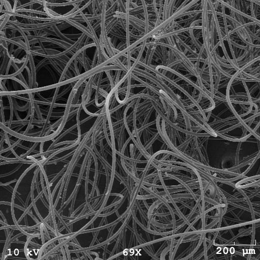
95 25 µm 13 µm 7 µm Figure 6.6 SEM photographs of fibers. 76

96 6.2. Fiber Molecular Orientation The molecular orientation is an important property of fiber since it correlates to fiber crystallinity and mechanical properties. In our process, the fiber is attenuated by air drag force accompanied with cold air cooling. The molecular orientation was built up during the attenuation. To characterize the molecular orientation, two different methods were applied, wide-angle X-ray diffraction and Raman spectroscopy. Raman spectroscopy was chosen as the major technique because of its easy test procedure and data analysis. To validate this application of Raman on fiber molecular orientation, three PP115 fibers with different draw ratio were characterized by both Raman and WXRD. The results are shown in Figure 6.7. In this figure, two fibers were made at 220ºC with draw ratio 330 and 1600; the other fiber was made at 240ºC with draw ratio 360. A Raman spectra of raw PP115 pellet was also included. It was reported the ratio of 841/809 cm -1 band intensity can be used to estimate molecular orientation of isotactic polypropylene fiber [94, 95]. It can be observed that this ratio follows the same trend as the orientation results measured by WXRD. These results indicate that Raman spectroscopy is an effective technique for characterizing the molecular orientation of the fibers produced in this study. 77

97 (a) (b) (c) (d) Raman shift (cm -1 ) Figure 6.7 Typical ZZ polarized Raman spectra of PP115 fibers, compared with WXRD pattern. Fibers were made with different draw ratio at different temperatures (a) 1600 at 220ºC; (b) 330 at 220ºC; (c) 360 at 240ºC; (d) control (raw PP115 pellet). 78

98 PP Raman ratio C 200C 220C 240C Draw ratio Figure 6.8 PP115 fiber molecular orientation estimated by Raman spectra. The ratio of 841/809 cm -1 band intensity is referenced to Raman ratio in this study. The Raman ratio of PP115 fibers was calculated from Raman spectra and plotted against draw ratio as shown in Figure 6.8. Based on the results, several trends can be observed: Firstly, at the same processing temperature, the fiber molecular orientation increases with increasing draw ratio resulted from the higher air drag force. As discussed in previous section, the fiber diameter decreases with increasing air/polymer flow ratio. Therefore, it is believed that the fiber molecular orientation also increases with the flow ratio. Secondly, with the same draw ratio, lower processing temperature generally leads to higher orientation because of reduction of relaxation time. Thirdly, the gradient of Raman ratio over draw ratio decreases with increase in processing temperature which may also be explained by the reduction of relaxation time. When the temperature or draw ratio increases, this linear relation either disappears or the slope decreases. 79

99 6.3. Crystallization Behavior of Resulting Fibers As discussed in the literature review section, the polymer crystallization behavior is crucial during structure formation. In this modified melt spinning process, the spinline dynamics is different from that in melt blowing or traditional melt spinning. The new thermal and mechanical environment along the spinline is expected to affect the fiber crystallization behavior which can finally affect the fiber mechanical properties. In this section, the results on the fiber crystallization behavior are presented with discussion provided on crystallinity, crystal form and crystal size Crystallinity The fiber crystallinity was calculated based on the fusion enthalpy from the DSC tests. Figure 6.9 shows the crystallinity of fibers made from PP115 under various processing conditions. Figure 6.10 shows the results of PP12. No obvious trends were found between the fiber crystallinity and processing conditions. For PP115 fiber, the fiber crystallinity scattered within the region of 50%±3%. It decreased to 42%±2% for PP12 fiber because high viscosity PP12 has longer molecular chains which make them more difficult to crystallize. Since the fibers were produced under various conditions with temperature from 180ºC to 240ºC and air flow rate from 1 cfm to 6 cfm, it is expected that these conditions should somehow affect the fiber crystallinity. The crystallinity measured by DSC may not be accurate because the recrystallization may occur during the heating. Therefore, WXRD test was performed to study the fiber crystallization behavior. 80

100 Air attenuation at 180 C Air attenuation at 200 C Fiber Diameter Crystallinity 80 Fiber Diameter Crystallinity 80 Fiber Diameter (µm) Crystallinity (%) Fiber Diameter (µm) Crystallinity (%) Air/Polymer flow rate ratio Air/Polymer flow rate ratio Air attenuation at Air attenuation at Fiber Diameter Crystallinity Fiber Diameter Crystallinity 80 Fiber Diameter (µm) Crystallinity (%) Fiber Diameter (µm) Crystallinity (%) Air/Polymer flow rate ratio Air/Polymer flow rate ratio Figure 6.9 Crystallinity of resulting fibers made from PP 115 at different temperatures. 81

101 Air attenuation at Fiber Diameter Crystallinity Fiber Diameter (Micron) Crystallinity (%) Air/Polymer Flow Ratio Air attenuation at 200 C Fiber Diameter Crystallinity Fiber Diameter (Micron) Crystallinity (%) Air/Polymer Flow Ratio Figure 6.10 Crystallinity of resulting fibers made from PP 12 at different temperatures. 82

102 The wide-angle X-ray diffraction patterns of PP115 fibers produced under different conditions are presented in Figure In contrast to the DSC results, the WXRD results reveal that fiber crystallinity is related to the processing temperature and the air/polymer flow ratio. The fibers made at three temperatures 180ºC, 220ºC and 240ºC were tested and compared. Although only 2 samples were presented at 180ºC, it can be seen that the crystallinity increases when the air/polymer flow ratio increases from to The same trend was observed for the crystallinity of fiber made at 240ºC. However, at 220ºC, the crystallinity remained nearly constant and showed no dependence on the air/polymer flow ratio. In addition, the fibers made at lower temperatures had higher crystallinity than those made at higher temperatures. It is well known that the crystallization behavior is affected by two competitive factors, the cooling rate and the crystallization rate. In high speed melt spinning, the crystallinity was found to increase with increasing take-up speed because high crystallization rate occurred with high spinning stress and high orientation [87]. In our modified melt spinning process, the high speed cold air temperature is close to the room temperature (25-30ºC) which is well above the glass transition temperature of polypropylene. Although the high speed air flow helps to cool the melt filament fast, it is not sufficient to immediately quench the melt filament. Therefore, as a fast crystallization polymer, the polypropylene filaments still undergo crystallization. Furthermore, the high orientation formed during the attenuation with the assist of cold air cooling also plays an important role in fiber crystallization. An empirical equation can be used to explain the 83

103 effect of crystallization temperature and degree of orientation on the fiber crystallization behavior [24]: K( T, f ) = K( T,0)exp( Af ) = K exp[ 4ln 2( T T ) / D + A( T) f ] (24) max max 0 where K is crystallization rate, A(T) is a positive parameter, f is orientation factor, K max is the maximum crystallization rate, T max is the temperature where maximum crystallization occurs, and D is the half width of K(T) curve. For isotactic polypropylene, K max =0.55, T max =65ºC and D=60, and the equation can be rewritten to: 2 2 K ( T, f ) = 0.55exp[ 4 ln 2( T 65) / A( T ) f ] (25) In the above equation, there is a negative term and a positive term. The cold air cooling in our process makes the temperature close to T max =65ºC. Hence it makes this negative term even smaller. On the other hand, the high orientation will make the positive term even larger. Mathematically, the crystallization rate is increased by the low processing temperature and high molecular orientation. In our process, the orientation increases with increasing air/polymer flow ratio as shown in Figure Consequently, the increase of air/polymer flow ratio will cause increasing crystallization rate which finally leads to the increase of crystallinity. At temperature 180ºC and 240ºC, the significant increases in orientation result in an increase of crystallinity with increasing air/polymer flow ratio. At 220ºC, the resulting fibers exhibit relative higher crystallinity due to the extremely high orientation and modest processing temperature. Only slight increases on crystallinity are observed with the increase of air/polymer flow ratio. This is because that the fiber crystallinity may reach some limited value under those processing conditions. 84

104 180 C 220 C 240 C 13 K 47 µm 10 K 28µm 6 K 26 µm 23 K 38 µm 15 K 20 µm 7 K 20µm 30K 18 µm 45 K 7 µm 50 K 13 µm Figure 6.11 Wide-angle X-ray diffraction patterns of PP115 under various processing conditions. Inside the shaded box, the first number indicates the air/polymer flow ratio; the second one is the resulting fiber diameter. 85

105 Crystal Form and Crystallite Size The WXRD spectra shown in Figure 6.12 exhibits a typical crystal form for fibers made from isotactic PP. Three strong peaks located at 2θ=14.2º, 17.1º and 18.6º indicate the α-monoclinic reflections of 110, 040 and 130 planes. Crystallization of isotactic polypropylene is a complicated process which can form three different crystal forms, α- monoclinic, β-hexagonal and γ-triclinic. The β-hexagonal and γ-triclinic may be formed under fast quench or high pressure or by introducing special nucleating agents. In melt spinning, α-monoclinic is usually obtained under the conditions of mild quench with modest to high spinline stresses. Therefore, the formation of α-monoclinic crystal indicates that the high speed cold air provides mild quench effect on melt filament Intensity (1000 counts) Theta (degree) Figure 6.12 WXRD spectra of typical PP115 fibers made at 220ºC. The crystallite size of 110 plane for PP115 fiber was calculated based on Scherer s equation and the results are listed in Table 6-3. The typical crystallite size is about 120Å 86

106 for the PP115 fiber made at 220ºC. Table 6-3 Crystallite size and 2θ value of 110 plane of PP115 fiber made at 220ºC. PP115 fiber with diameter (µm) 2θ (º) Crystallite size (Å) Fiber Mechanical Properties µm diameter fiber 43µm diameter fiber 20µm diameter fiber 80 Stress (MPa) Strain (%) Figure 6.13 Typical stress-strain curves of single filament. Tensile tests were performed on an Instron machine. The stress-strain curves were recorded for the calculation of tensile strength and tensile modulus. Figure 6.13 shows the typical stress-strain curves observed in a single filament tensile test. With the increase of strain, the fiber undergoes elastic deformation, yielding, necking and strain hardening. 87

107 It was observed that the necking deformation becomes insignificant and finally disappear with the decrease of origin fiber diameter. This can be described as a transition from (a) to (b) to (c) as shown in Figure In this study, curve (a) usually represents fiber with diameter above 50 µm; curve (b) corresponds to the fiber with diameter in the regime of µm; and curve (c) is for the fiber with diameter under 20 µm. The ultimate tensile strength is dependent on the elongation at break because of the strain hardening effect. Therefore, tensile stress at 200% elongation was chosen as the representative strength for compassion in this study. Both strength values were plot against the initial fiber diameter. Figure 6.14 and Figure 6.16 show the single undrawn fiber tensile strength results made from PP115 and PP12 respectively. Figure 6.15 summarizes the tensile modulus of PP115 fibers. For low viscosity PP115, the single filament with diameter of 10 µm can reach tensile strength of 100 MPa and 2.5 GPa. For high viscosity PP12, the tensile strength increases to 140 MPa for single filament with diameter of 25 µm. The tensile strength and modulus showed a dependence on fiber diameter for both PP115 and PP12. This is because fiber mechanical properties strongly depend on molecular orientation and crystallinity which is also a function of molecular orientation in our process as discussed previously. Generally, the increase of orientation will lead to increases in tensile strength and modulus. It was found in our study that the molecular orientation increases as fiber diameter decreases. Consequently, fiber tensile strength and modulus increase with decreasing of fiber diameter. Since the fiber mechanical properties are very sensitive to processing conditions, the tensile strength and modulus scattered around a linear relation with fiber diameter. The outliers 88

108 observed at diameter of 25 µm for PP115 and 55 µm for PP12 represent the fibers made at relatively high temperature with low air drag force. Therefore, the resulting low molecular orientation and crystallinity lead to the low tensile strength and modulus. To obtain high strength fibers, these processing conditions should be optimized in the way to form high molecular orientation: firstly, a modest processing temperature which can provide proper viscosity for enough attenuation and longer relaxation time for overcoming the disorder in molecular orientation; secondly, high air flow to generate high air drag force to enhance molecular orientation. PP115 fibers Tensile strength at break Tensile strength at 200% elongation Tensile strength (MPa) Fiber diameter (µm) Figure 6.14 Tensile strength of PP115 fibers. 89

109 PP115 fibers Initial modulus Modulus 2000 Modulus (GPa) Fiber diameter (µm) Figure 6.15 Tensile modulus of PP115 fibers PP12 fibers Tensile strength Tensile strength at 200% elongation Tensile strength (MPa) Fiber diameter (µm) Figure 6.16 Tensile strength of PP12 fibers. 90

110 6.5. Melting and Crystallization Temperature The melting and crystallization temperature of PP115 fiber were measured by DSC and listed in Table 6-4. The crystallization temperature varies between ºC and ºC with heating and cooling rate at 20ºC/min in DSC. There is no apparent correlation between the processing temperature and fiber diameter. The melting temperature shows some dependence with the processing conditions. At lower processing temperature 180ºC and 200ºC, the melting temperature slightly increases by about 1ºC when the fibers diameter decreases from 70 µm or larger to 30 µm. When processing temperature further increases to 220ºC, uneven broad endotherm peaks with peak maximum at lower temperature side were observed. The uneven broad endotherm peaks were observed to clearly split into two peaks for the fibers produced at 240ºC with diameters less than 15 µm. The first peak located at 165ºC corresponds to the normal melting point of PP115 and the second one appears at about 170ºC. Figure 6.17 shows all types of endotherm peak shapes described. The second endotherm peak located at 169ºC is gradually developed as processing temperature increases and fiber diameter decrease. The appearance of two melting points was also reported in previous studies as discussed in the literature review chapter. Usually, it is caused by the formation of different crystal forms and crystallite size under certain processing conditions, or by the recrystallization during the heating and cooling environment in DSC scanning. 91

111 Table 6-4 Melting and crystallization temperatures of resulting fibers. Processing temperature (ºC) Fiber diameter (µm) T m (ºC) T c (ºC) * * * * * * * *a broad endotherm peak observed 92

112 Figure 6.17 DSC heating thermograms of PP115 fibers with different endotherm peak shapes. WXRD was performed on the fibers with and without double melting peaks to determine if there are new crystalline forms developed. The WXRD spectra patterns are shown in Figure Both WXRD spectra patterns exhibit the typical α-monoclinic crystalline form with strong reflection at 2θ=14.2º, 17.1º and 18.6º. Usually, isotactic polypropylene has β-hexagonal and γ-triclinic crystalline forms with character reflections at 2θ=16.08º for β 300 plane and 2θ=20.1º for γ 130 plane respectively. However, neither of these two reflection peaks was observed in our sample. Therefore, it can be concluded that there is no new crystalline form developed in the resulting fibers. 93

113 1 2 fibers with one melting peak fibers with two melting peaks intensity θ ( ) Figure 6.18 WXRD spectra patterns of fibers with one or two melting peek(s) in DSC. We further investigated whether this double melting peaks phenomenon was caused by the DSC testing thermal environment. Firstly, the sample fiber was heated and then cooled for two cycles at the same rate of 20ºC/min. As shown in Figure 6.17, the double peaks were only observed at the first heating cycle, indicated by the line 4. After another cooling and heating cycle, the double peaks disappeared and only one normal endotherm peak appeared with peak maximum at ºC as indicated by the line 5. Secondly, the sample fibers were tested under different heating rate with the range from 5ºC /min to 40ºC /min. The DSC curves are presented in Figure At small heating rate 5ºC /min, only an uneven endotherm peak was observed. With the increase of heating rate, another peak at higher temperature starts to split out and becomes more obvious at heating rate of 20ºC/min. Then the second peak becomes blunt again as the heating rate increases to 40ºC/min. Overall, the double endotherm peaks can be observed under different heating 94

114 rate in DSC. The recrystallization effect may weaken the appearance of the second endotherm peak under low heating rate. Moreover, the blunt appearance of the second peak under fast heating rate may result from the low resolution at extremely high heating rate since the sample does not have enough time to react. With the two previous steps, it can be confirmed that the formation of double melting peaks is not caused by the DSC testing thermal environment. In other word, the double melting peaks do not result from the recrystallization during the heating process in DSC Figure 6.19 DSC heating thermograms of PP115 fibers made with various heating rate. Based on previous conclusions, it is expected that the double melting peaks may result from the high orientation in those fibers with diameter under 15 µm. A test was designed to prove this hypothesis. Fibers with only one melting peak were manually drawn about 3 times at room temperature to reach a final diameter of 15 µm. Then the 95

115 same DSC scanning procedure was performed on both the drawn and original undrawn fibers. The results are presented in Figure 6.20 for both fibers with 2 heating and cooling cycles. Compared with the original undrawn fiber, the cold drawn fibers showed a broader endotherm peak appears in the first cycle. This broad peak has maximum covering from 165ºC to 170ºC which can be assumed to be the double peak s maximum with further drawing. After another cooling and heating cycle in DSC scanning, the broad melting peak is replaced by a normal single melting peak which is the same as the undrawn fibers Figure 6.20 DSC heating thermograms of cold drawn and original undrawn PP115 fibers. With all these evidences, it is believed that the appearance of double endotherm peaks in DSC is related to the fiber s high molecular orientation. A high orientation may cause some modification on the α-monoclinic crystal structure which is reflected as double 96

116 melting peaks. Moreover, this kind of modification on crystal structure does not lead to a new crystal form Comparisons with Traditional Melt Spinning Fiber Properties Processing temperature (ºC) Table 6-5 Fiber properties of fibers made by traditional melt spinning. Fiber diameter (µm) Raman ratio (ºC) Crystallinity (%) Tensile strength at 200% elongation (MPa) Tensile strength at break (MPa) For comparison, traditional melt spun fibers were produced on our fiber extruder with mechanical drawing. The resulting fibers were characterized to determine their properties, including fiber diameter, crystallinity, tensile strength and molecular orientation. Table 6-5 summarizes these properties of fibers made from PP115 with processing temperature at 180 and 200ºC. These fibers exhibit similar properties as those made by cold air attenuation process. Compared with traditional melt spinning process, the new process could produce continuous filaments with comparable properties Cost Analysis and Possibility of Scale up The use of compressed cold air introduces an additional cost in this new process as compared with traditional melt spinning process. In previous section, the relationship between fiber diameter and air/polymer volume flow ratio was investigated. For example, 97

117 to produce PP115 fibers with diameters of 8 to 25 µm at processing temperature 240ºC, the air/polymer volume flow ratio varied from about to for the air nozzle with tunnel diameter of 5 mm. Respectively, 0.07m 3 air is needed to produce 1 g continuous fibers with diameter of 25 µm and 0.5 m 3 air is needed to produce the same amount of fibers with diameter of 8 µm. The usage of air can be significantly reduced by using a smaller diameter air nozzle or using an extrusion die with multiple orifices. With multiple orifices on a slot die, this new process may be scaled up for industry application to produce continuous filaments or yarns Fibers Made from Nylon 6 Viscsotiy of Nylon C 240 C 250 C 260 C 270 C n* (Pa.s) ang. frequency (rad/s) Figure 6.21 Viscosity of Nylon-6 at different temperatures and angular frequencies. For demonstration, this process was also successfully applied to other polymer materials, including Nylon-6, a widely used polymer in the fiber industry. The melting point of Nylon-6 is about 225ºC according to the DSC test. Figure 6.21 shows the 98

118 viscosity data of Nylon-6 tested at different temperatures. Compared with the viscosities of PP35 at the temperature in the region of 180ºC-240ºC, Nylon-6 has similar viscosities at the temperature in the region of 230ºC-270ºC. Based on previous polypropylene results, fiber diameter is majorly determined by the polymer viscosity. It is believed that the Nylon-6 fibers with diameter of µm can be produced at the temperature in the range of 230ºC-270ºC. Since the processing temperature is limited by the Teflon insulation piece to below 260ºC, the experiments were conducted at three different temperatures: 240ºC, 250ºC and 255ºC. As expected, the fibers produced at low temperatures will have relatively large diameters. Therefore, the major experiments were conducted at 255ºC with various air/polymer flow ratios for comparison. The resulting fiber properties are listed in Table 6-6. Fiber diameters were plotted against the air/polymer flow ratio as shown in Figure The fiber diameter decreases with the increase in flow ratio before it reaches some minimum value at a high air/polymer flow ratio. Both fiber tensile strength and tensile modulus also increase with the increase of flow ratio. The single filament with diameter of 10 µm has a tensile strength of 216 MPa and modulus of 1.2 GPa. Figure 6.23 shows a polarized microscopy image of a single fiber with diameter about 25 µm. It also indicates a uniform distribution of molecular orientation along the fiber surface. 99

119 60 Nylon 6 fiber made at Mean (Micron) Air/Polymer Flow Ratio Figure 6.22 Nylon-6 fiber diameter versus air/polymer flow ratio. 20µ Figure 6.23 Polarized microscopy image of Nylon-6 fiber. 100

120 Temperature (ºC) Table 6-6 Processing conditions and resulting fiber properties of Nylon-6 fibers. Air/ Polymer Ratio Fiber Diameter (µm) Crystallinity (%) Tensile Strength at Break (MPa) Elongation Ratio at Break (%) Tensile Stress at 40% Elongation (MPa) Modulus at 4% strain (MPa)

121 CHAPTER 7 THEORETICAL ANALYSIS AND MODELING OF COLD AIR ATTENUATION IN MELT SPINNING PROCESS 7.1. Introduction and Objectives As discussed in the previous chapter, the experimental results showed that the final fiber diameter depends on the polymer viscosity, processing temperature, polymer and air volume flow rates. Although in Chapter 4, CFD simulations were conducted to analyze the fiber attenuation mechanism under cold air drawing, the mechanism is still not clear because of the limitations of the CFD model. Firstly, it is difficult to incorporate implicit flow and thermal boundary conditions in the CFD model, such as the air drag force and heat transfer on the moving interface between air and polymer which are both related to fiber diameter and air velocity. Secondly, it was observed experimentally that fiber solidification point varies with different processing conditions and material properties which means an iteration of different geometries is needed. Since each specific CFD model has to be based on a fixed geometry. It is not efficient to create these geometries and solve for each model, especially for geometry with high length to width aspect ratio which typically needs a tremendously large number of elements. To address these limitations, we developed a 1-D non-isothermal Newtonian fluid model by solving three basic governing equations numerically using Matlab. The specific objectives of this theoretical modeling were to: Design and validate a computation method to solve the ordinary differential equations derived from basic fluid dynamics governing equations. 102

122 Formulate a 1-D model for the fiber attenuation process under cold air drawing, and obtain reasonable values for input parameters, such as viscosity, air drag coefficient and heat transfer coefficient. Use the formulated model to analyze the fiber attenuation mechanism, mainly the effects of polymer viscosity, processing temperature, polymer and air volume flow rate on resulting fiber diameter. Use the model to predict the final fiber diameter and compare the predicted values with experimental results Literature Review As discussed in Chapters 1, the melt blowing process was developed based on the melt spinning process. In both processes, the polymer melt is extruded out of the extrusion orifice to form a filament, and it is immediately attenuated by external forces. In melt spinning, the external force is the drag force applied by a drawing roller. The air surrounding the fiber applies a retarding force on the fiber. In melt blowing, the external force is provided by a high speed air stream with air frictional force on the fiber surface. Numerical models for melt spinning with air flow as retarding force have been available for some decades. The models for melt blowing were mostly derived from the same governing equations by applying inverse air drag force and different boundary conditions. In this section, the background on modeling melt spinning is introduced first, and a comparison between melt spinning and melt blowing modeling is then presented. The original studies on melt spinning modeling mainly focused on how the fiber is cooled along the spinline during the attenuation process. Andrews [97] set up groups of heat flow equations and solved them approximately with the aid of empirical data. With 103

123 this model, he predicted the temperature profile with the distance from the spinneret for both surface and centerline of the filament. The results were quite accurate, although the predicted radial temperature distribution was only correct to within 20%. A seminal work in this filed was contributed by Kase and Matsuo [57, 58]. They developed fundamental equations on the dynamics of melt spinning. Then steady-state and transient solutions of these fundamental equations were derived and compared with experimental results. The fundamental equations used in their study are: Equation of heat balance: v t t π h t t + = x τ ρ C A * 2 ( ) p (26) Equation of force balance: v F = x β A (27) Equation of material balance: A A v v + = A x τ x (28) In the above equations, x is the distance from the spinneret and τ is the time. Both of them are independent variables. Temperature t, cross-sectional area A and local velocity v are the dependent variables. In their calculations, the tensile viscosity β is assumed only to be a function of temperature t as well as the spinning tension F. One important contribution of their work is the correction of heat transfer coefficient for melt spinning process. They experimentally measured the heat transfer coefficient by hanging a heated wire with diameter of 0.2 mm in an air flow. By recording and converting the cooling of the wire, the Nusselt number was fitted with Reynolds number 104

124 and was compared with other research results as shown in Figure The data fitting turned out a relation of Nu=0.764Re Figure 7.1 Nu vs. Re in cooling by forced convection of cylindrical body; ( ) dataa of Simmons; ( ) data of Mueller; ( ) dataa of Sano and Nishikawa; ( ) Kase and Matsuo s work [57]. However, it was realized by the authors thatt this calculation method can not exactly represent the real heat transfer phenomenon of melt spinning process because the wire was stationary. With further efforts, the authors derived a new Nu-R Re relation Nu= =0.42R Re f for parallel air flow of melt spinning with Reynolds number within the range of Addi itionally, a corrective coefficient (1+K) was multi iplied to the heat transfer coefficient for the contribution of a transverse air velocity correction. The heat transfer coefficient used in their mode del was constructed as: h = 0.21k 1 F π ( A 2G ) π Aρv F (1 1+ K ) (29) 105

125 where K F is the heat conductivity of polymer; G is the polymer flow rate; ρ is the polymer density and µ F is the kinematic viscosity of ambient air. Both steady-state and transient solutions were obtained by solving the listed partial differential equations with the corrected heat transfer coefficient. The results showed a good agreement with the measured experimental data of temperatures and fiber thickness along the spinline. Furthermore, the effects of material properties and processing conditions on final fiber thickness and temperature distributions were also studied. Finally, the steady-state solutions were related to the yarn properties. Specifically, the yarn density, birefringence, crystallinity and molecular orientation were predicted based on the filament temperature and cross-section area. Spruiell et al. [98, 99] developed an inverse model to calculate the heat transfer coefficient and elongational viscosity for high speed melt spinning of Nylon 6. In this inverse model, the fiber diameter, temperature profile and tension at the bottom of the spinline were experimentally measured and used to calculate the rheological force as a function of position along the spinline. The equation used for calculation is: L L 2 2 rheo ( ) = L ρair d π [ ( ) ( )] + ρ π ( / 4) z z (30) F z F C V Ddz W V L V z g D dz where W is mass throughput, V is fiber velocity, F L is take-up force and C d is air drag coefficient. Then a regression analysis was used to fit a smooth function for the fiber diameter and temperature profile. The continuity equation was used to calculate fiber velocity. Finally, the velocity and temperature gradients were obtained by differentiating the smoothed velocity and temperature profiles, and then they were used to calculate the elongational viscosity and heat transfer coefficient. The regression analysis confirmed that the heat transfer coefficient involved in this melt spinning process is not a material 106

126 property. By fitting the calculated heat transfer data versus the ratio of fiber velocity over cross-section area, an empirical equation for heat transfer coefficient was given by: h V A = ( / ) (31) The air drag coefficient is an important coefficient for describing the air drag force applied on the filament during melt spinning and melt blowing. Matsui [100] developed a relationship between the air drag coefficient C f and the Reynolds number Re D based on the turbulent boundary layer theory. C f = β Re n (32) D Re D ρ UD µ a = (33) a where β and n are constant coefficient, ρ a is the air density, µ a is the air viscosity, U the velocity of the filaments, and D the diameter of filament. With β=0.37 and n=0.61, a satisfactory agreement between theoretical analysis and this empirical relation was observed for spinning speed in the range of m/min in melt spinning. Shambaugh and Majumdar [44] designed an instrument to experimentally measure the air drag force under a wide range of conditions. The filament diameter varied from 13 to 305 µm and the air velocity changed from 36 to 300 m/s. The experimental results were found to fit well with an empirical relation: 0.61 C f 0.78 Re D = (34) In this study, they also summarized representative values of β that were determined by various investigators listed in Table 7-1. Based on Kase and Matsuo s effort, more recent studies on modeling of melt spinning expanded the 1-D model to 2-D models. These 2-D models also included the 107

127 combined effects of flow induced crystallization, molecular orientation, non-isothermal viscoelasticity, and air drag. Differential constitutive models were widely used to analyze the melt spinning process, such as upper-convected Maxwell (UCM) model, Phan-Thien/Tanner (PTT) model and Kaye/Bernstein-Kearsley-Zapas (K-BKZ) model. For example, Mitsoulis and Beaulne [101] studied the rheological effects in fiber spinning using numerical simulation with K-BKZ model. The non-isothermal unidirectional model was constructed by the following mass, momentum and energy equations respectively: 2 ρ( π r ) u = ρq (35) d τ zz τ rr du g ρa πu ( ) + C f u( ) = 0 (36) dz ρu dz u ρ Q dt Q Q 4 4 ρc pq + 2 π hc ( T T ) + 2 π σ SBε ( T T ) = 0 (37) dz πu πu with boundary conditions: 1. u = u at z = T = T at z = u = ul at z = L (38) 108

128 Table 7-1Value of β and n from literature [44]. Case β n Maximum V rel (m/min) Fiber diameter (µm) Re D Comments Single filament melt spinning into stagnant air Single and multiple stationary filament inside a tube; tensioned and untensioned Single stationary filament in a tube; untensioned Single stationary filament in a tube; filament not tensioned Single filament melt spinning with no guide at take up roll Single filament melt spinning with guide at take up roll Simultaneous melt spinning of 16 filaments Single stationary filament in wind tunnel or single melt spun filament in wind tunnel Drag exerted by aspirator jet on a filament Drag exerted upon filament by a free annular jet 109

129 where ρ is the density, u is the fiber velocity, Q is polymer volume flow rate, τ represents extra stresses, g is the acceleration of gravity, C f is the air drag force coefficient, C p is the specific heat capacity, h c is the heat transfer coefficient, T is the filament temperature, T is the ambient air temperature, ε is the emissivity, σ SB is the Stefan-Boltzmann constant, and L is the spinline length. Both isothermal and non-isothermal cases were simulated in this study. In the nonisothermal case of PET study, the results showed that PTT and K-BKZ have similar predictive capabilities. It was also concluded that the inertia, gravity, and air drag are important in the simulation. In the case of LDPE study, die swell was found to be very important for predicting the take-up force. Usually, the 1-D model is sufficient to simulate the melt spinning process because the fiber diameter is relatively small compared with the spinline length. In 1-D simulation, the filament temperature is only a function of axial distance from spinneret which means there is no temperature variance in the radial direction. Henson et al. [102] indicated that neglecting the radial temperature variation led to an overestimate of the forced heat convention on the filament surface. This overestimation on heat transfer can cause inaccuracy of the fiber velocity and finally influence the simulation results. Additionally, the radial temperature variation also yielded radially non-uniform tensile stress, which results in non-uniform molecular orientation and crystallinity. Sun et al. [103] confirmed Henson s finding by simulating a 2-D non-isothermal melt spinning case with ongoing crystallization using the commercial software Polyflow. The constitutive equation used in this simulation was the PTT model, which was converted from its isothermal form with a time-temperature superposition algorithm. The simulation 110

130 results showed that the non-uniform thermal history gave rise to a strong radial variation of viscoelastic stress which finally led to a strong effect on the resulting fiber properties, such as crystallinity and molecular orientation. Doufas et al. [61-63, 104] also successfully used a 2-D model to simulate melt spinning including flow-induced crystallization for many polymers, such as PET, PLLA, and rpla. Their results showed good agreement between simulated results and experimental spinline data for the relation between processing conditions and fiber microstructure. Unlike melt spinning, melt blowing is quite difficult to simulate since its lower boundary is a moving boundary and needs to be determined during the simulation. Extensive modeling studies were conducted by Shambaugh and his group [45, 70, 71]. Their first attempt [70] was to develop a 1-D model based on the following continuity, momentum and energy equations: Continuity A v z fz = Q = constant (39) where A z is fiber cross-section area, V fz is fiber velocity and Q is polymer volume flow rate. Momentum d d zz rr z V dv rel fz π d z ( ) j d zc f a f Q f g dz π τ τ π ρ ρ ρ 4 = + 2 dz 4 (40) where z is axial position, τ are extra stresses, C f is air drag coefficient, ρ a is air density, v rel is difference in velocity between the filament and air, ρ f is polymer density, d z is fiber diameter and g is gravitational acceleration. 111

131 Energy ρ dtfz 4hz f Cpf vfz ( Tfz Taz ) dz = d (41) where h z is convective heat transfer coefficient, T fz is filament temperature, T az is air temperature and C pf is heat capacity of the fiber. These governing equations are almost the same as those used in melt spinning simulation. The only difference is the air drag force in the momentum equation, which plays a dominant role on fiber attenuation in melt blowing process. For the boundary conditions, the upper boundary is identical to that of melt spinning, where a constant known value of fiber velocity and temperature are imposed. A freeze point method was used in their study to define the lower boundary condition. The position of fiber freeze was specified at z=5 cm where the attenuation of fiber becomes negligible. It was claimed that the selection of z=5 cm gives good fit to the data and a better converged solution. Compared with the experiments data, this model provided an excellent prediction of fiber diameter profile in the region of high fiber attenuation and slight under prediction on final fiber diameter. The Phan-Thien/Tanner viscoelastic model was also applied in this model to compare with the Newtonian fluid model, but only little difference was found between these two constitutive models. It was pointed out by Shambaugh et al that the high prediction of final fiber diameter in the 1-D model results from the fiber vibration at the distance far away from spinneret. To consider this vibration effect, a 2-D model was developed by Rao and Shambaugh [71]. The previous freeze point method cannot be applied to the lower boundary condition since this 2-D model included fiber vibration. Therefore, a new method called stop point was assumed. At this stop point, the fiber velocity is equal to the air z 112

132 velocity. The predictions based on these two different methods were virtually identical and thus proved the accuracy of the stop point method. By comparing with their previous 1-D model results, the new 2-D model actually made little differences in diameter or temperature predictions. The reason of over prediction of fiber final diameter was attributed to the under predicted fiber vibration amplitudes. However, this model provided a method to estimate the experimental conditions that can cause the fiber breakage. Figure 7.2 Comparison of the predictions of the 3D model with those of the 2D and 1D models [45]. This 2-D model was then expanded to a 3-D model to predict the 3-D motion of a fiber in the melt blowing process. However, the 3-D model still gave similar perditions results as compared with the previous 1-D and 2-D models as shown in Figure 7.2. The turbulence effects was concluded as a possible reason for the under predicted fiber 113

133 vibration amplitude. Both Newtonian and Phan-Thien/Tanner models were used in this study, and the predictions of fiber diameter and temperature showed similar results. In conclusion, the model used in melt spinning can be applied to the simulation of melt blowing process with two modifications: 1. Change the retarding air drag force into forward direction; 2. Use a moving boundary condition for the lower boundary, either stop point method or freeze point method. Based on the literature, 1-D model is satisfactory to simulate the melt blowing process. 2-D and 3-D models do not give better predictions on the fiber diameter and temperature profile although they dramatically increase the computation time. For polypropylene, the Newtonian constitutive model can provide similar predictions as that using the Phan-Thien and Tanner model Model Formulation Model Description In this study, a 1-D non-isothermal Newtonian fluid model was chosen to simulate the melt spinning process under cold air attenuation. Figure 7.3 describes the process and forces acting on the single filament. The air drag force applied on the fiber surface is in the same direction as the gravity force. These two forces are counterbalanced by the rheological force and inertia force. Since cold air was used in this process, forced convection heat transfer occurs on the interface between polymer melt and cold air. 114

134 r die Rheological force Inertia Air Air r Air drag force Attenuation stop point Z Gravity Figure 7.3 Schematic of the melt spinning process by cold air attenuation and the force balance on fibers Governing Equations The continuous filament obeys mass conservation at any position beneath the spinneret orifice. The density of polymer only changes about 10% between the melt and the solid state. Only considering a constant polymer density, the mass conservation can be simplified to volume conservation which means the polymer volume flow rate remain constant anywhere. ρ πr V 2 f f f = ρ Q (42) where ρ f is the polymer density, r is the fiber radium, V f is the fiber velocity and Q is the polymer volume flow rate. The differential form of the momentum equation can be formulated based on the force balance: 115

135 ( ) 2 d V 2 a V f dv f 2 r ( zz rr ) (2 r) C f a f Q r f g 0 dz π τ τ + π ρ ρ + π ρ = (43) 2 dz where τ zz and τ rr are the extra stresses in z and r direction, C f is the air drag coefficient, ρ a is the air density, V a is the air velocity, and g is the gravitational acceleration. The air drag coefficient, C f, is defined by Matsui [100]: C f = β Re n (44) D where Re D, the Reynolds number, is defined by: Re D ( 2 ) ρ V r a a = (45) µ a where β and n are constant coefficient, ρ a is the air density, and µ a is the air viscosity. β=0.78 and n=0.61 are appropriate value for melt blowing based on Shambaugh and Majumdar s study [44]. These parameters are also applicable in our process since air dynamics environment is similar. A simplified steady state energy equation was used in this study: ρ dt f 4hc f C pfv f ( T f Ta ) dz = 2r (46) where C pf is the polymer heat capacity, T f is the fiber temperature, T a is the air temperature and h c is the convective heat transfer coefficient. Because the forced convective heat transfer is dominant, the heat transfer effects resulted from conduction, radiation, viscous heating are neglected. The heat transfer coefficient, h c, can be determined with the following correlation: Nu = γ (47) Re m D where Nu, the Nusselt number is defined as: 116

136 h (2 ) c r Nu = (48) k where k a is the thermal conductivity of air, and the Reynolds number has the same definition as that in Equation (45). γ and m are constants which are equal to and 0.38 respectively according to Matsuo and Kase s study [57]. a Constitutive Equations For a Newtonian fluid, the stress tensor τ zz and τ rr are defined as: τ τ zz rr dv f = 2η (49) dz dv f = η (50) dz where η is the zero shear rate viscosity of the polymer. As a non-isothermal model, the temperature dependence of viscosity is considered using the Arrhenius law by the following equation: For PP η = exp T f (51) For PP η = exp T f (52) where T f is the filament temperature in Kelvin Boundary Conditions Two boundary conditions can be specified for this model. The upper boundary located just beneath the die orifice can be defined as: 117

137 V = V at z = 0 f f 0 T = T at z = 0 f f 0 (53) The lower boundary is located at where the fiber solidifies and the fiber attenuation stops. Unlike the traditional melt spinning whose lower boundary condition is fixed by take-up speed, the low boundary presented in this model is a moving boundary and need to be determined during the calculation. Two conditions based on temperature and velocity are used to define the lower boundary: dv f = 0 at z = L dz T = T at z = L f s (54) where L is an unknown variable defining the position where the fiber solidifies, T s is the fiber solidification temperature which is equal to 135ºC for polypropylene in this study as discussed in the previous part. This lower boundary condition is appropriate to describe the fiber solidification phenomenon since it determines the solidification point based on two variables, the temperature and velocity gradient Method of Solution The governing equations with the substitutions described were solved numerically using MATLAB by finite element method. The detail calculation procedures are: 1. In momentum equation (43), substitute the air drag coefficient with equation (44), the extra stresses with equations (49) and (50). 2. In energy equation (46), substitute the heat transfer coefficient with equation (48). 3. Simplify the substituted momentum and energy equations with mass conservation equation (42), replacing the variable r with function of V f by equation: 118

138 Q r = (55) πv f Then the momentum and energy equations can be simplified in the forms of: 2 2 d Vf dvf dvf = ( f ) ( f f ) ( f f ) f V f T, V f T, V 2 dz dz dz (56) dt ( f )( f a ) f f2 V T T dz = (57) where f(v f ) are functions of variable V f and other constant variables, f(t, V f ) are functions of variables T, V f and other constant variables. 4. Equation (56) is a second order ordinary differential equation. Since it is a one-dimensional model, V f and T f are only the functions of spinline position z. Taking: 1 3 ( ) ( ) y z = y z = V dvf y2 ( z) = y ( z) = dz y z = T ( ) f f (58) The second order ordinary differential equation can be downgrade to first order. The new momentum and energy equations will form a system of three first order differential equations which are solvable in MATLAB with its built-in boundary value problems solver. ( ) ( ) y z = y z 1 2 ( ) ( ) ( ) ( ) 2 ( ) ( ) ( ( ), ( )) ( ) ( ( ), ( )) ( )( ( ) a ) y z = f y z y z + f y z y z y z + f y z y z y z = f y z y z T (59) 5. Two separate iteration schemes were applied during the calculation. The first one is based on the fiber velocity. The iteration will converge on a result that satisfies the initial fiber velocity at upper boundary and velocity gradient at lower 119

139 boundary. In second iteration, the fiber length will be increased step by step. At each step, the fiber temperature at lower boundary will be compared with fiber solidification temperature 135ºC. The iteration will stop if the fiber temperature is lower or equal to 135ºC. Otherwise, the fiber length will be increased for next iteration until the fiber temperature reaches that solidification temperature Validation of Computation Method The MATLAB built-in solver bvp4c was used to solve the system of three first order ordinary differential equations. This computation method was validated using commercial CFD software Polyflow. A simple model was created which can be simulated by both methods. In this model, the fiber freely falls down after extruded out of the die orifice. The only external force acting on the fiber is the gravity force which is the driven force for fiber attenuation. An isothermal incompressible Newtonian fluid was considered to simplify this validation process. The governing equations were formulated as follows for the calculation in MATLAB: Mass conservation ρ Q = ρ π r V (60) 2 f f f Momentum conservation d dv 2 f 2 π r ( τ zz τ rr ) ρ f Q π r ρ f g dz = dz (61) Where the extra stresses is defined as: τ zz dv f = 2η (62) dz τ dv f rr = η (63) dz 120

140 A fixed fiber length was used for each validation case. The upper boundary at the die orifice is V f =0.003 m/s for the initial fiber velocity. The lower boundary at bottom geometry is dv f /dz=0 which means the stop of fiber attenuation. In Polyflow, a rectangular geometry was created and imported as shown in Figure 7.4. An isothermal Newtonian fluid model was chosen and polymer density and viscosity are assumed constant. The width of the geometry was calculated according to the mass conservation equation using the same volume flow rate as that in MATLAB calculation. Four different geometry lengths were generated for the validation, 3 cm, 4 cm, 5 cm and 10 cm. B.C.2: Inlet with Vn=-0.003m/s Flow direction B.C.1: Symmetric axis B.C.3: Free surface B.C.4: Outlet with fn=vs=0 Figure 7.4 Model description of geometry and boundary conditions of freely fall down fiber in Polyflow. The simulation results obtained from Polyflow are shown in Figure 7.5. The fiber geometry was rescaled to get the full view. Under the same external force, gravity, the fiber velocity increases with the increasing of origin geometry length. In other word, the 121

141 longer initial geometry length will lead to higher fiber acceleration and finally results in a finer fiber. When the initial geometry length increases from 3 cm to 4 cm, 5 cm and 10 cm, the final fiber velocity increases from m/s to m/s, m/s and m/s respectively. 122

142 (a) (b) (c) (d) Figure 7.5 Polyflow simulation results for freely fall down fiber model with different model geometry in length, (a) 3 cm, (b) 4 cm, (c) 5 cm and (d) 10 cm. 123

143 Fiber velocity (m/s) cm-Polyflow 3cm-MATLAB 4cm-Polyflow 4cm-MATLAB 5cm-Polyflow 5cm-MATLAB 10cm-Polyflow 10cm-MATLAB Distance from die orifice (m) Figure 7.6 Comparison between the results obtained by Polyflow and MATLAB for different initial geometry length, 3 cm, 4 cm, 5 cm and 10 cm. The simulation results obtained from MATLAB are presented in Figure 7.6 and are compared with the results from Polyflow. In the figure, the circles represent the Polyflow results and the lines represent the MATLAB results. The two results are essentially identical which means the computational methods used in MATLAB are as accurate as that in Polyflow for the test cases. This validation procedure confirms that the calculations based on the model implemented in MATLAB are free from computational errors Isothermal Model Although the objective of this theoretical modeling is to build a non-isothermal model, it is desirable to develop an the isothermal model first for the following two reasons: 124

144 Firstly, the isothermal model provides a better understanding of the effect of processing conditions. With a non-isothermal model, the effects of processing conditions are coupled. For example, the air flow velocity influences both heat transfer coefficient and air drag coefficient. When the air flow velocity increases, the heat transfer coefficient increases and makes the fiber cooled faster which prevents fiber attenuation, whereas the air drag force increases with the increase of air flow velocity thus promoting fiber attenuation. Secondly, it is easier to study the effect of the attenuation stop position in the isothermal model. Usually, dv f /dz=0 is defined as one of the boundary conditions at the attenuation stop point. The second condition on this boundary is to define the position where the attenuation stops. It is expected that different stop positions will generate different fiber velocity profiles and thus affect the whole simulation results. Excluding the effects from energy equation will make it easier to analyze this mechanism. The material properties and processing conditions used in the isothermal model are listed in Table 7-2 except for some specialized individual case. A position with a distance of 5cm from the orifice was chosen initially as the model geometry length. Table 7-2 Material properties and processing conditions for the isothermal model with 5cm model geometry length. Density (Kg/m 3 ) Viscosity (Pa s) Velocity (m/s) Polymer Air

145 Effect of Model Geometry Length As discussed earlier, the simulation results showed that the fiber velocity depends on the model geometry length. Therefore, we first studied the effect of model geometry length on the fiber final diameter. Six different model geometry lengths with range from 1cm to 6cm were simulated and the results were compared in Figure 7.7. The fibers were attenuated to smaller diameters with increase of model geometry length. Within a very short distance from the die orifice, all six cases follow the same trend of fiber diameter versus distance. Then some curves start to split out in sequence with the increase of model geometry length which means that the fiber velocity profile also changes with the variation of model geometry length. This is because the longer model geometry length causes more acceleration in fiber velocity before it reaches the lower boundary. It was observed that the differences between fiber diameters are not significant when the model geometry length goes beyond 3cm which means a converged simulation result. Further investigation indicated that this critical model geometry length varies with material properties and processing conditions. 126

146 Fiber diameter (mm) Fiber diameter (mm) m 0.02m 0.03m 0.04m 0.05m 0.06m Distance from spinneret (meter) Distance from spinneret (meter) Figure 7.7 Isothermal model: fiber diameter profiles with different stop point positions (Inset: magnified view). There is another important observation based on the results from Figure 7.7. Most of the fiber attenuation occurs within about 1 to 2 cm distance from the spinneret orifice in the simulations of different model geometry lengths. For example, in the case of model geometry length of 6 cm, the fiber diameter decreased to about 25 µm after 1cm and reached about 10 µm after 2 cm. After 3cm, the attenuation became insignificant and a flattened region appeared. Within this plateau region, the fiber diameter only changed from about 7 to 6 µm. The plateau regions were also observed in the other cases with different model geometry lengths. The starting position of the plateau region varied with different value of model geometry length. 127

147 Effect of Polymer Viscosity As shown in Figure 7.9, the fiber diameter was found to increase with the increase of polymer viscosity because higher viscosity means higher rheological force. As it counterbalances the air drag force, its high value makes fiber hard to be attenuated. It was found that the fiber diameter is not sensitive to polymer viscosity under simulated isothermal conditions. When polymer viscosity increased from 50 to 500 Pa s, the final fiber diameter only increased from about 7 to 17 µm. This is because a very high air flow velocity was used in this simulation. The high air velocity leads to high air drag force which is dominant over the rheological force. This agrees with the results shown in Figure 7.9. When the air velocity decreased to 20 m/s, a more significant difference of fiber diameter was revealed. Fiber diameter (mm) Fiber diameter (mm) Pa*s 400 Pa*s 300 Pa*s 200 Pa*s 100 Pa*s 50 Pa*s Distance from spinneret (meter) Distance from spinneret (meter) Figure 7.8 Isothermal model: fiber diameter profiles with different polymer viscosity with air flow velocity at 100 m/s (Inset: magnified view). 128

148 Fiber diameter (mm) Pa*s 400 Pa*s 300 Pa*s 200 Pa*s 100 Pa*s 50 Pa*s Distance from spinneret (meter) Figure 7.9 Isothermal model: fiber diameter profiles with different polymer viscosity with air flow velocity at 20 m/s Effect of Initial Fiber Velocity As shown in Figure 7.10, the fiber diameter increases with the increase of initial fiber velocity. The fiber diameter is determined by the equation: V D D V = f 0 0 (64) f where the D 0 is the original die orifice diameter which remains constant in our study. Therefore, the fiber diameter is dependent on the velocity ratio V f0 /V f. Figure 7.11 indicates that the fiber velocity increases with the decrease of initial fiber velocity. As a result, the low initial fiber velocity makes the velocity ratio even smaller and results in a smaller fiber diameter. 129

149 0.05 Fiber diameter (mm) Fiber diameter (mm) Distance from spinneret (meter) 0.01 m/s 0.02 m/s 0.03 m/s 0.04 m/s 0.05 m/s 0.06 m/s Distance from spinneret (meter) Figure 7.10 Isothermal model: fiber diameter profiles with different initial fiber velocity (Inset: magnified view). Fiber velocity (m/s) m/s 0.02 m/s 0.03 m/s 0.04 m/s 0.05 m/s 0.06 m/s Distance from spinneret (meter) Figure 7.11 Isothermal model: fiber velocity profiles with different initial fiber velocity. 130

150 Effect of Air Flow Velocity Fiber diameter (mm) m/s 80 m/s 60 m/s m/s 20 m/s 10m/s Distance from spinneret (meter) Figure 7.12 Isothermal model: fiber diameter profiles with different air flow velocity. The fiber diameter also decreases with the increase of air flow velocity as presented in Figure This is because the higher air flow velocity provides higher air drag force which causes more attenuation on fiber. The final fiber diameter did not show a linear variation with change of air flow velocity. At low velocity range, from 10 to 40 m/s, large variation in final fiber diameter was observed. When the air velocity increases from 60 to 100 m/s, only slight change in final fiber diameter was observed Non-isothermal Model Although the isothermal model provides some understanding of the fiber attenuation mechanism under cold air drag, it is not sufficient to predict the entire process since the heat transfer plays an important role on fiber attenuation. Based on the isothermal model, three modifications were made to develop the non-isothermal model: 131

151 1. Introduce the polymer viscosity dependence of temperature by the Arrhenius law. 2. Introduce the energy equation by considering the convection heat transfer. 3. Determine the fiber solidification point by comparing the fiber temperature with polymer solidification temperature Modification of Calculation Method The iteration method described previously was used to simulate one case of the nonisothermal model of fiber attenuation. The material properties and processing conditions are listed in Table 7-3. Table 7-3 Material properties and processing conditions for non-isothermal case. Density (Kg/m 3 ) Viscosity (Pa s) Thermal conductivity (W/K m) Heat capacity (J/K kg) Initial temperature (K) Initial velocity (m/s) Polymer e 5530/T Air *T is the polymer temperature Figure 7.13 shows the simulation results of fiber diameter and temperature profile along the spinline. It was found that the fiber stops attenuation at a distance of 4 mm from the spinneret orifice and the final fiber diameter is just mm which is far bigger than the experiment result, 8µm. This discrepancy must be caused by calculation mistake or improper calculation method. As discussed in section 7.6.1, the model geometry length has a significant influence on the fiber velocity profile. In this calculation, the model geometry length was initiated at 1mm and then increased gradually with a step size of 1mm. Therefore, the large simulated final fiber diameter is caused by the short model 132

152 geometry length. In the simulation, the fiber velocity gradient initially increases to some maximum value and then decreases to converge to the lower boundary condition (dv f /dz=0). When a short model geometry length is used, the velocity gradient can only reach a very small maximum value and then has to start to decrease to the value 0. On the other hand, the short model geometry length also causes fast cooling on the fiber. The equation below shows the reorganized energy equation: 0.38 dtf π K a 2ρaV a = dz ρ f Cpf Q µ a ( f a ) 0.38 r T T (65) The variable in this equation is r, T f and z. The remaining parameters are constant. It is obvious that the large r value will draw a large temperature gradient which makes the cooling faster. With the short model geometry length, the fiber is quickly cooled down to the solidification temperature, which stops the iterative calculation. Therefore this kind of iteration method is not appropriate to simulate this process. Fiber temperature (K) Fiber temperature Fiber diameter Distance from spinneret (m) Fiber diameter (mm) Figure 7.13 Non-isothermal model: fiber diameter and temperature. 133

153 As discussed in the isothermal model, the fiber attenuation nearly stops after its diameter reaches the plateau region which usually starts at some position very close to the die orifice. Therefore, it is reasonable to use the starting position of this plateau region as the fiber attenuation stop point. To address the problem in the previous model, a manual iteration method was developed. In this method, an initial value of the model geometry length is guessed. Then a non-isothermal model is simulated based on this guessed model geometry length. The simulated fiber temperature profile will then be used to identify the solidification point. If this solidification point exactly falls on the starting position of the fiber diameter plateau region, it proves that the initially guessed model geometry length is correct. If it falls on the attenuation region, it means the initially guessed model length is too small. The value of model geometry length needs to be increased gradually until it matches the value of solidification point. On the other hand, the initial value of model geometry length needs to be decreased if the solidification point falls after the starting position of the fiber diameter flatten region. With this new method, an initial model geometry length was set to 5 cm for the previous case. The selection of 5cm is based on the study of Shambaugh and Uyttendaele [70] whose simulation results showed that it provides a good fit and permits the solution to converge. The simulated results are shown in Figure The solidification temperature of 135ºC corresponding to a solidification position of 1 cm is also the starting position of the fiber diameter flatten region. Based on this method, the final fiber diameter was determined as 7.5 µm which is very close to the experiment result of 6.8 µm. The favorable match with experiment data suggests that the modified method is reasonable to represent our process. 134

154 Fiber temperature Fiber diameter Fiber temperature (K) Fiber diameter (mm) Distance from spinneret (m) Figure 7.14 Non-isothermal model: fiber diameter and temperature with processing temperature at 240ºC and stop point position set at 5 cm Effect of Processing Temperature Figure 7.15 shows the simulation results based on previous case but with a 20ºC decrease in processing temperature. The iteration indicates that 4.5 cm is a proper value for the model geometry length. The decrease in processing temperature causes an increase in polymer viscosity which restrains the fiber attenuation. Hence, the model geometry length shifts from 5 cm to 4.5 cm when the temperature decreases by 20ºC. As expected, the final fiber diameter increases to 11 µm. Therefore, the non-isothermal model also predicts that the fiber diameter decreases with the increase of processing temperature. 135

155 Fiber temperature Fiber diameter 0.5 Fiber temperature (K) Fiber diameter (mm) Distance from spinneret (m) Figure 7.15 Non-isothermal model: fiber diameter and temperature with processing temperature at 220ºC and stop point position set at 4.5 cm Effect of Air Flow Speed The experiments results showed that the fiber diameter decreases with the increase of air flow velocity. Once the air flow velocity exceeds some critical value, the fiber does not attenuate anymore and has reached the final diameter. This is because that the air velocity affects two competing factors: the air drag force and the cooling rate. Both factors increase with the increase of the air velocity. When the air velocity or air/polymer velocity ratio is low to median, the increase of air drag force is dominant over that of cooling rate. Once some critical point is exceeded, the increase of cooling rate becomes significant and comparable with the increase of air drag force. Hence, the competitive effects resulted from these two factors may counterbalance each other and show a negligible influence on fiber attenuation. 136

156 Fiber temperature Fiber diameter Fiber temperature (K) Fiber diameter (mm) Distance from spinneret (m) Figure 7.16 Non-isothermal model: fiber diameter and temperature with air velocity of 10 m/s and stop point position set at 7 cm Fiber temperature Fiber diameter Fiber temperature (K) Fiber diameter (mm) Distance from spinneret (m) Figure 7.17 Non-isothermal model: fiber diameter and temperature with air velocity of 35 m/s and stop point position set at 5 cm. 137

157 The experiment data used here has extremely small polymer flow velocity which means that the air/polymer velocity ratio is extremely high even with air velocity at 20 m/s. Three different levels of air velocity (10 m/s, 22 m/s and 35 m/s) were chosen for the comparative studies, while the other parameters were kept the same as those shown in Table 7-3. The case of 22 m/s was simulated in the previous section and the final diameter was about 7.5µm. For air velocity of 10 m/s, the simulated final fiber diameter was 9.5 µm as shown in Figure When the air speed increases to 35 m/s, the final fiber diameter is 7.0 µm as shown in Figure The simulation results agree with the experimental observations that only a minor change on the final diameter occurs when the air velocity increases from 10 m/s to 22 m/s and to 35 m/s. In addition, the solidification point with temperature of 135ºC was found shifted from 1.4 cm to 1.1 cm and to 0.9 cm when the air velocity increased from 10 m/s to 22 m/s and to 35 m/s. This phenomenon also indicates that the cooling rate increases with the increase of air velocity. 138

158 Effect of Initial Fiber Velocity Fiber temperature Fiber diameter Fiber temperature (K) Fiber diameter (mm) Distance from spinneret (m) Figure 7.18 Non-isothermal model: fiber diameter and temperature with initial fiber velocity at 0.01 m/s and stop point position set at 9 cm. Figure 7.18 shows the simulation results when the initial fiber velocity increased to 0.01 m/s from m/s. The simulation results of the original case with initial fiber velocity m/s is shown in Figure By doubling the initial fiber velocity, the final fiber diameter is found to increase from 7.5 µm to 10.5 µm. As concluded in the isothermal model studies, an increase of initial fiber velocity will cause an increase of final fiber diameter. Meanwhile, the increase of initial fiber velocity also slows down the cooling rate. As indicated in the simulation results, the solidification point shifts from 1.1 cm to 1.9 cm which means a slow cooling rate has occurred. The resulting higher fiber temperature improves the fiber attenuation but limits the decrease of final fiber diameter to 3 µm in this study. 139

159 Comparisons Between Experimental Results and Model Simulation Results The non-isothermal Newtonian model was carried out to predict the fiber final diameter based on the processing temperature, initial fiber velocity and air velocity, as listed in Table 7-4. The data of material properties are listed in Table 7-3, including the density, viscosity, thermal conductivity and heat capacity for both air and polypropylene. Most of the simulated results are close to the experimental results except for the case 1 and 4 which show large deviation from the experiment values. Compared with the remaining cases, these two cases are observed with relatively small air velocity and air/polymer velocity ratio. The small air velocity and air/polymer velocity ratio cause a slow cooling of the filament as observed in the experimental studies. This slow cooling phenomenon was also observed in the simulation. For those two cases, the solidification point with temperature at 135ºC was found located outside of the air nozzle which is about 2 cm in length. Once the air escapes the nozzle channel and exposes to the atmosphere, its velocity will start to decrease dramatically and the air drag force will also vanish after a short distance. In this case, the fiber attenuation stops very quickly and results in a large fiber diameter. However, in the simulation, the fiber will keep being attenuated under the same air velocity outside the nozzle until the temperature reaches the solidification temperature because of a constant air velocity is used in this model. Therefore a smaller diameter was obtained in simulation compared with that in the experimental study. This problem has little effect on the results of cases with high air velocity and high air/polymer velocity ratio. In these cases, the solidification points were found inside the air nozzle by measuring the fiber temperature experimentally and the fiber attenuation was already terminated beyond the fiber solidification point. 140

160 Table 7-4 Comparisons between experimental results and simulation results on final fiber Case Processing temperature (ºC) diameter under various processing conditions. Air velocity (m/s) Initial fiber velocity (m/s) Air/polymer velocity ratio Tested fiber diameter (µm) Predicted fiber diameter (m/s) One approach to address this problem is to take the fiber diameter at the position of actual nozzle length as the final fiber diameter. With this approach, the final fiber diameter is 97 µm for case 1 and 52 µm for case 4 which are closer than the previous predictions. To achieve a better prediction for the cases with small air velocity and air/polymer velocity ratio, the air velocity value used in the simulation needs to be corrected with the actually measured value of air velocity outside the air nozzle. A data 141

161 fitting procedure may be used to correlate the air velocity with its position. With this adjustment, better predictions would be expected. 142

162 CHAPTER 8 CONCLUSIONS AND SUGGESTIONS FOR FUTURE STUDIES 8.1. Conclusions An apparatus has been developed to melt-spin ultra fine continuous filaments with only cold air drawing. Parametric experimental studies were carried out to study the effects of processing conditions on the resulting fiber properties. A theoretical process model was established and used to study the fiber attenuation mechanism under cold air drawing. Polypropylene was used as a model polymer in these studies. From the experimental and theoretical studies, the following conclusions can be drawn: 1. The fibers produced by the new process showed a uniform diameter and a smooth surface appearance. The fiber diameter is highly dependent on the polymer viscosity and the processing conditions, including the processing temperature and the air/polymer flow ratio. The fiber diameter was found to decrease with increasing of air/polymer flow ratio and processing temperature, and with decreasing of polymer viscosity and initial fiber velocity. Fibers with diameter of 7µm were successfully produced from a spinneret with a 0.5 mm diameter orifice. 2. Fiber molecular orientation increases with the increase of air/polymer flow ratio. The maximum molecular orientation was observed at mild processing temperature ( ºC). The fiber mechanical properties were found to correlate with the molecular orientation. The tensile strength and modulus increase with the increase of air/polymer flow ratio. The single filament with diameter of 10 µm (without 143

163 post drawing) exhibits moderately high mechanical properties with a tensile strength of 100 MPa and a tensile modulus of 2.5 GPa. 3. Orientation induced crystallization was found to be dominant in our process. The fiber crystallinity increases with the increase of air/polymer flow ratio accompanied by an increase in molecular orientation. Low crystallinity fibers were found to associate with high processing temperature at relatively low air/polymer flow ratio. Only α-monoclinic crystalline was formed for the produced polypropylene fibers. 4. For further demonstration, this process was also successfully applied to other polymer materials, including Nylon An isothermal Newtonian fluid model was developed to analyze the single factor effect of processing conditions on fiber diameter. A non-isothermal Newtonian fluid model was implemented to predict the fiber final diameter under different processing conditions. The predicted values compare favorably with the experimental data Suggestions for Future Studies The future studies are suggested for the experimental apparatus, experimental studies and theoretical modeling. Apparatus: the processing temperature is limited to below 260ºC because it is the maximum operation temperature of Teflon which is used in the spinneret pack as a thermal insulation. In addition, the fiber is surrounded by the stainless steel spinneret pack which makes it impossible to measure the fiber diameter and temperature online. To 144

164 overcome these limitations, a new design of spinneret pack is proposed to satisfy the following requirements. 1. A high-temperature insulation piece with operation temperature over 400ºC will allow processing some high melting point polymer materials with broad processing temperatures, such as Nylon and PET. 2. A transparent air chamber and air nozzle with access to a high speed camera and an Infrared camera would facilitate online measurement of the fiber diameter and the temperature distribution along the spinline. 3. Several air nozzles with different channel length would provide various cooling times at the same air flow velocity. Experimental studies: with a new experimental setup, a series of experiments can be carried out to study the PET fiber crystallization behavior under cold air cooling and attenuation. As a slowly crystallizing polymer, PET is anticipated to have different crystallization behavior resulted from the different thermal environment provided by cold air cooling. Specifically, the crystallinity of PET fiber can be controlled by changing the air flow speed and the length of nozzle. Theoretically, with high air low, highly orientated amorphous PET fibers may be obtained. Theoretical modeling: 1. Adjust the air velocity in the model with more accurate air velocity profile inside and outside air nozzle for better predictions. 2. The data from online measurements of fiber diameter and temperature profile can be used to validate the modeling results. The air drag coefficient and convection 145

165 heat transfer coefficient may be modified for better predictions based on online measurement data. 146

166 APPENDIX A DRAWING OF SPINNERET PACK A.1. Spinneret Die 147

167 A.2. Air Chamber 148

168 A.3. Air Nozzle 149

169 A.4. Insulation Piece 150

170 151

171 APPENDIX B PICTURE OF FIBER EXTRUDER 152

172 153