Steam Injection Technique for In Situ Remediation of Chlorinated Hydrocarbons from Low Permeable Saturated Zones - Experiment and Numerical Approach

Transcription

1 Universität Stuttgart - Institut für Wasserbau Lehrstuhl für Hydromechanik und Hydrosystemmodellierung Prof. Dr.-Ing. Rainer Helmig Versuchseinrichtung zur Grundwasser- und Altlastensanierung Prof. Dr. rer.nat. Dr.-Ing. András Bárdossy Jürgen Braun Ph. D. Dr.-Ing. Hans-Peter Koschitzky Diplomarbeit Steam Injection Technique for In Situ Remediation of Chlorinated Hydrocarbons from Low Permeable Saturated Zones - Experiment and Numerical Approach presented by cand.-ing. Simon Matthias Kleinknecht Matrikelnummer: Stuttgart, the 18th of January 2011 Examiner: Dr.-Ing. Holger Class, Dr.-Ing. Jennifer Niessner Tutor: Dr.-Ing. Holger Class, Dipl.-Ing. Oliver Trötschler

2 Affidavit Hereby I declare, that i prepared this thesis autonomously withouth illegitimate help and only with the sources duly noted and marked herein. Signature Date

3 Contents List of Figures List of Tables Nomenclature List of Acronyms Abstract V VI VII IX X 1 Introduction Motivation Aim of this Thesis Outline Fundamentals Laws of Dalton, Raoult and Henry Scales and REV Porosity and Saturation Permeability and Darcy s Law Capillary Pressure Heat Transport Properties of Tetrachloroethene Saturation Vapour Pressure Steam Injection Technique General Principles Effect of Thermal Enhancement on Contaminant Tank Experiment Experimental Set-up Sampling and Measurement Devices Temperature Measurement Steam, Soil Vapour and Groundwater Flow Contaminant Concentration Measurement Technical Installations Soil Properties Preliminary Investigations I

4 II Contents Former Experimental Investigation Steam Injection Pressure Energy Balance Calculations Slugtest Experimental Procedure Operating Phases Sampling and Parameter Data Acquisition Strategy Experimental Results Mass Flow Heat Distribution Contaminant Recovery Water Mass Balance Energy Balance Tank Heat Loss Estimation Comparison of 1D Numerical Model and Experiment Follow-Up Investigations Numerical Simulation MUFTE-UG Primary Variables Mathematical Model of a Non-Isothermal System Continuity Equation Energy Equation Model Set-up Two-Dimensional Approach Grid Model Parameters Initial and Boundary Conditions Energy Loss Approach Simulation Results Estimates for Input Parameters Sensitivities of Input Parameters Comparison of Experiment and Simulation Comparison of Heat Distribution Effect of Steam Injection Discontinuity Shortcomings of Model Summary and Conclusion 93 Bibliography 96 Appendix 98 A PCE Concentrations 99 A.1 Groundwater and FLS1 Samples

5 Contents III A.2 Concentration Comparison of SVE and FLS B Slugtest Data 103

6 List of Figures 2.1 Van Genuchten relative permeability - saturation relationship Van Genuchten capillary pressure - saturation relationship Saturation vapour pressure curve of water and PCE Principle of in situ steam injection technique remediation set-up Steam injection methods: steam override & steam sandwich Phase states and equilibrium mechanisms of NAPL-water-air system Determination of azeotropic temperature of PCE-water mixture Side view of tank Top view of tank R&I-Flowchart of steam injection installations R&I-Flowchart of soil vapour extraction installations R&I-Flowchart of experiment Technical installations of the experiment Grain size distribution of site Grain size distribution of M2 and its components PCE concentrations of the saturated zone, taken from Leube (2008) [24] Normalized head over time for injection well I1 and I Flow rates of steam injection and soil vapour extraction Flow rates and temperature of soil vapour extraction and groundwater Flow rates of steam injection, soil vapour extraction, groundwater and condensate tank Flow rates and temperature of groundwater Temperature trends of saturated, low permeable M2 and unsaturated zone Heat distribution plots of remediation experiment (1 18d) Heat distribution plots of remediation experiment (28 63d) Temperature trends of profile J temperature sensors Effect of buoyancy forces on steam propagation (t = 3 & 28 d) Percentage distribution of contaminant recovery Contaminant discharge rate and total sum Contaminant concentration of groundwater and condensate tank Contaminant concentration of soil vapour extraction and groundwater Cumulative contaminant recovery Energy input and output quantities Energy input and output Energy loss percentage of single tank parts IV

7 List of Figures V 3.28 Set-up of 1D model for the tank simulation D model spreadsheet for the simulation of the tank experiment Comparison of temperature trendlines of 1D model and experiment Phase states and mass transfer processes of a 2p2cni model Topview of tank and cross-section Front view of cross-section Numerical steam rate determination approach Grid set-up Refined grid Effects of hydraulic conductivity modification on the heat propagation Effects of porosity modification on the heat propagation Effects of thermal conductivity modification on the heat propagation Effects of model domain energy loss modification on the heat propagation Temperature trend of simulation and experiment Heat distribution: simulation Heat distribution: experiment Heat distribution: simulation Heat distribution: experiment Pressure trend at injection node Effect of steam breakdown on heat distribution Effect of steam breakdown on water saturation

8 List of Tables 2.1 Properties of tetrachloroethene Antoine parameters of water and PCE Effect of temperature increase on properties of PCE Experimental set-up specifications Z-coordinates of temperature sensor profile J Physical parameters of used materials Operating phases Experiment flow rates of operating phases Mass balance of remediation experiment Energy balance of remediation experiment Averaged temperatures of porous medium (t = d & d) Stored energy in porous medium (t = d & d) Heat losses at steady state (t = d) Phase states and primary variables of the 2p2cni model Physical parameters of wetting and non-wetting phase Physical parameters of soils Initial conditions of model domain Dirichlet Boundary conditions at east/west boundary Configuration of M2 parameters VI

9 Nomenclature Symbol Meaning Unit/Dimension J c p Specific heat capacity [ kgk h Enthalpy [J] f Factor [-] k Thermal conductivity coefficient [ W ] mk k f Hydraulic conductivity [ m] s k r Relative permeability [-] l Characteristical length [m] m Mass [kg] ṁ Mass flow rate [ kg s ] x Mole fraction [-] Van Genuchten parameter [-] ṅ Molar flow rate [ mos s ] p Pressure [Pa] q Flow rate [ m3 s q Heat flux [ W ] m 2 r Radius [m] t Time [d] A Area [m 2 ] B General quantity transported with flow D Diffusion coefficient [ m2 s Gr Gravity number [-] H Height [m] K Intrinsic permeability [m 2 ] MW Molecular weight [ g mol Nu Nusselt number [-] P r Prandtl number [-] Q Energy flow rate [W ] Q Energy [kj] Ra Rayleigh number [-] S Saturation [-] T Temperature [K] V Volume [m 3 ] X Mass fraction [-] Greek Symbols: α Heat transfer coefficient [W/m 2 K] Van Genuchten parameter [ 1 P a VII

10 Symbol Meaning Unit/Dimension δ Wall thickness [m] ɛ Emission ratio [-] λ Thermal conductivity [ W ] mk µ Viscosity [ kg sm ] φ Porosity [-] ϕ Angle [ ] ρ Density [ kg ] m 3 σ Stefan-Boltzmann constant [-] ϑ Reference temperature [K] Γ Ω Boundary of control volume Control volume Indices: w c l g pm pw r s α κ Water Capillary Loss Gas Porous medium Pore water Residual Radiation Soil Phase Component VIII

11 List of Acronyms 2p2cni 3p3cni AGL BC C-UZ D/C E GC-PID GW HDPE I IWS NAPL PCE SERDP SI SVE TCE VEGAS VZ 2 phase 2 component non-isothermal model 3 phase 3 component non-isothermal model Above ground level Boundary condition Condensate extraction from unsaturated zone Discharge Extraction Well Gas chromatograph-photoionization detector Groundwater High density polyethylene Injection Well Institut für Wasserbau Non aqueos phase liquid Perchloroethylene (tetrachloroethene) Strategic Environmental Research and Development Program Steam injection Soil vapour extraction Trichloroethylene Versuchseinrichtung für Grundwasser- und Altlasten sanierung Vadose zone IX

12 Abstract Steam injection is a commonly applied technique to enhance soil vapour extraction for the remediation of contaminants in the subsoil. However, steam propagation is highly dependent on the permeability of the soils. This thesis describes investigations regarding the heat distribution in a low permeable, saturated zone and the contaminant removal efficiency. To this end, a large-scale tank experiment with two distinct steam injection methods was conducted: 1. steam injection in the saturated zone below the low permeable zone (override) and 2. an additional injection into the unsaturated zone (sandwich). The observed heat distribution was compared to 1D and 2D numerical simulations to evaluate reproducibility and applicability for dimensioning of field applications. The experiment demonstrated the successful heating of the low permeable, saturated layer (thickness of 1.5 m) to about 90 C at the top of the layer after 16 days using the steam override method. A constant steamed zone below the low permeable zone was observed. The additional steam injection in the unsaturated zone showed only a limited effect on the heat distribution in the low permeable layer and achieved no significant increase in contaminant removal. A total mass of 3 kg of contaminant (46% of initial amount) was removed from the subsoil. 88% was removed by the soil vapour extraction, 11% by the groundwater outflow and 1% by the extracted condensate from the unsaturated zone. Contaminant concentrations decreased by 99% in the soil vapour extraction and by 85% in the groundwater. A persisting contamination of the saturated zone was evident. The 1D model was not able to simulate the predominated conductive heating correctly and further model modifications regarding the relevant processes for heat distribution were necessary. The 2D numerical model reproduced satisfactorily the heat distribution in the low permeable, saturated layer for an adapted set of parameters. However, shortcomings resulted from the negligence of the third dimension and the estimation of the heat losses via the boundaries. Hence, the model can not be applied for different configurations of parameters and further investigations and calibration efforts are required. X

13 1 Introduction 1.1 Motivation Water is and will always be the most important resource to maintain a living planet. Due to the rising population over the last decades and, therewith, a significant rise in water consumption, it is every day more important to conserve the quantity of the underground water supply, but even more its quality. The main part of our drinking water is gained by the extraction of groundwater out of aquifers in the subsurface. However, aquifers are often endangered by contaminations caused by, e.g. industrial waste or accidents which release hazardous substances into the environment. Once a contamination in the subsurface is detected the legal situation demands actions to re-establish its previous state and prevent further contamination. The most common contaminants are the so-called non aqueous phase liquids (NAPL). NAPLs denote mostly chlorinated solvents, aromatics, oils and polyaromatics which are immiscible and low soluble in water. In relation to the density of water one distinguishes between lighter (LNAPL) and denser (DNAPL) NAPLs. These show a different behaviour in the subsoil. LNAPLs tend to accumulate on the groundwater surface in the aquifer, leaving a trace of residual saturation behind, while DNAPLs may penetrate through unsaturated and saturated zones until a confining layer is reached, accumulate there and diffuse slowly into it. This behaviour of DNAPLs causes difficulties during an in situ remediation of low permeable layers, hence, different remediation techniques have been developed during the last decades. Comprising for example, pump and treat, soil vapor extraction (SVE) or thermally enhanced SVE. One of the most promising technique is steam injection into the saturated as well as the unsaturated zones of the subsoil combined with soil vapour extraction to remove the prevailing contaminants. Steam has proven as a very efficient way of injecting energy into subsoil. The purpose is to heat the subsoil and, thereby, enhance the remediation. Hence, the heat distribution in the subsoil is of main importance for the remediation processes. My thesis, therefore, addressed in particular the issues of heat distribution in the subsoil. 1

14 2 Introduction 1.2 Aim of this Thesis This thesis has three major aims. The first part is the realization of an in situ remediation of a tetrachloroethene contamination by means of enhanced soil vapour extraction with the steam injection technique. A former physical model, cf. Hiester & Baker (2009) [19], was selected to conduct the large scale experiment in the VEGAS facility. A specific focus will be on the heating process of a low permeable layer in the saturated zone where convective heat transfer is reduced due to the lower permeability. Further, the necessary steam injection rate (energy input) as well as the time duration of the heating process are of interest. Besides the recovery of the contaminant, the main criterion of the experiment is the maximum temperature at the top of the low permeable layer. The target temperature of 90 C was chosen as the boiling point of the water-tetrachloroethene mixture is at 88 C. The second main focus will be on the build-up of a two-dimensional, two-phase, two-component, non-isothermal model to simulate the heat distribution observed in the experiment. The third aim is the comparison of the heat distribution of the experiment with the results of the two dimensional numerical simulation and a one dimensional numerical model which was set up by Guidry (2010) [15]). The distinct aims can be listed as follows: 3D experiment to monitor the heating efficiency of the low permeable zone Applied steam injection methods: override and sandwich Variation of fluxes to enhance the recovery Comparison of the steam injection methods for prediction of: Heat propagation Remediation time Remediation efficiency control Reduction of emissions Mass removal Build-up of 2D numerical model Comparison of heat distribution of experiment with 1D numerical model 2D numerical model

15 1.3 Outline Outline This thesis is divided into three main parts, namely fundamental comments (Ch. 2), the experiment (Ch. 3) and the numerical simulation (Ch. 4). Chapter 2 provides an overview of the definitions of physical and thermodynamical quantities which are the theoretical background for processes occurring during the experiment. These theoretical considerations will form the basis for the numerical model. In addition, physical and chemical key parameters of tetrachloroethene as well as principal methods of steam injection as a remediation technique are given and explained in detail. Chapter 3 addresses the tank remediation experiment including description of the set-up parameters, the procedure and the discussion of the results. The numerical simulation is depicted in Chapter 4. The set-up of the numerical model considering key parameters, primary variables and balance equation is explained and the results gained from the simulations are discussed. 5) com- Finally, a summary and the conclusions gained from this thesis (Ch. plete the work.

16 2 Fundamentals In order to describe and analyze the complex physical processes and align soil remediation by heat treatment, it is necessary to introduce certain concepts such as a description of the system on a specific scale. The scale is based on a predefined degree of abstraction and characterizes the accuracy of the reproduction of processes. The experiment and the numerical simulation are based on thermodynamical, physical and mathematical concepts and definitions which are partly introduced in this chapter. For further information on thermodynamic definitions, cf. Baehr and Kabelac (2010) [5]. Bear and Cheng (2010) [7] give detailed insight on fundamentals necessary for groundwater flow and contaminant transport modelling. 2.1 Laws of Dalton, Raoult and Henry Dalton s Law Dalton discovered in 1805 that the pressure of a gas mixture is equal to the sum of the partial pressures when ideal gases are considered. In the majority of cases the gas phase of a multiphase system consists of various gas components. Daltons s law is then written as p g = p κ g. (2.1) κ Laws of Raoult and Henry In multiphase systems a state of equilibrium is reached after a certain time for each component in each phase. This follows the definition of the thermodynamic equilibrium. At any point in time, the concentration of a substance in the gas phase can be described by means of its partial pressure p κ i, following the ideal gas law. The total gas phase pressure can be determined following Raoult (Eq. 2.2) or Henry (Eq. 2.3), respectively. p g = p κ satx κ (2.2) κ p g = κ H κ αx κ (2.3) Where p κ sat denotes the saturation vapour pressure of the component, H κ α the Henry coefficient of the component κ in phase α and x κ its mole fraction. Generally, Raoult s law can be applied to mixtures of chemically similar components. However, real mixtures show a deviation from the ideal behaviour and, therefore, Raoult s law is only 4

17 2.2 Scales and REV 5 valid for x κ 1. Hence, Henry s law has to be introduced and has to be applied for x κ Scales and REV A porous medium is defined as a portion of space that is occupied by a number of phases of which at least one is a solid. The space within the porous medium which is not occupied by the solid matrix is called void space or pores and filled with one or more fluids or gases (Bear and Cheng (2010) [7]). As already mentioned above, it is not possible to consider every process in every single pore of the porous medium due to differences in geometry even over small distances and the overwhelming complexity. Therefore, processes in a porous medium have to be considered on different scales, for example the molecular scale, the microscale or the local scale, depending on which mechanisms are of interest. On the local scale, a continuum approach is applied in which micro-scale parameters of the porous medium are integrated over a REV (Representative Elementary Volume). This yields an averaged flow description. The size of a REV has to be larger than the size of the heterogeneity but also small enough for spatial variations of the considered properties. This leads to averaged macroscopic values such as the porosity φ and saturation S α, cf., for example, Helmig (1997) [16]. 2.3 Porosity and Saturation Porosity φ denotes the pore space of the porous media available for the fluids and gases. It is defined as the ratio of the pore volume V P ore to the entire volume of the porous media V. φ = V P ore (2.4) V The saturation is defined as the ratio of the fluid volume V F luid to the volume of the pore medium. The term saturation has to be introduced because a determination of the exact spatial distribution of a fluid in the porous medium is not feasible. If more than one phase α is present in the REV, the saturation of phase α is defined in the following way: S α = V α. (2.5) V P ore Considering more than one phase in the REV results in the constraint: S α = 1 (2.6) α Various material laws, e.g. relative permeability-saturation relation, do not refer to the saturation S α, but to the effective saturation S e,α denoted as the portion of a fluid displaceable by hydrodynamical processes. S e,α = S α S αr 1 S αr (2.7)

18 6 Fundamentals Residual saturation can be explained as follows. If a fully water saturated porous media is drained by a non-wetting fluid, e.g. a NAPL, a displacement of the entire amount of water can not be achieved as water is trapped in tiny pores by capillary pressure. The remaining amount of the not displaceable water denotes residual saturation. Furthermore, if the injected non-wetting fluid then is displaced by water also residual saturation remains in the porous media. The processes responsible for this behaviour are discussed in detail in Helmig (1997) [16]. This explains the definition of the effective saturation S e,α. 2.4 Permeability and Darcy s Law The permeability also denoted as hydraulic conductivity, characterizes flow behaviour of fluids in a porous medium or hydraulics, respectively. It was introduced by Darcy in 1856 and is defined as the ease with which fluids can move through pore spaces. The general Darcy equation is defined as v = k f h, (2.8) where v is the velocity in [ m], k s f the proportionality factor in [ m ] and h the hydraulic s gradient [ m]. m Equation (2.9) demonstrates, that the hydraulic conductivity is not only a soil parameter but also depends on the fluid itself. k f = K ρ g µ (2.9) Where the intrinsic permeability K [m 2 ] is a property of the soil and the density ρ and the dynamic viscosity µ of the fluid. Darcy s law (Eq. 2.8) is applied to calculate the flow of a fluid in a porous medium. However, considering multiphase flow one has to modify Equation (2.8) taking into account the resistance one fluid has on the mobility of the other(s). This implies the definition of the relative permeability which can be introduced as a reduction factor of the permeability in Darcy s law. k r,α varies between 0 and 1 at which a single phase condition is determined by k rα = 1. The extended form of Darcy s law is then written as v α = k r,α µ α K ( p α ρg). (2.10) It is common to replace kr,α µ α by λ α which is denoted as the mobility of the fluid. Considering two-phase flow, various approaches to quantify the relative permeabilitysaturation relation can be found in the literature. The approach developed by Van Genuchten is among the most famous and also implemented into the numerical

19 2.5 Capillary Pressure 7 model introduced in Chapter 4. Relative permeability - saturation relationship is determined following two equations, one for the wetting (Eq. 2.11) and one for the non-wetting (Eq. 2.12) phase, respectively. k r,w = [ S e 1 ( ) 1 S 1/m m ] 2 (2.11) k r,n = (1 S e ) 1 3 e [ ] 1 S 1/m 2m e (2.12) 1 1 0,9 0,9 0,8 0,8 Relative Permeability [-] 0,7 0,6 0,5 0,4 0,3 0,7 0,6 0,5 0,4 0,3 0,2 0,1 krw krn 0,2 0, ,1 0,2 0,3 0,4 0,5 0,6 0,7 0,8 0,9 1 Saturation [-] Figure 2.1: Relative permeability - saturation relationship for VG-parameters n = 6, α = 0.6 and S w,r = 0.19 (porous medium (site 3 ) of saturated and unsaturated zone; cf. Troetschler et al. (2004) [32]) 2.5 Capillary Pressure The presence of immiscible fluids in a state of equilibrium within, e.g. a capillary tube, results in a pressure difference between the wetting and the non-wetting phase. This behaviour can be explained by the effect of a fluid to minimize its surface in order to be in a state of minimized free energy. The resulting pressure difference between the fluid that occupies the concave side of the interface and the one that occupies the convex side is defined as capillary pressure. p c = 2γ wncosθ R (2.13) where γ wn denotes the interfacial tension between the fluids, cosθ the contact angle and R the tube s radius. The wetting-phase tends to be as close to the solid as possible.

20 8 Fundamentals In contrary the non-wetting phase minimizes its contact with the soil surface. p c = p non wetting p wetting (2.14) In porous media, one relies on constitutive relationships in order to determine capillary pressure on a local scale. The saturation of the wetting phase is of importance in this aspect as a result of the affinity of the wetting phase to the solid matrix. As a result of this, for small saturations, the wetting phase accumulates first in the narrow pores before occupying the larger ones and vice versa considering the non-wetting phase. Consolidating this observation with Equation (2.13), one can state that for low wetting phase saturation the capillary pressure is accordingly high because of the smaller pore radius. An approach for the determination of the capillary pressure as a function of the wetting phase saturation on a local scale was developed by, e.g. Van Genuchten following, p c = 1 ( ) S 1 1 n m e 1. (2.15) α S e denotes the effective saturation (2.7), n expresses the uniformity of the soil (a high value of n characterizes an uniform soil) and α is considered a scaling parameter of the capillary pressure s magnitude. The correlation between n and m follows m = 1 1 n (Class (2001) [10]) Capillary Pressure p c [kpa] Site ,1 0,2 0,3 0,4 0,5 0,6 0,7 0,8 0,9 1 Saturation S w [-] Figure 2.2: Capillary pressure - saturation relationship for VG-parameters n = 6, α = 0.6 and S w,r = 0.19 (porous medium (site 3 ) of saturated and unsaturated zone; cf. Troetschler et al. (2004) [32])

21 2.6 Heat Transport Heat Transport The main interest of this thesis lies on heat transport in the aquifer and the low permeable zones. The relevant processes, concerning this matter, are introduced in the following. Heat describes the energy transferred over the system boundary. It is forced only by a temperature gradient between the system and the environment, cf. Baehr and Stephan (2010) [6]. Considering heat transport, one distinguishes between heat conduction, convection and radiation. In an aquifer heat is distributed mainly by conduction, through fluids and the soil matrix, and convection, i.e. flow of fluids. Whereas in solid matter heat can only be transported by conduction. In general, radiation can be neglected in porous media. Radiation and convection are considered in order to estimate heat losses via the tank walls. Concerning heat transport, absolute temperature T in most cases plays a minor role, and is replaced by the temperature difference ϑ = T T 0 (2.16) where t 0 denotes the reference temperature and can be chosen independently. Setting the reference temperature to T = K, corresponding to 0 C, is convenient to use the temperatures in C. Heat Conduction Heat is transfered by adjoining molecules as a result of a temperature gradient in the matter. Hence, heat conduction in fluids and solids is of higher importance than in gases due to the smaller intermolecular distance. This results in a heat flux defined by Fourier written as q = λ ϑ. (2.17) The factor λ is a material property influenced by temperature ϑ and pressure p. To determine the thermal conductivity of a porous medium, different calculation approaches exist. The approach by Somerton (1974) [31] based on a root function was chosen also to be implemented in the numerical simulation following λ pm = λ S W =0 pm + S W (λ S W =1 pm λ S W =0 pm ), (2.18) where λ S W =1 pm and λ S W =0 pm denote thermal conductivity of the porous medium at fully saturated and unsaturated condition, respectively. Heat Convection Heat convection is based on transport induced by macroscopical movement of a fluid, cf. Baehr and Stephan, 2010 [6]. It has to be differentiated between free and forced movement. Free fluid movement is a result of buoyancy because of the difference in

22 10 Fundamentals density generated by the different temperatures within the fluid. Whereas forced convection is caused by external forces such as pumps, turbines or phase transformations, e.g. boiling. The considered heat flux q [ W m 2 ] at a wall then can be determined by q = α(ϑ W all ϑ F luid ). (2.19) Equation (2.19) introduced the heat transfer coefficient α as a function of the fluid properties, the fluid flow and the geometry. The heat transfer coefficient can be calculated by the correlation of Nusselt. Nu = αl λ i (2.20) With the dimensionless Nusselt number Nu, the thermal conductivity of the fluid λ F luid [ W ] and the characteristic length l [m]. The determination of the Nusselt number mk Nu = f(p r, Gr) is based on empirical approaches and can be calculated by means of the Grashof number and the Prandtl number (2.22). The product of Grashof number and Prandtl number is also known as Rayleigh number (Eq. 2.21), Ra = Gr P r = β F luidg(ϑ W all ϑ F luid )l 3 ν 2 P r, (2.21) where β F luid for ideal gases follows β F luid = 1 T F luid. Prandtl number for the corresponding fluid parameters is defined as P r = ηc p λ. (2.22) Heat Radiation The main difference between heat radiation and conduction/convection is the fact, that no matter is needed to transport the heat. Further it is determined by the emissivity of the participating bodies, radiating electromagnetically. The emission of a radiating solid body is limited by its thermodynamic temperature. The maximal heat flux, radiating from the surface of a body, has been defined by Stefan & Boltzmann, cf. Baehr and Stephan (2010) [6] in the following way q = σt 4, (2.23) where T [K] denotes the thermodynamic temperature of the body. The universal Stefan-Boltzmann constant is defined σ = ( ± ) 10 8 W [ ]. A m 2 K 4 body which reaches the maximum of Equation (2.23) is called full radiator. Not only radiating, but also absorbing perfectly, it can not be exceeded by another body with the same temperature. This fact introduces the emission ratio ɛ 1 as a function of material properties, which reduces the radiation for a real body, cf. Eq. (2.24). q = ɛ(t )σ (T 4 1 T 4 2 ) (2.24)

23 2.7 Properties of Tetrachloroethene Properties of Tetrachloroethene Tetrachloroethene (PCE) denotes a chlorinated hydrocarbon solvent. Commercially used as dry cleaning or degreasing agent, as a solvent for gases and fats and as a heat-transfer medium, for example. At normal conditions, PCE is liquid and highly volatile. The importance of PCE as an industrial product reflected in the frequency at contaminated industrial sites and, therefore, ranks among the main contaminants of groundwater resource. It is furthermore classified as a DNAPL. Considering these circumstances, PCE was chosen as the representative contaminant in the experiments. Therefore, the main physical, chemical and thermodynamic properties of PCE, of importance for the remediation processes are presented. Property values are taken from the Handbook of Chemistry and Physics (2010) [25] and the Risk Science Program Report (1994) [3]. Table 2.1: Properties of tetrachloroethene Description Symbol Unit Value Chemical formula C 2 Cl 4 CAS-NR Molecular weight MW [ g mol g Density ρ [ ] cm Solubility in water S [ mg L 287 Vapour pressure at 25 C V P [P a] 2600 Henry s law constant H [ P a m3 mol ] 1460 Boiling point at bar T B K Enthalpy of evaporation at 100 C h v [ kj kg Diffusion coefficient in pure aire D Air [ m2 d 0.66 Diffusion coefficient in pure water D W ater [ m Distribution coefficient in: d ] Groundwater-zone soil K d q [ ] K oc 1 f oc s 2 Vadose-zone soil K d v [ ] K oc 1 f oc q 3 1 Soil organic carbon partition coefficient K OC = 160, cf. Karickhoff (1981) [21] 2 Fraction organic carbon in the groundwater-zone soil 3 Fraction organic carbon in the vadose-zone soil

24 12 Fundamentals 2.8 Saturation Vapour Pressure Saturation vapour pressure is strongly related to the temperature and of importance considering phase transition (e.g. vaporization and condensation) and phase change (e.g. displacement or change in pressure/temperature). Taking into account these processes, one has to consider that a chemical compound, appearing in the gas and in the liquid phase is dependent on its mole/mass fractions and interaction between the phases. To be able to describe the occurring physical processes, laws of Dalton and Raoult are consulted, cf. Section 2.1. The saturation vapour pressure curve divides the liquid phase and gaseous phase (steam) area. In Figure 2.3 the saturation vapour pressure curves of water and tetrachloroethene are given, using the Antoine equation, B p sat = 10 A T +C, (2.25) where A, B and C denote empirical parameters. Table 2.2 contains the parameters for water (Dortmund DataBank [1]) and PCE (Reid et. al (1987) [29]). Table 2.2: Antoine parameters of water and PCE Substance A B C Water PCE Vapour Pressure [bar] Water PCE Temperature [ C] Figure 2.3: Saturation vapour pressure curve of water and PCE

25 2.9 Steam Injection Technique Steam Injection Technique General Principles The injection of steam was developed originally by the petroleum industry to increase the recovery of oils from the ground repositories. Nowadays, steam injection is used as a remediation technique for chlorinated solvents in subsoils, enhancing soil vapour extraction. Taking advantage of the heat capacity of steam to achieve a higher heat input than hot air, for example, providing dissolution, vaporization and mobilization of contaminants and thereby a more efficient recovery. One essential aspect considering steam injection is the distinct behaviour of the heat propagation in unsaturated and saturated zones due to the influence of buoyancy. In the saturated zone the density of steam and the liquid water of the aquifer differs significantly, whereas in the unsaturated zone the difference of density of steam and ambient air is of minor difference. The vertical-oriented buoyant forces interact with the viscous forces induced by the steam injection (pressure), responsible for the radial propagation of the steam. Considering this, the shape of the steam propagation is dominated by the ratio of the viscous forces to the buoyancy forces. This ratio is defined as the dimensionless gravity number (Gr) by Van Lookeren (1983) and has been modified for steam injection into an unconfined aquifer by Ochs (2007) [28]. Generally, the standard remediation set-up consists of soil vapour and/or groundwater extraction wells located at the contaminated zone surrounded by steam injection wells or vice versa. Figure 2.4 gives an example of the principle of a remediation set-up using the steam injection technique, demonstrating the difference the saturated and unsaturated zone have on the propagation. For further information on engineering considerations of remediation set-up, cf. Trötschler et al. (2004) [32].

26 14 Fundamentals Figure 2.4: Principle of in situ steam injection technique remediation set-up, taken from Class (2001) [10] Former investigations on heat propagation with steam injection, for example Färber (1997) [14] already characterized the processes, occurring in the subsoil where steam is injected. Saturated steam enters the subsoil and condenses as the surrounding sand particles are still cold. This can be explained by the definition of saturated steam: a finite change in temperature is sufficient to trigger condensation. While condensing, the steam transfers its enthalpy of vaporization to the subsoil, heating the sand particles up to boiling point of water. The relatively high heat transfer during condensation provides a stabilization of the condensation front as steam can only pass regions already at boiling point of water, impeding disequilibrium between the gaseous, liquid and solid phase. The steam is distributed mainly by convection, passing the porous media until it reaches the area where the condensation takes place and the heat is passed to the colder regions. This area is a more or less definable transition zone called steam front. The steam front is characterized by high contaminant concentrations in the vapour phase behind the front and the aqueous phase ahead of the front pushing towards the extraction wells. Inside of fluids and between sand particles one can observe heat conduction, but only at the steam front, as a temperature gradient is necessary following the definition of Fourier. In low permeable zones convection is reduced and other processes, such as thermal diffusion and heat conduction are dominating. However, steam injection is limited by the permeability of the subsoil and best applicable to zones of moderate to high permeability. Guidry (2010) [15] investigated heat distribution in the low permeable zone by steam injection from below in a two-dimensional experiment, demonstrating applicability but also constrictions.

27 2.9 Steam Injection Technique 15 The experiment includes the investigation of two different steam injection techniques, denoted as steam override and steam sandwich. Both techniques take aim at the heating of the low permeable saturated zone in order to exceed a temperature of about 90 C within the zone. The relevant processes for heat distribution are heat conduction or diffusive convection, respectively. During steam override, steam is injected into the saturated zone below the low permeable zone. The steam sandwich includes additionally the steam injection into the unsaturated zone above the low permeable zone. Both methods are illustrated in Figure 2.5. Figure 2.5: Steam injection methods: steam override & steam sandwich

28 16 Fundamentals Effect of Thermal Enhancement on Contaminant The injection of heat has an enormous effect on the key physical and chemical properties of the organic contaminants, benefiting a more or less significant change in fate and transport (EPA (2004) [4]). Figure 2.6 describes the phase transition mechanisms of a NAPL to reach the state of equilibrium, considering three phases and three components. Figure 2.6: Phase states and equilibrium mechanisms of NAPL-water-air system (Class (2001) [11] The properties of PCE given in Table 2.1 are generally based on normal conditions, means 25 C. Table 2.3 derived from Davis (1997) [13] demonstrates changes in properties of PCE at increasing temperature. Table 2.3: Effect of temperature increase on properties of PCE Property Liquid density Vapour pressure Liquid viscosity Solubility Henry s coefficient Partion coefficient Degradation Effect decreases moderately (less than 100 percent) increases significantly (10 to 20 fold) decreases for T < T boiling increases as temperature increases increases (more likely to volatilize from water) decreases (less likely to partition to organic matter in soil) increases

29 2.9 Steam Injection Technique 17 The mentioned changes in properties present positive effects on the remediation (Davis (1997) [13]). For example, liquid viscosity decreases about 1% per 1 C of increased temperature up to the boiling point, enhancing the mobility of PCE. Furthermore, as temperature increases, also vapour pressure increases exponentially and PCE tends to partition to the gas phase. The mass of chlorinated solvents occupies a larger volume in the gas phase than in the liquid phase, resulting in expansion and advective flow. Solubility in water increases by a factor of two or more and the partitioning from the aqueous phase to the soil is generally decreased at higher temperature. One of the main benefits which thermal effects have on the remediation progress is the reduced boiling temperature of the mixture of chlorinated solvent and water, featuring heterogeneous azeotropic properties. This is marked by the boiling of the mixture at a constant temperature (azeotropic temperature) without a corresponding change in composition. The azeotropic temperature can be determined by the method of Badger-McCabe. The intersection point between the vapour pressure curve of PCE and the curve obtained by subtracting the vapour pressure curve of water from the atmospheric pressure curve, determines the azeotropic temperature (cf. Figure 2.7). The azeotropic temperature of a system consisting of water and tetrachloroethene at 101 kp a is about 361 to 362 K, approximately 88 C (Dortmund Data Bank [1]). Figure 2.7: Determination of azeotropic temperature of PCE-water mixture

30 3 Tank Experiment 3.1 Experimental Set-up The in situ remediation experiment was realized at the Versuchseinrichtung für Grundwasser- und Altlastensanierung (VEGAS) at the Institut für Wasserbau of the University of Stuttgart. VEGAS provides a large tank which is divided into four separate smaller tanks with different dimensions and aquifer models. The experiment was conducted in a tank that has a length of 6 m, a width of 3 m and 4.5 m of height. The tank is filled with two different soils which differ in grain size (coarse and fine). Different permeabilities are used to represent a low permeable layer enclosed by two high permeable layers. Further, it is equipped with PT100 temperature sensors in two cross-sections and over the entire height to measure the temperature distribution during the experiment. Four steam injection wells (1 1 in), two in the saturated zone 4 and two in the unsaturated zone, respectively. Furthermore, two soil vapor extraction wells (3 in) are installed. To provide a groundwater flow, two horizontal wells (inlet and outlet) are located at the far-out ends at the bottom of the tank. Waste water treatment, steam generator, pumping systems, soil vapour extraction system, gas phase chromatograph as well as an activated carbon filter to treat the extracted soil vapour complete the set-up. The temperature monitoring and the gas phase chromatograph are connected to an electronic data processing system. Detailed figures of the top view (Fig. 3.1) and the side view (Fig. 3.2) of the set-up are given. 18

31 3.1 Experimental Set-up 19 Figure 3.1: Side view of tank

32 20 Tank Experiment Figure 3.2: Top view of tank

33 3.1 Experimental Set-up 21 Injection, Extraction and Groundwater Wells The term thermally enhanced in situ remediation includes different techniques to inject thermal energy into the subsoil. The applied steam injection technique requires wells to inject the steam at the desired location in the subsoil. The installed wells are manufactured from stainless steel and have a diameter of 1 1 in. Two wells (I1 and 4 I2 ) were pile driven into the saturated zone (aquifer) with a filter screen length of about 1 m, which is located between 0.15 m and 1.15 m of height above ground level. I3 and I4 reach into the aquitard/unsaturated zone and its filter screen is located between 2.75 m and 3.75 m above ground level. Detailed information concerning the location can be gained in Figure 3.1 and 3.2. Investigations concerning the heating process of the aquitard conducted by Guidry (2010) [15] demand the additional wells I3 and I4 in order to reach a temperature of about 90 C at the top of the aquitard. Former investigations, e.g. Betz (1998) [8], revealed, that it is necessary to always combine a thermally enhanced in situ remediation with a soil vapour extraction. Therefore, the tank is equipped with two soil vapour extraction wells with a diameter of about 4 in and a filter screen length of 0.5 m at a height of 3.2 m to 3.7 m above ground level. The exact locations are given in Figure 3.1 and 3.2. At the bottom of the tank two groundwater drainage tubes (inlet and outlet) with a diameter of 4 in are installed. Its purpose is to maintain a constant head boundary condition to simulate an infinite, wide-spread aquifer. Table 3.1: Experimental set-up specifications Ground area [m 2 ] 3 6 m 18 Height [m] 4.5 Water level [m AGL] 3.1 SVE wells 2 Steam injection wells 4 Horizontal groundwater wells 2 Porous media Soil type Mass [kg] Aquifer site Transition layers GEBA 5150 Aquitard M Vadose zone site

34 22 Tank Experiment 3.2 Sampling and Measurement Devices The observation of an experiment is indispensable and, therefore, the tank was equipped with monitoring systems to record the parameters of interest including temperature, contaminant concentration, hydrostatic pressure and flow Temperature Measurement To be able to measure the steam front or heat propagation, respectively, 216 temperature sensors (PT100 and temperature receiving element) are installed on a longitudinal semi-axis cross-section and a transversal cross-section with a 45 angle at 12 vertical levels. The temperature sensors are connected to measurement boxes transmitting the amplified signal via a CAN-Bus to a computer. The x-y-locations are shown in Figure 3.1 and 3.2. In Table 3.2, one can gain an overview of the altitudinal distribution of the temperature sensors which are the same for every profile, except profiles Q, R, S and T, which were installed additionally and only consist of four sensors, installed at 90, 140, 155 and 225 cm above the ground level (AGL). Table 3.2: Z-coordinates of temperature sensor profile J Sensor Height AGL [cm] J J J J J J225 Q J J155 Q J140 Q J J90 Q90 90 J50 50 Further, temperatures of the tank walls as well as the steam injection and soil vapour extraction temperatures at the orifice plates were recorded. Temperatures of the tank front wall were measured once a day at three different heights of the front wall (height

35 3.2 Sampling and Measurement Devices 23 of saturated zone (90 cm), aquitard (225 cm) and unsaturated zone (380 cm)). The model tank is embedded in a thin layer of water between the inner (HDPE) and outer wall (stainless steel), serving as a cooling gap without hydraulic connection and heat boundary to the other surrounding tanks. The temperature in the cooling gap was measured and recorded likewise. The temperatures of the walls are required to estimate the heat losses in order to be able to complete the energy balance of the experiment Steam, Soil Vapour and Groundwater Flow An exact determination of the steam flow and the extracted soil vapour flow is necessary for mass and energy balancing. As already described in Section 3.3, pressure difference was measured at the orifice plates by an U-tube and can be read in water column which corresponds to millibar. Including the injection pressure and the vacuum, respectively, and the temperature one can calculate the flow rate in kilogram per hour and the energy in kilowatt (EN ISO , VDI-Wärmeatlas (2006) [20]). While groundwater inflow was detected by the magnetic induction flow meter (FI-GW ), the outflow had to be metered manually in liters. Due to the fact that those values were not recorded automatically by a data monitoring system, they were recorded twice a day Contaminant Concentration Measurement Gas Phase Contaminant concentrations of the extracted soil vapour were measured and recorded in a time interval of 30 minutes by a process gas chromatograph using a photoionisation detector (GC-PID, 001/11/2000, Meta Messtechnische Systeme GmbH). A determined amount of soil vapour is injected by means of the carrier gas (nitrogen) onto the separating column of the gas phase chromatograph. The calibration of the gas phase chromatograph had to be performed in frequent intervals to assure a correct measuring and balance the shifting of the GC-PID. The calibration was realized with the contaminants trichloroethene and tetrachloroethene once a week. The detection limit (minimum concentration) of contaminants was set to 0.1 mg. m Liquid Phase The contaminant was not only recovered from the tank by the extracted soil vapour, but also with the groundwater outflow. Hence, groundwater outflow and FLS1 samples were taken twice a week and stored in the cooling room (8 C) to determine the contaminant concentration in the groundwater outflow. This was realized by means of a GC-ECD/GC-FID (HP 6890 GC System) at the chemical laboratory of VEGAS. The concentrations of the groundwater outflow and the FLS1 are listed in the appendix (A.1)

36 24 Tank Experiment 3.3 Technical Installations The experimental installations are divided into four parts. The tank itself, the steam injection, the soil vapour extraction and the groundwater containment system. Detailed information and dimensions of the tank are given in Section 3.1, while the R&I-Flowcharts of the technical installation are shown in Figure 3.5, 3.3 and 3.4. Part I: Steam Injection, Fig. 3.3 Fresh water is filtrated (F1 ) and passes the ion exchanger (FIAT1 ) before entering steam generator (D1 ). The total power consumption of the steam generator of about 48 kw is used to produce saturated steam at a pressure of 4 to 6 bar. Steam is carried through steam tubes to the tank, passing a distribution and measurement system and is injected into the aquifer via the injection wells in the saturated zone (I1, I2 ) and in the unsaturated zone (I3, I4 ). The steam flow is adjusted by valves (HV-D, HV-I, HV-I1 and HV-I2 ) while the pressure reduction valve (DM-D) maintains a constant pressure in the system. Measuring and recording of steam temperature (TIR-I1/I2 ) as well as the pressure difference at the orifice plates (FI-I1/I2 ) and the injection pressure at the head of the wells (PI-I1 to PI-I4 ) provide the data to determine steam flow rate and energy input.

37 3.3 Technical Installations 25 3" E1 max. 1.6m utgs 11/4" 1m filter screen Container 1 1/2 4,35m utgs Steam Injection Fresh Water p=2bar, Q= 100 l/h 1" DM-W HV1 F1 V1 BR1 LS+ 1 V2a HV-2a V3 60 kg/h saturated steam 4-6 bar P=48 kw FIAT 1 FR 1 Salty Waste Water DM-D 3/4" 3/4" HV-D FI I2 TIR ~ 4 m I2 (Steam Tube) ~ 4 m (Steam Tube) I2 HV-I D1 1 1/2" FI I1 DN40, PN30 DN40, PN30 TIR I1 HV-I2a HV-I1a 0-60 kg/h (~110 C) 0-60 kg/h (~110 C) D1 Steam generator BR1 Salt recipient F1 Water filter FIAT1 2 Ion exchanger (manually switched) 1 1/2" PI D1 Condensate Outlet to B5 WA I1 PI I ~ 10 m HV-K3 HV-K4 Blow Down Water to B5 WA HV-K1 HV-K2 4,35m utgs HV-2b PN-D 11/4 " steel I2 1/14" PI I2 1" HV-I2b 1m filter screen max. 1.6m utgs HV-I2c V2b PI D FI I1 FI I3 I2 FI FI I4 I3 PI I3 1/14" 3" E2 1/14" 1 1/2 HV-I3c 1" 1/14" HV-I3b I4 HV-I4c PI I1 I1 PI I4 1" 1/14" HV-I4b 1/14" HV-I1c 2m utgs 2m utgs 1" 1/14" HV-I1b 11/4 " steel Horizontal Wells ~ 1m ~ 1m ~ 2m ~ 2m FLS1 P6 P7 Figure 3.3: R&I-Flowchart of steam injection installations

38 26 Tank Experiment Part II: Soil Vapour Extraction, Fig. 3.4 Soil vapour is extracted via the extraction wells E1 and E2 and carried through hoses, passing the similar distribution and measurement system as for the steam. Afterwards, the heat exchanger (WT1 ) is passed to condense the soil vapour to dewatered hot air before it is mixed with bypass air by the blower (C1 ) and transported to the activated carbon filter (FA1 ). Cooling water is pumped by the pump P1 from the cooling water tank B1 and flows through the heat exchanger in order to enhance the condensation of the extracted soil vapour. The temperature (TIR-E1/2 ), the pressure difference at the orifice plates (FI-E1/E2 ) as well as the vacuum (PN-E1/E2 ), applied by the compressor, are measured and recorded to determine extraction flow rate and energy output. Condensed water from the orifice plates as well as from the heat exchanger runs to the condensate tank (FLS1 ) where the incoming amount is measured by the flow meter (FI-K ). By adjusting the bypass air valve (HV-A) the vacuum can be regulated. Between the heat exchanger and the compressor an additional cycle with a gas phase chromatograph was set up to measure continuously the extracted contaminant concentrations in the soil vapour. Two pumps (P6 /P7 ) are installed to pump the condensate from the unsaturated zone to FLS1. Part III: Groundwater Containment System, Fig. 3.5 Degassed water of the groundwater tank (B5 ) produced by the degasing installation is pumped into the model tank via the horizontal well (Inflow) by the groundwater pump (P2 ). After reaching the opposite site of the tank due to the hydraulic gradient, groundwater leaves the tank via the horizontal well (Outflow). The water level at the outflow is adjusted by the height of the outflow tank (GBW2 ) operating as gravity flow. The amount of inflow (FI-GW ), outflow (unit volume per unit time) as well as their temperatures (TI-GW1/2 ) are measured to determine energy input and output. Finally, the discharged water is collected in the tank B5 WA at the waste water treatment plant before it is purificated by an adsorption unit comprising activated carbon filters (FA2,3 ). Afterwards, the purificated water can either be dumped into the communal sewage system or collected to be reused in further experiments.

39 MV2 3.3 Technical Installations 27 Air Exhaust Air m³/h 2", PN6 2" C1 V9 TIR BLA2 ax. 200 Nm³/h, 900 mbar abs. FA1 700 L VWA1 VWA2 HVW1 RVW1 HVW2 RVW2 2" P1 3 m³/h, 2 bar B1 (Cooling Water Recipient, 1000 m³) WT1 Heat exchanger 275 kw KA1 Condensate Separator SVE C1 Compressor FA1 Air Activated Carbon Filter GC1 Gas Phase Chromatograph FLS1 Liquid Phase Separator P3 Diaphragm pump (Condensate) P4 Diaphragm pump (SVE sampling flow) P5 Diaphragm pump (Condensate) P6-7 Diaphragm pump (SVE Well Discharge) B5 WA Groundwater d40 HDPE P1 WA max. 3 m³/h, 2,5 bar P2 WA max. 3 m³/h, 2,5 bar V40 A1 FI BLA2 max. 1.6m utgs d63 HDPE Cooling Water: max. 2 m³/h, 2,5 bar 3" E1 3" E2 1/14" 1/14" Container HV-GW1 P2 RV2 LS± 12b 1 " Groundwater Inflow 80 l/h B5 V38 HV-KWa Soil Vapor Extraction d63 PE 0-1 m³/h PI 2" E C WT kw 20 C 2" TIR KA1 BLA1 HV-K7 1" FI BLA1 PN-BLA1b FI K P3 max. 7,5 l/h Condensate SVE BGW2 100 L V43 Groundwater Outlfow Contaminated Waste Water - Recipient 2 Groundwater Recipient 2 Exhaust Air HV-GW2 1 1/2" Chemistry Tube E1 E2 TIR E Nm³/h, max. 90 C 0-10 Nm³/h, max. 90 C TIR E2 FI E1 FI E2 PN-E1 PN-E2 HV-E1 HV-K5 HV-E2 HV-K6 FLS1 FLS1 V42 HV-KWb Cooling Water FR KW PN-E HV-E TIR KWin TIR KWout d63 PE 30 C Cooling Water 11/4" 1m filter screen I2 PI I2 11/4 " steel V11 V10 GW FI LS± 12a HV-KWc QIR CKW GC1 LS+ 31 PN-BLA1c PI BLA1 FLS1 HV16 4,35m utgs 4,35m utgs HV-I2c HV-I2b 1m filter screen 1 1/2" Chemistry Tube PN-BLA1a PN-GW 1" max. 1.6m utgs HV-A I3 PI I3 1/14" 1/14" HV-B5 TI GW1 Kühlwasser HV-3 P4 TI d63 GW2 Cooling Water HDPE V-C3 V = 2,5 m³ HV-I3c 1/14" HV-I3b PI I4 I4 1" HV-I4c PI I1 I1 1" 1/14" HV-I4b HV-I1c 2m utgs 2m utgs 1" 1/14" HV-I1b 11/4 " steel Horizontal Wells ~ 1m ~ 2m ~ 2m FLS1 P6 P7 Degassed water: max. 160 l/h Condensate P5 Figure 3.4: R&I-Flowchart of soil vapour extraction installations

40 MV2 2" 28 Tank Experiment B1 Cooling Water Recipient B5 Groundwater Inflow Recipient B5 WA Collection Recipient Condesate FA2, FA3 Water Active Coal Filter P1 Pump Cooling Water Cycle P2 Eccentric Screw Pump WT1 Heat exchanger 275 kw KA1 Condensate Separator SVE C1 Compressor FA1 Air Activated Carbon Filter GC1 Gas Phase Chromatograph FLS1 Liquid Phase Separator P3 Diaphragm pump (Condensate) P4 Diaphragm pump (SVE sampling flow) P5 Diaphragm pump (Condensate) P6-7 Diaphragm pump (SVE Well Discharge) 1 " FA 2 PI FA2 1 " FA 3 PI FA3 RV W3 Ø 0,6 m d40 HDPE 1 1/2" PNWA1 V45 1 1/2" Contaminated Waste Water - Recipient 1 WA FI Contaminated Groundwater d40 HDPE P1 WA max. 3 m³/h, 2,5 bar B5 WA V40 Air Exhaust Air m³/h 2", PN6 A1 FI BLA2 C1 V9 TIR BLA2 Exhaust Air ax. 200 Nm³/h, 900 mbar abs. FA1 700 L 2" VWA1 VWA2 HVW1 RVW1 HVW2 RVW2 1 " VWA3 VWA4 P1 3 m³/h, 2 bar B1 (Cooling Water Recipient, 1000 m³) je 1 m³ VWA5 PNWA2 P2 WA max. 3 m³/h, 2,5 bar Waste Water Treated Groundwater d63 HDPE max. 1.6m utgs Cooling Water: max. 2 m³/h, 2,5 bar 3" E1 3" E2 1/14" 1/14" Container V11 V10 1 " LS± 12a LS± TI 12b GW1 P2 GW FI HV-GW1 RV2 HV-B5 Groundwater Inflow 80 l/h B5 V38 HV-KWa Soil Vapor Extraction d63 PE Kühlwasser 0-1 m³/h PI 2" C WT kw 20 C TIR KA1 BLA1 HV-K7 FI BLA1 PN-BLA1b FLS1 HV16 P3 max. 7,5 l/h FI Condensate SVE TI d63 GW2 Cooling Water HDPE BGW2 100 L V43 Groundwater Outlfow Waste Water Treatment Contaminated Waste Water - Recipient 2 Groundwater Recipient 2 E 2" 1" K HV-GW2 1 1/2" Chemistry Tube E1 E2 TIR E Nm³/h, max. 90 C 0-10 Nm³/h, max. 90 C TIR E2 FI E1 FI E2 PN-E1 PN-E2 HV-E1 HV-K5 HV-E2 HV-K6 FLS1 FLS1 V42 HV-KWb Cooling Water FR KW PN-E HV-E TIR KWin TIR KWout d63 PE 30 C Cooling Water 11/4" 1m filter screen HV-KWc QIR CKW GC1 LS+ 31 PI BLA1 4,35m utgs D1 60 kg/h saturated steam 4-6 bar P=48 kw Steam Injection Fresh Water p=2bar, Q= 100 l/h DM-W F1 V1 BR1 LS+ V2a Salty Waste D1 Steam generator Water BR1 Salt recipient F1 Water filter FIAT1 2 Ion exchanger (manually switched) V3 1 FIAT 1 FR 1 FI TIR ~ 4 m I2 (Steam Tube) 1 1/2" 1 1/2" FI I1 DN40, PN30 DN40, PN30 TIR ~ 4 m (Steam Tube) I1 DM-D 3/4" 3/4" HV-D 1" I2 I2 I1 HV-I2a HV-I1a 0-60 kg/h (~110 C) 0-60 kg/h (~110 C) Condensate Outlet to B5 WA HV-I PI I PI D1 ~ 10 m HV-K1 HV-K2 HV-K3 HV-K4 4,35m utgs HV-I2c HV1 HV-2a HV-2b Blow Down Water to B5 WA I2 PI I2 HV-I2b 11/4 " steel 1m filter screen 1" HV-A max. 1.6m utgs HV-I1c HV-I3c HV-I4c V2b PN-D PI D FI I1 FI I3 I2 FI FI I4 PI I1 I1 1" 1/14" HV-I1b I3 PI I3 1/14" HV-I3b 1/14" PI I4 I4 1" 1/14" 1/14" HV-I4b 1 1/2" Chemistry Tube HV-3 PN-BLA1a PN-BLA1c P4 PN-GW V-C3 V = 2,5 m³ 1" 2m utgs 2m utgs 11/4 " steel FLS1 Horizontal Wells P5 ~ 1m ~ 1m ~ 2m ~ 2m P6 P7 Degassed water: max. 160 l/h Condensate Figure 3.5: R&I-Flowchart of experiment

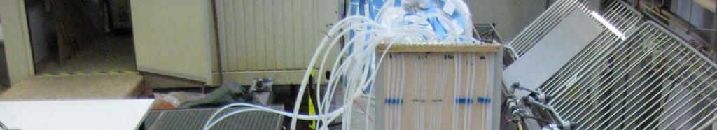
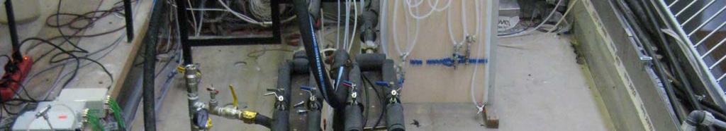
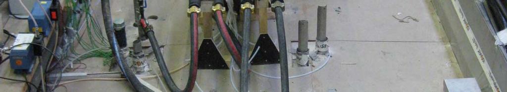
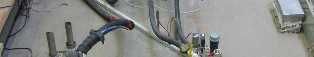
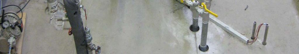
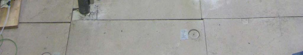
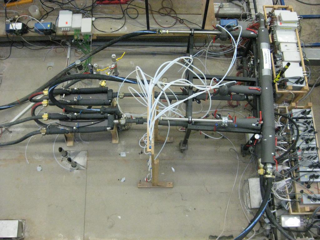
41 3.3 Technical Installations 29 Activated Carbon Filter H r ge an ch x te ea Compressor Temperature Recording GC-PID Tank Distribution and Measurement System Pressure Board E1 I3 Condensate Extraction Pumps I1 I3 Steam Distribution: I1 Saturated/Unsaturated Zone E1 Steam Distribution: Distribution and Measurement System Saturated/Unsaturated Zone E2 I2 I4 Pressure Board Figure 3.6: Technical installations of the experiment

42 30 Tank Experiment 3.4 Soil Properties The tank was set up to mimic a natural aquifer with a saturated aquitard on top, followed by an unsaturated zone. Due to the fact that filling was realized by depositing one horizontal layer after the other, one can assume that vertical anisotropy of conductivity was caused. Leube (2008) [24] stated that the vertical hydraulic permeability is reduced by a factor of 5-20 compared to the horizontal hydraulic permeability. All of the three zones, aquifer, aquitard and unsaturated zone have a thickness of 1.5 m. The aquifer zone and the unsaturated zone consist of the soil called site 3, whereas the inbetween aquitard zone is a mixture of different sands labelled M2. The mixture M2 is a composition of 24% GEBA, 16% Dorsilit , 40% Dorsilit 4900 and 20% Dorsilit to gain a sand mixture with a very low permeability. To avoid eluviation of fine material into the coarser zones, two layers with a height of about 10 cm consisting of the sand GEBA separate the M2 layer from the site 3 layers. The following Table 3.3 gives an overview over the physical parameters of the embedded materials determined by Hiester & Baker (2009) [19]. Table 3.3: Physical parameters of used materials Soil Bulk density Porosity Hydraulic conductivity Specific heat capacity ρ Bulk φ k f c p [ kg ] m 3 [-] [ m] s [ J kgk site M GEBA Observations during the experiment and analysis of simulation results suggested a better hydraulic conductivity k f of the M2 soil than measured by Hiester & Baker (2009) [19]. Guidry (2010) [15] determined the horizontal hydraulic conductivity of M2 via Darcy s equation in the flume experiment to about k f = m s. As a result of the significance of hydraulic conductivity concerning heat distribution, a better permeability would result in a faster heat distribution. In Section of the simulation results, the influence of changes in permeability was investigated by means of simulation runs with altered intrinsic permeability. Grain size distribution of site 3 soil, mixture M2 and the component sands of M2 are given in the Figures 3.7 and Dorsilit is trademark of Dorfner Group, Hirschen, Germany

43 3.4 Soil Properties 31 Sand Sieved Fraction Gravel Stone 100% Fine Medium Coarse Fine Medium Coarse 90% 80% 70% passed (%) 60% 50% 40% 30% 20% 10% 0% Grain Size [mm] Figure 3.7: Grain size distribution of site3 Elutriated Fraction Sieved Fraction 100% Clay Silt Sand Fine Medium Coarse Fine Medium Coarse 90% 80% 70% passed [%] 60% 50% 40% 30% 20% GEBA % Mixture M2 (24/16/40/20) 0% Grain Size [mm] Figure 3.8: Grain size distribution of M2 and its components

44 32 Tank Experiment 3.5 Preliminary Investigations Prior to the realization of experiments, possible physical limitations and technical expertise have to be taken into account. Furthermore, this section contains the energy balance equations used to evaluate the results of the experiment Former Experimental Investigation The tank was set up to conduct various in situ remediation experiments. Prior to the steam drive remediation approach, Leube (2009) [24] conducted soil remediation experiments using electrically driven heating elements in order to heat up the subsoil and extract the contaminants. During the experiment a total mass of 20 kg of PCE was injected into the low permeable M2 layer at two different heights (zone of interest (3.2)). The experiment concluded with a total removal of PCE 56.4%, hence, a remaining amount of about 8.72 kg in the tank. The concentration in the groundwater outflow was determined to 7.1 mg l. Measurement of PCE concentrations in the saturated zone of the tank at the end of the experiment showed a deposition of the contaminant on the side of the groundwater outflow (Fig. 3.9). PCE concentrations exceeding 100 mg m 3 were measured at a height of one meter above the ground in the saturated zone. Figure 3.9: PCE concentrations of the saturated zone, taken from Leube (2008) [24] This can be explained by contaminant transport with the condensation front towards the walls, which resulted in the displacement of PCE towards the margins of the tank. In addition, it is assumed that the contaminant gravitated partly from the original target zone within the low permeable layer into the saturated zone (aquifer). During 880 days after accomplishing the experiment, pump and treat technique was applied and achieved further contaminant removal. A mass balance considering groundwater

45 3.5 Preliminary Investigations 33 outflow samples and a groundwater flow rate of 30 l yield 2.13 kg of additional contaminant removal. The estimated contaminant mass at the beginning of this experiment h was 6.6 kg Steam Injection Pressure Injection of steam into a saturated porous medium causes a displacement of water. Considering this, it becomes clear that a certain pressure is necessary in order to displace the water from the pores. The pressure p w depends on the hydrostatic head above the injection screen of the well. However, it is of top priority not to exceed the maximum injection pressure to avoid shear failure and fractures in the subsurface where flow is preferred. Maximum injection pressure p inj is calculated as follows: p inj = p w + j p sj = ρ w gh w + i=1 j ρ sj gz j, j number of soils. (3.1) i=1 ρ w is the density of water, h w the hydrostatic head above the injection, ρ s the soil bulk density and z the thickness of the respective soil layer. Assuming the lower limit of the maximum injection pressure at the top of the well screen, the parameters yield to ρ w = kg, h m 3 w = 1.95 m, z site3 = 1.65 m, z GEBA = 0.2 m and z M2 = 1.5 m. Bulk densities of the soil materials are given in Table 3.3. Minimum injection pressure for this configuration so that steam is able to displace the water yields p w = 1.19 bar. The maximum injection pressure is determined to p inj = 1.73 bar Energy Balance Calculations The total amount of energy input is provided by the released energy during condensation ( h v ) plus the enthalpy of water at 100 C (condensed steam), cf. Trötschler et al. (2003) [32] Q in = m SI ( h v + c p,w (T x T init )) (3.2) The individual energy output of the component SVE is determined following Equation (3.3) written as Q out,1 = m SV E (h w (T ) x w + h a (T ) x a ) (3.3) where m SV E denotes the total mass of the extracted soil vapour and the enthalpy of SVE is composed of the enthalpy of air and water at the respective temperature. h w includes in addition the enthalpy of vaporization h v. The energy content of the groundwater inflow and outflow as well as the condensate extraction from the unsaturated zone is determined following Q out,2 = (m GW out c p,w T GW out m GW in c p,w T GW in ) + m C UZ c p,w T C UZ, (3.4)

46 34 Tank Experiment where c p,w denotes the specific heat capacity of water. A certain part of the energy input caused by the steam injection is stored and distributed within the system. The remaining percentage is reckoned among the energy output comprising the soil vapour extraction, the groundwater and condensate outflow and the energy losses via the tank walls. The stored energy within the system at a specific point in time can be determined following the Equations (3.5), (3.6) and (3.7). Consisting of the energy stored in the solid matrix Q s, in the groundwater of the aquifer and the aquitard Q gw and in the pore water of the vadose zone Q pw. Q s = i c p,s (1 Φ) ρ s V i (T x T init ) (3.5) Q gw = i c p,w Φ ρ w V i (T x T init ) (3.6) Q pw = i c w,s Φ ρ w V i (T x T init ) (3.7) Where c p denotes the specific heat capacity of the soil and water (c p,w = 4.2 kj kgk ), the respective porosity φ, the density ρ, the volume V i and the temperatures at initial state T init and at the considered point in time T x.

47 3.6 Slugtest Slugtest Hydraulic permeability or transmissivity, respectively, of aquifers is an important parameter for hydrogeologists to calculate flow and transport processes in the aquifer. Different methods for confined (Cooper et al. (1967) [12]) and unconfined (Bouwer and Rice (1976) [9]) aquifers are available in order to gain parameters of the aquifer. One common method is the slug test, in which water is suddenly removed from or poured into the well to observe the hereby caused rise or fall, respectively, of the water level to its initial state over time. The measured data can then be used to determine hydraulic permeability or transmissivity of the aquifer. For further information on slug test and its realization, cf. Kruseman and de Ridder (2000) [23]. As soil parameters of site 3 soil are available, a slug test would not be necessary to describe the hydraulic system. It was used to evaluate the hydraulic connection of the wells to the aquifer. Hence, slug tests were conducted for the steam injection wells I1 and I2 applying the method of Hvorslev for a confined aquifer. Performing the slug test, water level in the well is suddenly increased and the rate of descent of the waterlevel (h) is measured. The measured data of the slugtest is listed in the appendix (Ch. B) Hvorslev developed various equations to meet certain conditions, the most commonly used is Equation (3.8): k f = r2 ln ( ) L R (3.8) 2Lt 0 where k f is the hydraulic conductivity [ m ], R the radius of the screen (i.e. effective s radius), r the well casing radius and L the screen length in meters. t 0 is the time it takes the water level to fall to 37% of the initial maximum H 0. The amount of water which was poured into the well can be determined following V = (H H 0 )πr 2, (3.9) where H is the static head. The equation can be applied for any case where L R > 8. The normalized head H h H H 0 on the ordinate in log scale versus the linear scale time should yield a straight line for the recovery development with the exception of the initial lowering and the very late phase where head differences become difficult to measure. H h denotes the drawdown and H H 0 the initial water level difference. Figure 3.10 show the plots for the steam injection wells I1 and I2.

48 36 Tank Experiment 0 Recovery Development - I1 0 Recovery Development - I log [(H-h)/(H-Ho)] log [(H-h)/(H-Ho)] Time [s] (H-h)/(H-Ho) Linear ((H-h)/(H-Ho)) Time [s] (H-h)/(H-Ho) Linear ((H-h)/(H-Ho)) Figure 3.10: Normalized head over time for injection well I1 and I2 The hydraulic conductivities at the steam injection wells I1 and I2 were determined to m and m, respectively, following the method introduced in s s this section. Comparing the determined hydraulic conductivities to the hydraulic conductivity of the soil site 3 (k f = ) determined by Hiester & Baker (2009) [19], a decline in permeability of almost a magnitude is observed. This might result from compression of the porous medium at the well or clogging of the filter screen during the piling of the wells. The hydraulic conductivity of the unsaturated zone at the extraction wells E1 and E2 can be calculated using the Dupuit-Thiem well formula. Q = Kk r2πl p η ln ( ), (3.10) R r where K is the permeability [m 2 ], k r the relative permeability [-], l the filter screen length [m], p the extraction pressure [bar], η the dynamic viscosity [P a s], R the range of the well and r the well radius [m]. Taking account of the extraction pressure and the mass flow observed during cold soil vapour extraction yield a hydraulic conductivity of m and 4.8 s 10 4 m at well E1 and E2, respectively. s

49 3.7 Experimental Procedure Experimental Procedure Operating Phases Remediation with steam injection has to be considered a process with high variability. The occurrence and overlapping of processes, e.g. the breakthrough of steam at the soil vapour extraction wells requires a constant observation and adjustment of quantities. As a result of this, the remediation experiment is divided into six operation phases concerning significant changes of quantities. Table 3.4: Operating phases Phase Duration Characteristic Purpose I 42 0 d cold soil vapour extraction (medium extraction rate) and high groundwater inflow II d high steam injection rate into saturated zone (I1 and I2 ) and medium groundwater inflow III d high soil vapour extraction rate by reason of steam breakthrough at extraction wells and medium steam injection rate (I1 and I2 ) IV d low steam injection into saturated zone (I1 and I2 ) and unsaturated zone (I3 and I4 ) V d medium steam injection into saturated zone (I1 and I2 ) and shut down of steam injection into unsaturated zone (I3 and I4 ) VI d shut down of steam injection and continuous soil vapour extraction background processes enhanced remediation and steam breakthrough upkeep of thermal steady state and continuous heating of low permeable zone sandwich heating to accelerate heating plateau temperature steam override to expand steamed zone again cooling phase and capture of contaminant rebound The operating conditions applied during the individual phases are listed in Table 3.5. However, the values given herein are averaged per phase for better visualization. The accurate parameter trends of the experiment procedure are shown in the Charts 3.11 to 3.14 in this section.

50 38 Tank Experiment Table 3.5: Flow rates of operating phases Parameter Value Unit I II III IV V VI Groundwater level [m] Groundwater inflow rate [ m3 d SVE - E [ kg h SVE - E [ kg h SI - I [ kg h SI - I [ kg h SI - I [ kg h SI - I [ kg h Total energy si [kw ] Sampling and Parameter Data Acquisition Strategy The performance of experiments requires an efficient strategy concerning sampling and parameter acquisition. The acquired data is utilized to determine the experimental progress and for basic calculations. In order to be able to determine the total recovered contaminant mass subsequent to the experiment, every contaminant discharge path has to be considered. The to-be-considered paths in the conducted experiment consisted of the soil vapour, the condensate, the groundwater outflow and the condensate extraction. The observation of heat distribution requires the measurement of temperatures. Therefore, the measuring devices (Sec. 3.2) of the experiment worked automatically, recording temperatures of the tank and the contaminant concentration in the extracted soil vapour. The intervals of the collection of temperature data and the contaminant concentration were about 15 and 30 minutes, respectively. Data required to define energy and flow rate of steam injection, groundwater and soil vapour extraction was collected twice a day. Finally, chemical analysis of the discharged groundwater and the condensate/extraction well discharge was conducted twice a week by the chemical laboratory of the VEGAS to determine contaminant concentrations. The data for the determination of mass and energy flow was evaluated twice a day and the heat distribution was visualized once a day.

51 3.8 Experimental Results Experimental Results In this section, I will discuss the essential parameters of the remediation experiment. These are the mass flow (Sec ) of steam injection, soil vapour extraction and groundwater, the heat distribution (Sec ) caused by the injected steam and the thereby induced contaminant recovery (Sec ) Mass Flow The operating phases introduced in Section are the main sections of the experimental procedure and the occurring processes are discussed in detail in the following. Phase I After flooding the tank with carbon dioxide to achieve displacement of trapped air within the porous medium, start of phase I (t = 42 d) was initialized. The activation of groundwater containment with a corresponding inflow of 80 l resulted h in a piezometric head difference between the groundwater inlet and outlet of about 18 centimeters corresponding to an average water level of 3.08 m (Tab. 3.5). The aim of the application of cold soil vapour extraction (m SV E = 33 kg ) was to dewater the h unsaturated zone and stabilize the capillary fringe above the water level. As a result of the surface sealing at the top of the tank, contaminant in the unsaturated zone was extracted instantly after starting the SVE. This is visualized in Figure 3.21 as the first peak of the SVE curve. Due to problems concerning the measuring of the contaminant in the gas phase a shutdown of the soil vapour extraction was inevitable. After six days, SVE was reactivated and a continuous measuring of the contaminant in the gas phase was launched. At t = 33.8 d and t = 27 d first tests of steam injection with a flow rate of 25 and 20 kg, respectively, were conducted and resulted in new installations of h steam injection wells for reasons of poor hydraulic connection to the aquifer, cf. the slugtest (Sec. 3.6). The effect of these tests was the increase of temperature within the tank to about 24 C (Fig. 3.16) and a short-term rise of contaminant discharge in the soil vapour extraction (Fig 3.21). Phase II Phase II (t = 0d) characterizes the start of steam injection into saturated zone via injection wells I1 and I2 and a total injection rate of approximately 50 kg. Simultaneously to the start of the steam injection, the groundwater inflow was reduced from h 100 to 50 l m3 (1.2 ) which was then kept constant during the ongoing experiment. In h d general, groundwater flow serves not only as a possibility to control the flow of heat

52 40 Tank Experiment Steam Injection [kg/h] I1 [kg/h] I2 [kg/h] I3 [kg/h] I4 [kg/h] Total SI [kg/h] Soil Vapor Extraction [kg/h] I II III IV V E1 [kg/h] E2 [kg/h] Total SVE [kg/h] Time [d] Figure 3.11: Flow rates of steam injection and soil vapour extraction Flow [l/h] GWin[l/h] FLS1 [l/h] GWout [l/h] Temperatures [ C] E1[ C] E2 [ C] GWin [ C] GWout [ C] Flow [kg/h] E1 [kg/h] E2 [kg/h] I II III IV V Time [d] Figure 3.12: Flow rates and temperature of soil vapour extraction and groundwater

53 3.8 Experimental Results 41 but also to recover the aqueous solubilized contaminants. A reduction of groundwater inflow decreases the cooling effect and thereby increase the heat distribution. The applied groundwater containment system is commonly used to gain hydraulic control of contaminant plumes, discussed in Section The unsteadiness of the injection rate at the beginning (day 1 to 4) was caused by breakdowns of the steam generator. Figure 3.11 shows plots of steam injection and soil vapour extraction rates over time. When steam entered the aquifer, the extending steam bubble caused a displacement of groundwater within the porous medium resulting in a rise of groundwater outflow. This effect is visualized by the peak of the groundwater outflow in Figure 3.12 (upper graph). Along with the beginning of steam injection, a steep climb of the groundwater outflow temperature (Fig. 3.12, lower graph) as condensing steam transfered heat to the passing groundwater flow was observed. The lowering of the groundwater inflow temperature had origin in the switching of previous used groundwater cycle to now fresh water supply by the degasing installation. After four days of steam injection a significant increase of the soil vapour extraction temperature suggested the beginning of steam breakthrough at the extraction wells E1 and E2 (Fig. 3.11, lower graph). The significant reduction of the steam injection rate from 52 to 40 kg was to prevent steam from climbing at the long sides h of the tank and the therein resulting endangering of the pneumatic containment. By reason of the requirement of pneumatic containment, modifications were applied to the soil vapour extraction equipment in order to provide an increase of the extraction rate. A significant rise of the total extraction rate from 30 to 65 kg (Fig. 3.11) yielded h finally the steam breakthrough and led to the increase of energy output of the SVE to 3.75 kw, marking the start of phase III. This is visualized in Figure 3.26 (energy balance). Phase III The self-adjusted higher extraction flow rate at E2 (from t = 8.8 d forward) indicates a better connection of the well to the vadose zone or a better hydraulic conductivity, respectively. The difference of these flow rates was kept in order to capture the preferred vertical pathway of the steam propagation on the side of the extraction well E2 of the tank. The established pneumatic capture reduced the problems of steam breakthrough after three days (t = 11.1 d). Then the steam rate was increased to around and held constant during the rest of the phase. The renewed increase of steam injection resulted in a new displacement of groundwater, indicated by the raise of the groundwater outflow in Figure Accompanying the increased extraction rate and the steam breakthrough is the rising of the outflow of FLS1 as shown in Figure kg h

54 42 Tank Experiment Flow [kg/h] Flow [l/h] I1 [kg/h] I2 [kg/h] I3 [kg/h] I4 [kg/h] Flow [kg/h] E1 [kg/h] E2 [kg/h] I II III IV V GWin [l/h] FLS1 [l/h] GWout [l/h] Time [d] Figure 3.13: Flow rates of steam injection, soil vapour extraction, groundwater and condensate tank Flow Rate [m³/d] I II III IV V 70 Temperature [ C] Time [d] GW Inflow GW Outflow Figure 3.14: Flow rates and temperature of groundwater

55 3.8 Experimental Results 43 In addition, the condensate extraction from the unsaturated zone, collected as well in FLS1, increased the outflow rate. The amount of water is composed on the one hand by condensed steam and on the other by water pushed from the lower to the upper zones as a result of the applied pressure from the steam injection. By means of Darcys law, the upward flux in the center of the tank is determined by taking into account the pressure gradient p = h. The pressure head difference of about m between 1.8 y l and 2.6 meters above ground level resulted in a flux calculated to 0.76 at steady h m 2 state at the end of phase III (t = d). Phase IV The achievement of a steady state condition concerning vertical heat distribution induced the beginning of phase IV, which was characterized by the investigation of effects of additional steam injection into the unsaturated zone via the injection wells I3 and I4. Contrary to the initial expectations, the injection of steam only into the saturated zone achieved a temperature increase to about 90 C at the top of the low permeable M2 layer in the center of the tank. At t = 28.8 d a total steam injection and a corresponding energy input of about 9 kw caused a reduction of steam injection rate in the saturated zone to 36 kg h (23 kw ). A simultaneous increase of the energy output via soil vapour extraction from previous 3.7 to around 8.5 kw was observed, indicating a fast steam breakthrough in the unsaturated zone (Fig. 3.26). flow rate in the unsaturated zone of about 12 kg h Comparing steam injection rates and groundwater outflow in Figure 3.13, one can observe a decrease of the groundwater outflow resulting from the collapse of the steam bubble in the saturated zone wich was induced by the reduction of the steam flow rate (t = 28.8 d). After two days from the start of the unsaturated steam injection, one observes an increase of the outflow rate and the energy output of the FLS1, cf. Figure 3.13 and The close distance of the injection wells I3 and I4 to the extraction wells E1 and E2, respectively, as well as the instantaneous rise of the SVE energy output indicated a limited expansion of heat in the unsaturated zone as the main part of the energy input left directly via the SVE. According to this thermal shortcut and since no further significant change in heat distribution in the unsaturated zone was observed, the injection into the unsaturated zone was shut down after 13 days (t = 44.9 d) of operation. Furthermore, no significant rise in the contaminant discharge via SVE during the steam injection into the unsaturated zone was observed and confirmed the complete remediation of the unsaturated zone. In addition, the contaminant discharge in the groundwater outflow stagnated at the end of phase III at an unsatisfactory concentration of approximately 700 mg, cf. Figure This reinforced the assumption of subsidence of contaminant from its original location within the low permeable m 3 M2 layer into the aquifer (saturated zone) and required further remediation of the saturated zone.

56 44 Tank Experiment Phase V Since neither mass extraction nor heat distribution was enhanced by the steam sandwich technique, the reinitiating of steam injection only into the saturated zone in order to achieve further contaminant recovery from the saturated zone was startet. The steam injection flow rate was increased from 38 to 47 kg (35 kw ) in order to re-expand the h steamed zone in the aquifer which resulted again in the displacement of groundwater (Fig. 3.13) and temperature increase (Fig. 3.14). Phase VI After 14 days, at t = 64 d, the steam injection was shut down and the cold soil vapour extraction was maintained in operation for another two days in order to capture the contaminant concentration rebound. An increase of the SVE flow rate after the shutdown of the steam injection was observed. This can be explained by the reduced amount of steam in the SVE which reduced the viscosity and caused an increase of relative permeability as the temperature of the soil vapour decreased. The remediation experiment was terminated after 65.8 days.

57 3.8 Experimental Results Heat Distribution Heat distribution is the main concern of a thermally enhanced in-situ soil remediation. This section discusses the distribution observed during the different phases of the remediation experiment, shown in Figure 3.16 and The plots were drawn by means of Tecplot TM (Tecplot, Inc., Bellevue, USA) from the acquired temperature data at the two cross-sections (Fig. 3.1). The temperature plots show the three-dimensional view of the tank with six horizontal planes at different heights and one vertical plane in the center of the tank. As there are only these two cross-sections, temperature profiles H to A were mirrored at profile J to the other side of the tank to improve the visualization of the heat propagation in the tank. Furthermore, the measured groundwater inflow and outflow temperatures were set at the location of the horizontal groundwater inflow and outflow well, respectively. Groundwater inflow is located at the right hand side and outflow on the left hand side, respectively. The temperature ranges from 20 to 100 C. The vertical black lines represent the location of the steam injection wells I1, I2, I3 and I4 as well as the extraction wells E1 and E2. The initial temperature within the tank at the beginning of phase II was measured to be 24 C (Fig 3.16). Figure 3.15 shows the averaged temperature of the saturated zone (0 y 1.5 m), the low permeable M2 zone (1.5 y 3 m) and the unsaturated zone ( m) from t = 0 d. 100 I II III IV V Temperature [ C] Time [d] Saturated Zone Low Permeable M2 Zone Unsaturated Zone Figure 3.15: Temperature trends of saturated, low permeable M2 and unsaturated zone

58 46 Tank Experiment Figure 3.16: Heat distribution plots of remediation experiment (1 18d)

59 3.8 Experimental Results 47 After one day of steam injection, a horizontal distribution was observed as the ascent of the steam caused by buoyancy effects was hindered by the presence of the low permeable M2 layer. Furthermore, a slight warming alongside the injection wells caused by heat conduction was observed. The steam front reached the long sides of the tank at t = 4 d establishing an expanded steamed zone below the aquitard layer. At t = 8 d, one can observe the consequence of the steam override process below the low permeable layer, heating the latter. As a result of the heated aquifer, groundwater inflow at a temperature of about 18.5 C is visible demonstrating the cooling effect on the heating process. As a consequence of the high steam injection rate and therewith a relative high injection pressure, a fast ascending of the steam at the long sides of the tank was observed. In order to prevent this effect, the steam injection rate was reduced significantly while the soil vapour extraction rate was increased at t = 8.8 d, illustrated in Figure 3.11 (Phase II). Temperature plots at t = d illustrate the continuous heating process of the low permeable M2 layer over the almost entire ground area. After 28 days of steam injection into the saturated zone with a total energy input of about 22 kw h, steady state was reached concerning the heat distribution. The corresponding plot demonstrates the successful warming-up of the low permeable layer up to the top at H = 3 m above ground level, exceeding the temperature of 90 C. However, this region was constricted to the area between the injection wells I1 and I2 which was in fact the original target zone where the contaminant had been infiltrated in The combined steam injection into the saturated and the unsaturated zone (steam sandwich) at the beginning of phase IV (t abs = 28.8 d) demonstrated a significant effect on the heat distribution (Fig. 3.17). Comparing the temperature plots after 28 and 31 days of steam injection, a clear decrease of the steam front expansion in the aquifer at a height of about 0 H 0.7 m was observed, which came along with an expansion of the cold groundwater inflow region. Furthermore, an increase of temperature in the vadose zone above the low permeable layer at the injection wells I3 and I4 was detected. At t = 38 d, after 9 days of combined steam injection, no further temperature expansion in the vadose zone was noticeable as a result of the close distance to the soil vapour extraction wells. Hence, the steam flow rate into the unsaturated zone was reduced from this point in time until such time as the complete shut-down of the steam injection into the unsaturated zone at t = d. In order to achieve again a wide-spread expansion of the steam front in the aquifer, the steam injection rate into the saturated zone was increased once again (phase V). At the end of the steam injection at t = 64 d no further heat expansion was noticeable.

60 48 Tank Experiment Figure 3.17: Heat distribution plots of remediation experiment (28 63d)

61 3.8 Experimental Results 49 Figure 3.18 shows the temperature trend of selected temperature sensors of the profile J in the center of the tank at 1.55 (bottom of M2 ), 2.25 (middle of M2 ), 2.95 (top of M2 ) and 3.30 m (unsaturated zone) above ground level. Observing a strong rise of temperature in phase II at each sensor, then was reduced during phase III. Due to buoyancy forces effecting vertical steam propagation the temperature at H = 1.55 m, at the bottom side of the low permeable M2 layer, reached 100 C after the first day of steam injection. The abrupt temperature fall was a result of the short-time steam generator breakdown. In the center of the aquitard (H = 2.25 m), a constant temperature of about C was reached at the end of phase II. At t = 15.9 d, the zone of interest (J-295 ) was heated to the target temperature of about 90 C. At the end of phase III, J-295 at the top of the aquitard displayed a temperature at this point in time of about 99.6 C at H = 2.95 m and and 79.4 C at H = 3.30 m. The combined steam injection only affected the temperature in the vadose zone, cf. J-330, showing a significant rise at the beginning of phase IV and an instantaneous temperature decrease caused by the shut-down of the injection wells I3 and I4. However, the J-330 reached a maximum temperature of 90.6 C although steam was injected into the unsaturated zone. The closer distance of the injection wells I3 and I4 to the extraction wells E1 and E2, respectively, than to the temperature sensor J-330 was responsible for this behaviour. 110 I II III IV V Temperature [ C] Time [d] J-155 J-225 J-295 J-330 Figure 3.18: Temperature trends of profile J temperature sensors In Section 2.9 the typical behaviour of steam propagation in saturated zones was discussed. Figure 3.19 depicts the impact of buoyancy forces on the injected steam observed after three and 28 days of steam injection. The heat distribution plot is illus-

62 50 Tank Experiment trating the cross-section in the center of the tank. Contaminants are transported with the condensation front ahead of the steam front. Hence, fractions of the contaminant in the saturated zone were pushed to the margins of the tank and deposited there as the steam could not propagate further to the walls. The two ellipses mark the location of the potential contaminant deposition. Figure 3.19: Effect of buoyancy forces on steam propagation (t = 3 & 28 d)

63 3.8 Experimental Results Contaminant Recovery The energy input by steam injection in the tank enhanced significantly the recovery of contaminant (PCE). After 65.8 days of remediation, a total amount of about 3.03 kg was removed from the subsoil in the tank. This matches 45.8% of the initial total amount previously estimated (Sec. 3.5). Chart 3.20 depicts the percentage of the individual discharge path concerning the total contaminant recovery sum. 88% 1% 11% Soil Vapour Extraction Groundwater Condensate - Unsaturated Zone Figure 3.20: Percentage distribution of contaminant recovery The main discharge path was the soil vapour extraction with a removal of 2.68 kg (88%). The groundwater outflow removed 0.33 kg (11%) kg (1%) of the contaminant was extracted with the condensate from the unsaturated zone. The relation between the recovered contaminant and the steam energy input yielded a thermal effort of about 17.2 MW h, which corresponds to 1440 e, per recovered kilogram of contaminant. A pump and treat technique would need about six years with a flow rate of Q = 30 l (energy consumption: 300W ) to remove 3 kg of contaminant h from the tank. The energy effort would be MW h (1114 e) per kilogram of contaminant. Figure 3.21 depicts the contaminant removal in unit mass per unit time of the SVE and the GW as well as the total sum of the recovered contaminant amount. Figure 3.23 and 3.22 show PCE concentrations of the SVE and the groundwater outflow as well as the groundwater outflow and the FLS1, respectively. Furthermore, the cumulative sums of the contaminant of the individual contaminant recovery paths are shown in Figure 3.24.

64 52 Tank Experiment At the beginning of the experiment, an initial concentration of PCE of about 1.8 mg was measured in the groundwater outflow (Fig. 3.22). Preliminary to the l start of the steam injection (phase II), the extracted soil vapour measured no PCE concentrations. The steam injection tests during phase I (cf. Sec ), however, caused concentration peaks in the extracted soil vapour for a short time. The increase of contaminant removal in the groundwater outflow may be related to the steam tests. Simultaneous to the start of the remediation experiment (t = 0 d), a significant rise of the contaminant removal in the groundwater was observed (Fig. 3.21). The input of heat into the porous medium provoked a fast recovery at the already heated area around the injection wells. The fast recovery was caused by the better solubility of PCE in water and the reduced residual saturation of PCE due to the increased temperature. This effect benefited the drift of PCE, which was induced by the groundwater flow. As a result of this, the maximum concentration measured in the groundwater outflow was about 3.29 mg (Fig. 3.22, t = 2.8 d). The peak in l Figure 3.21 demonstrates the importance of the groundwater containment system (GCS) concerning contaminant removal and protection of downstream located areas. The GCS not only provided a possibility to control contaminant plumes but also represented a minor remediation path (max. 11%). After 2.8 days of steam injection, the concentration of PCE in the gas phase of the SVE began to rise observably to the highest discharge rate of about 240 g d at t = 8.5 d. With the increase of the soil vapour extraction rate at the steam breakthrough (t = 4 d), a simultaneous removal rise of FLS1 with a maximum discharge concentration of about 2.4 g after 8.8 days from the beginning of SI was d observed. By theory, the recovered contaminant mass in FLS1 was extracted by the SVE and removed during offgas treatment. Within phase III, the comparative constant effective energy input (Fig. 3.26) characterized a decline concerning the contaminant discharge rate in every discharge path. Comparing Figure 3.23 from t = 28.8 d on, the additional steam injection into the unsaturated zone (steam sandwich) caused no supplemental contaminant recovery. This confirmed the assumption that contaminants gravitated from its original location within the M2 layer towards the bottom of the tank since the performance of the previous remediation experiment in The shut-down of the unsaturated steam injection wells at the beginning of phase V and the increase of the steam flow rate into the saturated zone resulted again in an increase of contaminant discharge concentration in the SVE and the groundwater outflow (Fig. 3.22). Finally, at t = 64 d, the contaminant concentration of SVE, groundwater outflow and FLS1 stagnated at around c SVE = 9.5 mg, m 3 c GWout = 360 mg and c m 3 FLS1 = 110 mg. The steam injection was therefore ceased. The m 3 shut down induced a high vacuum in the steamed zone, which mobilized additionally previous trapped contaminant. Thus, a concentration rise in the extracted soil

65 3.8 Experimental Results 53 vapour could be observed reaching a maximum value of about 50 mg. Along with m 3 the increase of concentration in the extracted soil vapour, a raised concentration in the outflow of the FLS1 was observed (Fig. 3.23). After two days of cold soil vapour extraction, the contaminant concentration in the soil vapour decreased to 0.5 mg and indicated the end of the remediation and the termination of the experiment. m 3 The steam injection was responsible for the significant increase of the contaminant removal (Fig. 3.22). The contaminant concentration in the groundwater decreased by 85% compared to the initial contaminant concentration. However, compared with the SVE (99%), the relative contaminant removal remained at a comparative high value. The persisting contamination of the saturated zone is evident. The aqueous equilibrium concentration of the measured SVE concentrations can be determined by means of Henry coefficient of PCE. The dimensionless Henry coefficient at 20 C (gas temperature at the heat exchanger outflow) is H = (EPA Site Assessment Calculation Tool [2]). The calculated aqueous concentration in comparison with the measured concentrations of the FLS1 showed a significant discrepancy, cf. appendix (A.2). Contaminant concentrations of the FLS1 were 10 to 40-fold higher. Although condensate was removed from the unsaturated zone, it is possible that fractions of condensed contaminant accumulated there as steam propagation was limited in the unsaturated zone. This expressed the need for condensate extraction from the unsaturated zone.

66 54 Tank Experiment I II III IV V Mass Flux of PCE [g/d] Total Recovery of Contaminant [kg] Time [d] Total Recovery [kg] SVE [g/d] Groundwater [g/d ] C-UZ [g/d] Figure 3.21: Contaminant discharge rate and total sum 4000 I II III IV V 3500 Contaminant Concentration [mg/m³] Time [d] Groundwater [mg/m³] FLS1 (Condensate) [mg/m³] Figure 3.22: Contaminant concentration of groundwater and condensate tank

67 3.8 Experimental Results I II III IV V Concentration in GW [mg/m³] Concentration in SVE [mg/m³] Time [d] Groundwater [mg/m³] SVE [mg/m³] Figure 3.23: Contaminant concentration of soil vapour extraction and groundwater 3.5 I II III IV V Individual Contaminant Recovery [kg] Total Contaminant Recovery [kg] Time [d] SVE [kg] Groundwater [kg] C-UZ Total Recovery [kg] Figure 3.24: Cumulative contaminant recovery

68 56 Tank Experiment Water Mass Balance The remediation experiment using steam injection technique was dominated by significant water flows compared to the air flow. Not only the groundwater flow but also the steam injection and the soil vapour extraction caused a water mass flow. In order to be able to quantify the water displacement by the injected steam and determine the amount of condensed steam, the water mass balance for the tank (saturated and unsaturated zone) was determined considering the relevant quantities. The total amount of water in the tank at t = 0 d can be determined by means of the geometry of the tank, the porosity of the soils and the initial water level or water saturation, respectively. Full saturation in the aquifer and the aquitard as well as in the two transition layers below and above of it was assumed. The water saturation of the vadose zone was estimated to S V Z = During steam injection water was displaced from the tank caused by the expanding steam zone. The water displacement is calculated from the difference between the input and output water mass. The amount of condensed steam in the tank is defined as the difference between steam mass and soil vapour condensate. Table 3.6 contains the water mass balance of phase II-III and II-IV as well as the total mass balance after the termination of the remediation experiment. At the end of phase III and IV, respectively, approximately 90% of the injected steam condensed in the tank. 20% of the water in the pore volume was replaced by the steam at the end of phase III and 7% at the end of phase IV.

69 3.8 Experimental Results 57 Table 3.6: Mass balance of remediation experiment (phase II-III, II-IV & total) Phase II-III II-IV Total Unit Container specifications Duration d Volume of tank 81 m 3 Pore volume m 3 Initial water content kg Remaining water content kg Removed water percentage % Total mass Steam kg Groundwater inflow kg Groundwater outflow kg Condensate kg Extraction well d/c kg Displaced water kg Condensed steam in soil kg Ratio (displaced water / injected steam) %

70 58 Tank Experiment Energy Balance The application of steam injection into the saturated and unsaturated zone was successfully accomplished concerning the main objective of heating the top of the aquitard up to 90 C (Sec ). Comparing the experiment charts and the temperature plots, it is evident that the energy input of the injected steam and the energy output show a highly interdependent behaviour during the entire experimental procedure. Hence, Figure 3.25 visualizes the input and output quantities in a schematic sketch, derived from Trötschler et al. (2004) [32]. Steam Injection QSI Groundwater Inflow QGWin Container Groundwater Outflow QGWout Energy Losses QL Condensate Extraction QC-UZ Soil Vapour Extraction QSVE Figure 3.25: Energy input and output quantities The thermal energy input includes the steam injection Q SI and the groundwater inflow Q GW in. The extraction of soil vapour Q SV E and the groundwater outflow Q GW out contribute to the energy output. The extraction wells water discharge Q C UZ (condensate from unsaturated zone) counts in addition to the regular energy output quantities. The effective energy input is then determined by the difference between the input and output quantities and denotes the remaining energy quantity delivered to the porous medium. The outcome of the high energy input was an extensive heat expansion as far as the tank walls. Considering this, energy losses via the tank walls must not be neglected and, therefore, will be discussed in Section Figure 3.26 depicts the energy input and energy output over the duration of the remediation experiment. The effective energy input corresponds to the steam injection energy, influenced by the changes in the groundwater energy output. These changes can be traced back to the sensitivity of the steamed zone concerning even minor changes in the steam injection rate, e.g. caused by re-adjustments of the flow rate or maintenances of the steam generator.

71 3.8 Experimental Results 59 A major difference was observed in phase IV (t = 28.8 d) during combined steam injection into the saturated and unsaturated zone. In spite of an increased energy input (SI ), the effective energy input decreased slightly. This is explained by the major increase of the energy output in the soil vapour extraction and the resulting condensate. From t = 40 d on, the injection into the saturated zone was slightly increased and the flow rate into the unsaturated zone decreased as illustrated in Figure Herefrom resulted the rise of the effective energy input as a result of the drop of energy output of the SVE and the condensate (t = 39 d). 45 I II III IV V Energy [kw] Effective Power Input [kw] Time [d] Qout SVE [kw] Qin SI [kw] Eff. Power Input [kw] Qin-out GW [kw] Qout UZ-Discharge [kw] Figure 3.26: Energy input and output At the end of phase III, steady state of heat distribution was reached, cf. Section In state of equilibrium no more energy is used to heat the soil and pore water of the tank. The difference between input and output quantities represents the effective energy input which was used to heat up the tank. However, at steady state the inputoutput difference denotes the energy losses via the tank walls. Table 3.7 lists the total cumulative input and output (II-III, II-IV and Total) since start of steam injection at t = 0d and the averaged momentary energy input and output at the end of phase III (t = 28.8d).

72 60 Tank Experiment Table 3.7: Energy balance of remediation experiment (phase II-III, II-IV & total) Phase II-III II-IV Total Duration [d] Mass Energy Mass Energy Mass Energy Sum [ 10 3 kg] [MW h] [ 10 3 kg] [MW h] [ 10 3 kg] [MW h] Steam Groundwater inflow Groundwater outflow Soil vapour extraction Condensate Extraction well d/c Effective energy Flow rate [ kg h ] [kw ] Steam Groundwater inflow Groundwater outflow Soil vapour extraction Condensate Extraction well d/c Heat loss The energy stored within the porous medium of the tank can be calculated by means of Equations (3.5), (3.6) and (3.7). Therefore, the porosity and the bulk density of the soil (Tab. 3.3) and the initial temperature of about 24 C are needed. The average temperature at the end of phase III (t = d) and IV (t = d) of the steam injection of each layer was calculated by means of the program Tecplot TM and listed in Table (3.8). Taking into account the temperature difference, the total amount of the stored energy within the tank at the end of the respective phase yield Q III pm = GJ (3.37 MW h) and Q IV pm = GJ (3.4 MW h). Considering the total effective energy input of about Q eff = GJ and the stored energy at the end of phase III, yield a difference of about Q l = GJ (23.6 MW h) which is the total amount of energy losses across the system boundaries. Table (3.9) lists the amount of stored energy of the single parts within the tank and the corresponding percentage.

73 3.8 Experimental Results 61 Table 3.8: Averaged temperatures of porous medium (t = d & d) Phase III IV Layer Height [m] Temperature [ C] Vadose zone (site 3 ) 3.1 y Transition layer 1 (GEBA) 3.0 y Aquitard (M2 ) 1.5 y Transition layer 2 (GEBA) 1.4 y Aquifer (site 3 ) 0.0 y Table 3.9: Stored energy in porous medium (t = d & d) Phase III IV Part Energy Percentage Energy Percentage [GJ] [%] [GJ] [%] Soil Q s Groundwater Q gw Pore water in vz Q pw Total Q pm

74 62 Tank Experiment Tank Heat Loss Estimation In Section the horizontal expansion of the steam front extending to the walls of the tank is discussed. Hence, heat losses via the surrounding tank walls, namely the sides, the top and the bottom of the tank were determined by means of the equations given in Section 2.6. The determination of the heat losses required the separate consideration of the tank parts due to the occurrence of different processes and the set-up of the tank. Heat loss calculations are taken from VDI-Wärmeatlas (2006) [20]. Front: Free convection at vertical plate (Churchill and Chu) and radiation Nu = { [Ra f 1 (P r] 1/6 } 2 (3.11) [ ( ) ] 9/16 9/ f 1 (P r) = 1 + (3.12) P r Top: Free convection at horizontal plate (heat emission at top face) and radiation Determination of Nusselt number for laminar flow, Ra F 2 (P r) , defined by Churchill Nu m = 0.15 [Ra f 2 (P r)] 1/3 (3.13) [ ( ) ] 11/20 20/ f 2 (P r) = 1 +. (3.14) P r Bottom: Free convection at horizontal plate (emission at rear side) and radiation To determine the Nusselt number after Churchill: Nu m = 0.6[Ra f 1 (P r)] 1/5 (3.15) where f 1 (P r) can be calculated, cf. Equation (3.12) and the characteristic length is determined as l = (a b)/(2(a + b)). Back and Sides: Conduction through layers As the back and side parts of the tank are next to the other tanks, conduction through the saturated soil and the HDPE-wall, which separates the cooling gap from the porous medium has to be considered. This requires the definition of the thermal conductivity coefficient k, 1 ka = (3.16) α 1 A 1 α i A i Considering s as the wall thickness in meter and A the reference area in square meter. α i is calculated, following α i = λ i s i. (3.17)

75 3.8 Experimental Results 63 The heat losses are calculated for steady state conditions at t = d. Temperatures of the walls were measured randomly at different locations and postprocessed by means of Tecplot TM. The total sum of heat losses was determined to 22.3 kw due to the global energy balance of the experiment, cf. Section The heat losses of the tank can be estimated applying the introduced approaches (Tab. 3.10). Table 3.10: Heat losses at steady state (t = d) Part Conduction Radiation Convection Total [kw ] [kw ] [kw ] [kw ] Top Bottom Front Back Sides Sum % 31% 34% 8% 3% Front Top Bottom Back Sides Figure 3.27: Energy loss percentage of single tank parts The calculated total heat loss of about 22.4 kw matches the heat losses determined by the energy balance. As temperatures were extrapolated and averaged per tank wall area, the calculations can only be considered as an estimation. Figure 3.27 visualizes the percentage of the total energy loss contributed by the single parts of the tank.

76 64 Tank Experiment 3.9 Comparison of 1D Numerical Model and Experiment The observed heat distribution of the experiment was compared to the vertical temperature development simulated by a 1D numerical model. Guidry (2010) [15] set up a 1D transient model which was originally developed for heat conduction in solid media (Schneider (1955) [30]). The purpose of the model is the simulation of the heat distribution in a low permeable layer by steam override in order to determine the heating-up time and the temperature levels in the layer. The principle of the model is the subdivision of the system into a number of regular physical and geometrical volumes to consider the heat processes for one cell between the two surrounding cells. The relevant processes for the simulation of the heat propagation implemented in the model are heat convection, heat conduction and the heat loss to the environment. The change in internal energy over time is then equal to the difference between the injected heat and the heat loss. This results in a temperature increase for transient condition. A constant temperature at the bottom of the first cell and at the top of the last cell simulates the steam injection at the bottom and the temperature of the environment at the top. For detailed information it is referred to Guidry (2010) [15]. The 1D model successfully simulated the heat distribution of the flume experiment. The calculated final temperatures on different heights in the flume as well as the temperature trend over time was reproduced correctly. The model was additionally adapted to the tank in order to simulate the heat distribution observed in this experiment (Fig. 3.28). Figure 3.29 is the spreadsheet which contains the input data of the model responsible for the simulation of the heat distribution. Figure 3.28: Set-up of 1D model for the tank simulation

77 3.9 Comparison of 1D Numerical Model and Experiment 65 Figure 3.29: 1D model spreadsheet for the simulation of the tank experiment However, the model was not able to reproduce neither the maximum temperature nor the temperature trend correctly. Figure 3.30 shows the temperature trendlines of the experiment and the 1D model. The fast increase of the temperature results from the heat convection term determined by the steam injection rate. The contribution of the heat conduction term is negligible compared to the convection. This explains the temperature plateau as the convective term gets reduced after a certain time and no further temperature increase is achieved by the conduction term Temperature [ C] aquifer (m) 190 (m) 225 (m) 260 (m) 305 (m) 330 (m) 380 (m) V190 (e) V225 (e) V260 (e) V305 (e) V330 (e) V380 (e) Time [d] Figure 3.30: Comparison of temperature trendlines of 1D model and experiment

78 66 Tank Experiment The main shortcoming of this model is the non-implementation of the heat mass balance. The model is not able to determine whether steam entered a cell or not. This prevents the consideration of a decline of the heat transfer coefficient from one cell to the next. The heat transfer coefficient is responsible for the convection and, therefore, the fast heat transport. A reduction of the heat transfer coefficient by hand yielded a better approximation to the experimental curves due to the fact that heat conduction increased but also resulted in a significant decrease of the maximum temperature. The model could be successfully applied to the flume experiment due to the fact that convective processes were responsible for the heat distribution. In the tank experiment, however, the heat conductive process predominated the heating of the low permeable layer, which is responsible for the unsatisfactory applicability of the model.

79 3.10 Follow-Up Investigations Follow-Up Investigations According to Section 3.8.3, it is assumed that an amount of about 3.5 kg of PCE remained in the saturated zone of the tank. Although the emissions by groundwater were significantly reduced from 1.8 mg to 0.3 mg, further remediation is necessary to l l achieve the desired complete recovery. Due to the limitation of the continuous steam injection technique to remediate the lower parts of the saturated zone, the technique has to be adapted or changed. The following observations emphasize the demand for a remediation technique modification: a) Decline of contaminant concentration in soil vapour extraction b) Steam injection achieved no further contaminant removal c) Contaminant removal from the unsaturated zone was higher in comparison with the saturated zone d) Partitioning of contaminant in the saturated zone e) Assumption: contaminant partitioned in lower sections or boundary areas, which were unaffected by the steam Two thermally enhanced remediation options are (1) the intermitted steam injection technique and (2) the steam injection after complete drainage of the tank. The intermitted steam injection technique is derived from the cyclic steam injection which is a commonly applied technique in the petroleum industry to increase oil production (Klinginger (2010) [22]). In our case of remediation, steam is injected until the saturated zone is heated and steam breaks through at the extraction wells. The shutdown of steam injection then induces a fast increase of contaminant concentration in the extracted soil vapour, cf. Section Due to high vacuum extraction further contaminant can be removed in an energy optimized way. The drainage of the tank transforms the former saturated into an unsaturated zone. This benefits the steam propagation as buoyancy forces occurring in the saturated zone are not present. Hence, horizontal steam propagation is more wide-spread and the remediation of the former saturated zone is more efficient. As a matter of course, realization of this technique in the field is not as simple as in the experiment. However, lowering of the groundwater level can be achieved by means of sheet piling in combination with groundwater extraction wells, which then are able to extract the groundwater and the condensed steam enriched with contaminants.

80 4 Numerical Simulation This part of the thesis describes the set-up of a numerical model for simulations of steam injection into a porous medium. It is intended to reproduce the heat distribution observed during the experimental investigation (Sec. 3.7). The results of the simulation are then compared with the results from the experiment. Since the main interest lies in the heat distribution, only the aqueous and the gaseous phase are considered. These two phases consist of the components air and water. Furthermore, any nonaqueous phases/components are neglected in the simulation. Investigations on steam propagation conducted by Ochs et al. (2003) [27] illustrated that the presence of a NAPL has no significant effect on the propagation of the steam front. Further, NAPL distribution was not investigated during the experiment, which is of importance if the simulation of contaminant distribution is of interest. However, two components have to be considered because the model domain comprises the unsaturated zone in addition to the saturated zone. The consideration of only one component (water) would be conform if only saturated zones are present. According to these statements the choice was made for a non-isothermal, two-phase, two-component modeling approach (2p2cni). Figure 4.1 shows the present phase states and their corresponding relation due to mass transfer processes. Modeling steam injection into saturated zones might cause various Figure 4.1: Phase states and mass transfer processes of a 2p2cni model, taken from Ochs (2007) [28] difficulties, for example numerical instabilities if the air component is not present. For further insight related to model stability, extensive investigations on simulating steam injection into saturated zones were accomplished by Ochs (2010) [28]. 68

81 4.1 MUFTE-UG MUFTE-UG The simulations were realized by means of MUFTE-UG. MUFTE is the abbreviation for Multiphase Flow, Transport and Energy model, containing physical model concepts and discretization methods for isothermal and non-isothermal multiphasemulticomponent flow and transport processes in porous and fractured media (Helmig et al. (1998) [17]. UG stands for Unstructered Grid and comprises the data structures and solvers for the discretization of partial differential equations. MUFTE-UG was developed at the Universität Stuttgart (IWS) in co-operation with the Universität Heidelberg. The spatial discretization uses the BOX method where boxes are constructed around each node allowing fluxes to be calculated at their borders. The total flux between node i and j then is composed by the sum of all fluxes of the subcontrol volumes related to node i and j. For further insight on discretization techniques, I refer to Helmig & Huber (1998) [18]. 4.2 Primary Variables In order to describe our multiphase system a defined set of independent variables is needed, denoted as primary variables. The remaining variables, known as secondary variables, required to solve the non-linear system equations can then be derived by means of constitutive relationships such as (1) the capillary pressure constraint (Eq. 2.14) and (2) the saturation constraint (Eq. (2.6)). In Table 4.1, the different phase states with the corresponding primary variables for a 2p2cni model are listed. Table 4.1: Phase states and primary variables of the 2p2cni model Phase state Present phases Primary variables Water phase w x a w, p g, T Gas phase g x w g, p g, T Both phases w,g S w, p g, T

82 70 Numerical Simulation 4.3 Mathematical Model of a Non-Isothermal System Balance equations are used in order to describe the behaviour of fluids in a porous medium. The balance equations comprise generally mass, momentum and energy. Considering non-isothermal, two-phase, two-component systems, not only mass but also energy has to be conserved in each phase and component. On the local scale (REV ) the momentum balance is represented by the extended Darcy s law substituting the Navier-Stokes-Equation which describes flow on the pore scale. In the applied model we have to consider a gas phase consisting of air and steam and a water phase composed of water and dissolved air. In order to be able to solve the strongly coupled differential equations various simplifications such as the assumption of local thermodynamic equilibrium are used. As the explicit derivation of the Reynolds Transport Theorem and the balance equations are beyond the scope of this thesis, I refer for detailed information to Helmig (1997) [16] and Class (2001) [10] Continuity Equation According to mass conservation within a finite control volume following the continuity condition ( dm dt ) Ω = 0, one can formulate the mass balance equation for both components κ, accumulation term {}}{ advection term ( ) {}}{ φ ( ) ρ mol,α x κ kr,α t αs α ρ mol,α x κ µ αk( p α ρ mass,α g) α α α (D ) pmρ κ mol,g q κ = 0, }{{}}{{} diffusion term sink/source term (4.1) with the porosity φ and the intrinsic permeability K of the porous media, the molar density ρ mol,α and mass density ρ mass,α, the saturation S α, the pressure p α, the relative permeability k r,α and the viscosity µ α of the phase α. x κ α describes the mole fractions of the component κ in the particular phase α. q κ denotes the source/sink term and D κ pm the diffusion coefficient of component κ Energy Equation In accordance with the first law of thermodynamics, the energy of a system cannot be lost but only transferred from one state to another. Hence, a change of the system internal energy U is due to transport of energy across the borders and/or work performed by/to the system itself. In a porous medium, thermal energy is stored within the porous matrix and exchanged to and between the fluids. With the assumption of local thermal equilibrium, which is reasonable for small pores and, therewith, small velocities, the temperatures of all phases are equal within

83 4.3 Mathematical Model of a Non-Isothermal System 71 an averaging volume and, therefore, one equation for thermal energy is sufficient. accumulation term { ( }} ) { φ ρ mass,α u α S α + (1 φ) t t (ρ sc p,s T ) α conduction term {}}{ (λ pm T ) ( ) kr,α ρ mass,α h α K( p α ρ mass,α g) µ α α }{{} convection term (D ) pmρ κ mol,g h mol,g M κ x κ g q h = 0 }{{} κ }{{} sink term diffusion term (4.2) Where u α denotes the specific internal energy, h α the specific enthalpy, T the temperature, mass density ρ mass,α and specific heat capacity c p,s. λ pm is the thermal conductivity of the porous medium. Heat radiation is not considered in this approach as radiation in a porous medium is neglected in this application.

84 72 Numerical Simulation 4.4 Model Set-up In order to achieve a precise simulation of a physical problem it is indispensable to establish an accurate model. Thus, the established model has to include the characteristic processes as well as a robust numerical model. Furthermore, a well-thought-out model set-up completes the circuit. This model set-up involves geometrical parameters (grid of defined size, reproducing the processes with accuracy avoiding extensive computational resources) the boundary and initial conditions input parameters to describe the system (e.g. soil parameters) The steam injection simulations were accomplished simulating the cross-section shown in Figure 4.2 over the height of the tank subtending the injection wells I1 and I2. The corresponding cut through the tank shows the area reproduced in the simulation can be seen in Figure 4.3. The model measures a total length of about 5.7 m divided into three parts ( m m m) and 4.5 m of height. For reasons of simplification of the grid, the injection wells into the unsaturated zone are located at the same horizontal distance as the wells into the saturated zone. Furthermore, the extraction wells were moved to the left and right boundary at their corresponding height. In the following, the properties of the model set-up are discussed in detail as well as difficulties which emerged during the build-up process Two-Dimensional Approach The decision for establishing a two-dimensional model was made because the realization of the experiment together with the set-up of a three-dimensional model would have been beyond the time frame of this thesis. The simulation of three-dimensional processes on a two-dimensional approach turned out to be the major challenge. This so-called downgrading of dimension can be declared responsible for the major error in the simulation. On the other hand, this may justify simplified implementations of other processes, e.g. implementing only linear capillary-pressure-relation, as the hereby produced errors are negligible compared to the error provoked by the downgrading. The occurring difficulty can be easily illustrated. Steam injection into a porous medium is a radially symmetric process and the horizontal steam front propagation is highly dependent on the distance to the injection well. The further the front proceeds the larger gets the front area where the steam condenses and thereby heats the surrounding porous medium. This results in a continuous reduction of the propagation velocity. The consideration of only two dimensions prevents an accurate integration of this effect. Furthermore, the adjusted steam rates in the experiment have to be implemented into the simulation. In the experiment, the steam front propagated radially leading to the difficulty of adaption of the steam rate in the simulation.

85 4.4 Model Set-up 73 Figure 4.2: Topview of tank and cross-section Figure 4.3: Front view of cross-section

86 74 Numerical Simulation Figure 4.4 illustrates the approach to determine the steam rate as well as its enthalpy of the simulation for the corresponding steam rate of the experiment. In general, the geometry of a two-dimensional simulation takes into account a user-defined length and height as well as standard depth of one meter. This was applied to the cross-section widening it to one meter of width over the entire length. After drawing an orthographic line at the central point between the two wells, an imaginary circle can be drawn with its center at the injection well subtending the points of intersection of the orthographic line and the widened borders of the cross-section. Assuming that the steam rate of the experiment corresponds to the circle, hence, the steam rate implemented in the simulation corresponds directly to the angle ϕ of the corresponding segment of the circle. As steam propagates towards opposite directions from the well, two similar segments of the circle have to be taken into account. This results in a factor f applied to the steam rate and enthalpy of every steam injection well (Eq. (4.3)). ṁ sim = 2 ϕ 360 ṁ exp = f ṁ exp (4.3) Figure 4.4: Approach to determine steam flow rate from experimental rate

87 4.4 Model Set-up Grid One basic part of a numerical model is the grid, defining the number and location of the nodes where the equations are solved. The grid set-up is user-defined and different geometries and methods are available in order to achieve an effective grid providing local refinement if necessary. In our case, a grid of rectangles is refined four times resulting in an average element size of around five centimeters due to the inequality of the boundary distance. Figure 4.5: Grid set-up Figure 4.6: Refined grid Model Parameters The model parameters consist of the physical parameters of the wetting and nonwetting phase as well as the soil materials, which were used in the experiment. The model reproduces the different layers of materials which differ in their properties. In total, the properties of three different soils, site 3 (1), M2 (2) and GEBA (3), introduced in Section 3.4, were implemented in the model. However, first simulations showed that intrinsic permeability of M2 has to be higher and, therefore, was set to m 2. The colored areas in Figure 4.6 mark the location of site 3, GEBA and M2. Anisotropy of the permeability is not considered in the model. The yellow bars result from Tecplot TM averaging. Table 4.2 and 4.3 list the applied parameters.

88 76 Numerical Simulation Table 4.2: Physical parameters of wetting and non-wetting phase Phase Matter Density ρ mass,α Diffusion coefficient Dpm κ [ kg ] m 3 [ m2 s Wetting Water Non-wetting Air Ideal gas law Table 4.3: Physical parameters of soils Parameter Unit site 3 M2 GEBA Density [ kg ] m Porosity [-] Intrinsic permeability [m 2 ] Heat capacity Thermal conductivity S w = 0 [ J m 3 K J [ ] kgk ] J Thermal conductivity S w = 1 [ ] m 3 K Residual water saturation [-] Residual gas saturation [-] Van Genuchten α [ 1 ] P a Van Genuchten n [-] Initial and Boundary Conditions Besides the grid and the model parameters, the formulation of adequate initial and boundary conditions is required in order to define the system. Initial conditions (Tab. 4.4) have to be defined for each point in the model domain at the beginning of the simulation according to the set of primary variables.the initial groundwater table is at the top of the M2 layer at a height of 3.1 m. Additionally, the capillary fringe is implemented for 3.1 y 4.5 m adopting the function Invert PC which calculates the corresponding saturation S w from the capillary pressure (p c = 9.81 m 1000 kg s 2 m 3 (y 3.1 m)). Boundary conditions (BC) define the interaction between the model domain and the surrounding environment. The applied boundary conditions in the model are of type Neumann and Dirichlet, cf. e.g. Bear and Cheng (2010) [7]. The four boundaries are divided into ten subparts as a result of the model setup (4.5) consisting of three northern, three southern, one western, one eastern and two inner ones. The west and east boundaries are of type Dirichlet with fixed water saturations and hydrostatic pressure head or atmospheric pressure, respectively, and

89 4.4 Model Set-up 77 Table 4.4: Initial conditions of model domain Height [m] Saturation S w Pressure p w [P a] Temperature T [K] [m] [-] [P a] [K] 0 y < S gr,1 P atm + ρg(3.1 y) y < S gr,3 v.s. v.s 1.5 y 3 1 S gr,2 v.s. v.s. 3 < y S gr,3 v.s. v.s. 3.1 < y 4.5 Invertp c (S w ) P atm v.s. Table 4.5: Dirichlet Boundary conditions at east/west boundary Boundary Height Saturation S w Pressure p w Temperature T [m] [-] [P a] [K] East 0 y < S g,r1 P atm + ρg(3.1 y) West 0 y < S g,r1 P atm + ρg(3.15 y) Both 3.1 y < 3.2 S w,r1 P atm Both 3.2 y 3.7 S w,r1 P atm Both 3.7 < y 4.5 S w,r1 P atm fixed temperatures. The extraction wells in the unsaturated zone are located at the east and west boundary in the range of 3.25 y 3.75 m. The extraction wells are simulated by reducing the pressure (p w = p atm 9500 P a) at the specific location to simulate the vacuum as observed in the experiment, and thereby induce self-adjusting fluxes leaving the system. No-flow Neumann BC is applied to the south and north boundary for mass fluxes, impeding any mass transfer towards the surroundings. To allow for energy losses via the north boundary, Dirichlet BC is assigned with fixed temperatures of about T North = K. The energy loss caused by the groundwater flow in the experiment is estimated by a constant temperature at the south boundary (T South = K) self-adjusting a corresponding energy loss. The steam injection wells at the inner boundaries for 0.15 y 1.15 m are of type Neumann determined by the mole fluxes of water and air and the corresponding enthalpy flux calculated from the steam rate of the experiment using the introduced approach (Sec ). The enthalpy of the injected steam is composed by 95% of saturated steam and 5% of water at 100 C (condensate). Apart from that, the inner boundaries are defined as internal without taking account of any specifications.

90 78 Numerical Simulation Energy Loss Approach The introduced boundary conditions define the interaction between the model domain and the surrounding environment. As can be observed in the experiment, heat losses of the tank via the walls can not be neglected and, therefore, are implemented in the model. This results in self-adjusting energy fluxes by means of fixed temperatures at the walls. Furthermore, in a 2-d model, these energy losses do not only occur at the four actual boundaries, but also within the model domain at the front and the back which has to be taken into account. The implementation was realized following a linear approach given below: q l = f l (T node T init ) (4.4) where q l [ J s ] is the energy flux, f l a dimensionless energy loss factor, T node [K] the temperature of the node and the specific time and T init [T ] the temperature at the beginning of the simulation (initial condition). The experiment was conducted with a model domain energy loss factor of 0.1. Energy losses within the model domain are processed in the model as sink terms implemented in the function Source.

91 4.5 Simulation Results Simulation Results In this section, the results of the steam injection simulation are explained and discussed in detail. The procedure of the model development was the comparison of the heat distribution of the simulations with the experiment. Thereby emerging meanderings then resulted in modifications of the parameters responsible for the unsatisfactory reproduction. The parameters of importance for the heat distribution are the permeability and the thermal conductivity of the soils as well as the energy loss factor applied to the domain. Findings during the development process of the model such as the sensitivity of input parameter to heat distribution are discussed herein Estimates for Input Parameters First simulations of steam injection into saturated zone with the developed model showed a rough trend of the accuracy of the model in reproducing the experimental observations. The simulations showed a decreased vertical heat propagation in the low permeable zone compared to the experiment. This confirmed the already stated assumption that the hydraulic permeability of the low permeable M2 layer differs from the adopted hydraulic permeability of about k f,m2 = m determined s by Hiester and Baker (2009) [19]. As a result of this, simulations with different intrinsic permeabilities of the M2 layer were conducted in order to reproduce a more accurate heat distribution. The intrinsic permeability of about K M2 = m 2 represented a satisfactory reproduction of the heat distribution. Due to the fact that heat conduction gains relevance for heat distribution inside of a low permeable zone, thermal conductivity of the material can be added to the parameters of interest. Following the approach developed by Somerton (1974) [31], the thermal conductivity parameter of the porous medium in saturated conditions is of relevance as the low permeable layer is fully saturated at initial state. In the literature, values of λ S W =1 pm can be found in the range of 1.17 W (Somerton) and mk 4 W (The Engineer Toolbox). mk λs W =1 pm = 2.1 W was chosen to approximate the mk reproduction of heat conduction. Furthermore, simulations to investigate the influence of the energy loss factor were conducted Sensitivities of Input Parameters In the determination process of the input parameters, various simulations were conducted taking account of the alteration of input parameters concerning the low permeable M2 layer. The herein observed effects on the heat distribution or propagation, respectively, were investigated and are discussed below. The standard configuration of the simulation was determined by the steam injection rate of about ṁ inj = 25 kg at I1 h and I2. The intrinsic permeability of about K M2 = m 2, λ S W =1 pm,m2 = 2.1 W mk for thermal conductivity, porosity φ M2 = 0.4 and neglected energy losses within the domain. The procedure was the modification of only one parameter at a time to be

92 80 Numerical Simulation able to quantify its effect. Figure 4.7 to 4.10 illustrate the influence of the parameter modification on the heat propagation. For better visualization, the temperature isoline at K (100 C) is drawn in the plots. Table 4.6: Configuration of M2 parameters Parameter Unit Standard Variation 1 Variation 2 Intrinsic permeability [m 2 ] W Thermal conductivity km Porosity [-] Heat loss factor [-] Permeability Hydraulic conductivity describes the rate at which a fluid flows through a porous medium. Considering steam injection, hydraulic conductivity can then be considered as a main parameter responsible for heat distribution mainly driven by convection. The hydraulic conductivity of an aquifer is determined by field tests, e.g. slug test (Bouwer and Rice (1976) [9]). In many cases permeability differs by orders of magnitude as a cause of heterogeneities. With this background knowledge the effect on heat distribution as a result of an increased/decreased intrinsic permeability of the low permeable zone M2 to about K M2 = m 2 and m 2, respectively, was investigated. Figure 4.7 compares the effect of the altered intrinsic permeability on the heat propagation in the low permeable M2 layer at t = 3 d. The increase of the intrinsic permeability from m 2 to m 2 resulted in an significant acceleration of the heat propagation in the low permeable layer. In contrast, reducing the hydraulic permeability to m 2 hindered the propagation of the steam front in the aquitard. Further, the steam front velocity was reduced and the steady state condition was already reached after 52 hours. Porosity Porosity is a soil parameter which is determined by the averaging process over a defined volume and is defined as the fraction of the volume of voids over the total volume. On the local scale, however, porosity is not equal at each location but differs due to inequality of grain size and possible mechanical impacts, e.g. compression. The porosity of the low permeable M2 layer was determined to φ M2 = 0.4 (Hiester et al. (2009) [19]). Therefore, effects on the spreading of the heated zone were investigated for the porosities φ = 0.3 and 0.5 (Fig. 4.8). The difference in heat propagation is almost negligible considering these modified values of porosity. One can observe a minimal faster expansion of the steam region for the reduced porosity φ = 0.3 than for the other configurations.

93 4.5 Simulation Results 81 Thermal Conductivity Simulations with distinct values of the thermal conductivity parameter were conducted in order to investigate its impact on the heat distribution. Figure 4.9 depicts the effect of thermal conductivity of the saturated porous medium from λ pm,m2 = 2.1 W to 1.17 W (Somerton) and 3.0 W. A heat distribution snapshot after three days is chosen where two temperature levels (373K and 333K) mk mk mk demonstrate the heat distribution. A reduced thermal conductivity yielded a more well-defined steam front whereas an increase resulted in a more wideheated area in front of the steam region. Furthermore, the higher thermal conductivity resulted in a more wide-spread heated region in front of the steam front but also in a less far propagated steam front and vice versa. Energy Loss Factor The energy losses at the boundaries observed in the experiment were estimated by a self-adjusting flux as a result of fixed temperatures at the boundaries. Within the model domain energy losses were implemented by means of a simple, linear approach using the energy loss factor f l. In Figure 4.10, snapshots of the simulation reflecting the influence of the heat loss approach inside the model domain on the heat distribution are shown. Simulations were conducted with f l = 0, 0.5, and 1. It is evident that the influence of the energy loss within the model domain has a strong effect determined by the magnitude of the factor. This arises from the applied sink term to each node element of the model domain.

94 82 Numerical Simulation Figure 4.7: Effects of intrinsic permeability K M2 on the heat propagation; t = 3d Figure 4.8: Effects of porosity φ M2 on the heat propagation; t = 5d

95 4.5 Simulation Results 83 Figure 4.9: Effects of thermal conductivity λ Sw=1 pm,m2 on the heat propagation; t = 3d Figure 4.10: Effects of model domain energy loss f l on the heat propagation; t = 3d

96 84 Numerical Simulation Discussion of Sensitivity Analyis Comparing Figure 4.7 to 4.10, one can easily observe the influence of the parameter modifications. An increase of the intrinsic permeability resulted in a faster distribution of the steam front (area at temperature of about 100 C) and, therefore, a more far-reached heating of the aquitard after the equal period. An increased thermal conductivity affected only the area of the model domain in front of the heat front, having almost no influence on the vertical velocity of the front distribution. Considering this, it is certain that for better permeable soils heat conduction is a negligible process. Contrary to this, if the purpose is the heating of a very low permeable soil where heat convection is reduced enormously, the significance of the conduction process rises considerably concerning the heat distribution. In addition to the intrinsic permeability, porosity affected directly the propagation of steam, however, only to a minor extent. A decreased porosity implies a smaller volume available for fluid transport, accelerating heat convection. Compared to the thermal conductivity, both parameters showed only a marginal influence on heat distribution compared to the intrinsic permeability. The energy loss factor of the model domain can be denoted as a calibration parameter to balance emerging reproduction errors as a result of the downgrade from three to two dimensions. One observed a reduced vertical heat distribution as an effect of the applied energy losses leading also to a faster approach towards steady state condition. In conclusion, the intrinsic permeability appeared to be the main soil parameter of importance for heat distribution matters followed by the porosity and the thermal conductivity.

97 4.6 Comparison of Experiment and Simulation Comparison of Experiment and Simulation The model, set up in Section 4.4 was applied for simulations of steam injection conducted in the experiment, cf. Chapter 3. The specific approach was based on parameters known from the physical features of the experimental set-up and parameters evaluated during running of the experiment. The model was further calibrated by the ongoing experimental measurements to adjust parameters and calculations accordingly. Another variable that had to be taken into account in the simulation was the inconsistency of steam supply during the running of the experiment, cf. Figure Thus, changes in flow rate had to be considered and, therefore, were implemented into the simulation Comparison of Heat Distribution In this section the simulation results are compared to the heat distribution observed in the experiment and the mismatch is discussed. The parameters applied in the model are given in Section 4.4. Figures 4.12 to 4.15 depict the heat distribution of the experiment and the simulation by comparison. The snapshots show a relatively high deviation of the heated region when comparing simulation and experiment. It is certain that the visualization of the horizontal heat distribution in the experiment is underestimated. This can be explained by the shift of the steam injection wells cross-section which was not in line with the temperature sensors. The further from the center, i.e from the sensors the further the inaccuracy increased as temperature at each node in the tank was determined by means of the Kriging method. The vertical heat distribution, however, is more precisely represented. Premature heating of the vadose zone and the upper part of the aquitard was induced by heat conduction originating from the steam injection wells. The absence of temperature sensors above a height of 2.6 m around the injection well I1 lead to the visible asymmetry at a later date. In the simulation, however, horizontal steam propagation is assumed to be overestimated due to the fact that a two-dimensional model was used. Comparing simulation and experiment, the reproduction of vertical heat distribution was largely correct up to 15 days of steam injection. Afterwards, the heating of the vadose zone was observed in the simulation but not in the experiment. Heat distribution reached steady state in the experiment after 28 days. The simulation showed as well a trend towards steady state after 28 days, however, the vadose zone was then already heated to a large extent. The additional steam injection into the vadose zone resulted in the heating of the main part of the unsaturated zone as shown in the simulation snapshot at t = 31d. Whereas in the experiment, only a marginal heat expansion was observed. The impact of the extraction wells is assumed to play a major role responsible for this behaviour. The extraction wells in the numerical model, located at the west and east boundaries induced a faster horizontal expansion as a result of the applied vacuum.

98 86 Numerical Simulation In the experiment, the extraction wells were located at planes which lie in different depths, based on this view. Hence, horizontal heat expansion in the vadose zone was reduced as the heat flux pointed into the depth towards the extraction wells. In Figure 4.11, the temperature trendlines at the top of the aquitard (H = 2.95 m) of the experiment and the simulation are visualized. The time difference in reaching the target temperature of about 90 C between the simulation and the experiment was about one day. 90 C was reached in the simulation after days and days, respectively, in the experiment. Figure 4.11: Temperature trend of simulation and experiment The experiment showed an earlier temperature increase compared to the simulation and a more distinctive deceleration after the steam rate reduction at t = 8.8 d. The deceleration, however, was not reproduced in the simulation. Furthermore, we observe that heat conduction in the simulation affected only a defined region in front of the steam front. Whereas in the experiment, the heat conduction had a more far-reaching influence. In the experiment, the spot of interest at the top of the aquitard was affected additionally by the lateral heating from the injection wells. This explains the earlier temperature rise and the higher sensitivity to the steam rate change.

99 4.6 Comparison of Experiment and Simulation Figure 4.12: Simulation 87 Figure 4.13: Experiment

100 88 Numerical Simulation Figure 4.14: Simulation Figure 4.15: Experiment

101 4.6 Comparison of Experiment and Simulation Effect of Steam Injection Discontinuity This section describes the effects of the implementation of steam flow variation as observed in the experiment and, therewith, also steam generator breakdowns at the beginning of the experiment. The discontinuity of steam injection and the breakdowns, respectively, caused significant difficulties during the simulation procedure. When steam injection stopped, no more energy was injected into the system and the established steamed zone started to collapse. Steam condensed and water flowed back into the cells previously consisting of steam provoking a cooling of the already heated region. This caused strong oscillations of gas phase pressure and had an impact on the solvers which led to an increased simulation time because of the reduction of time steps. For this purpose, the pressure trend over time was recorded at the node with the coordinates (x, y) = (1.84 m, m) at the steam injection. Figure 4.16 depicts the pressure trend for a constant injection rate (ṁ inj = 25 kg h ) as well as the experiment-adapted rate ( Fig. 3.11). Pressure trend of experiment-adapted injection rate revealed pressure drops caused by the two steam injection breakdowns after 28.6 and 35.5 hours as well as pressure jumps provoked by changes in injection rate. In Figure 4.17 and 4.18, the heat distribution and water saturation trend after 28, 36 and 40 hours of steam injection are depicted (steam breakdown at t = 28.6 h). One can observe a decline in temperature and by then heated region as well as a total collapse of the steamed zone as former steam condensed. This is illustrated by the water saturation. The lower water saturation in the aquitard was caused by ascending air displacing the water. Figure 4.16: Pressure trend at injection node

102 90 Numerical Simulation Figure 4.17: Heat distribution trend (T ) Figure 4.18: Water saturation trend (S w )