DEVELOPMENT OF METHODOLOGY TO CORRECT SAMPLING ERROR ASSOCIATED WITH FRM PM 10 SAMPLERS

Transcription

1 DEVELOPMENT OF METHODOLOGY TO CORRECT SAMPLING ERROR ASSOCIATED WITH FRM PM 10 SAMPLERS A Dissertation by JING CHEN Submitted to the Office of Graduate Studies of Texas A&M University in partial fulfillment of the requirements for the degree of DOCTOR OF PHILOSOPHY August 2007 Major Subject: Biological and Agricultural Engineering

2 DEVELOPMENT OF METHODOLOGY TO CORRECT SAMPLING ERROR ASSOCIATED WITH FRM PM 10 SAMPLERS A Dissertation by JING CHEN Submitted to the Office of Graduate Studies of Texas A&M University in partial fulfillment of the requirements for the degree of DOCTOR OF PHILOSOPHY Approved by: Chair of Committee, Committee Members, Head of Department, Bryan W. Shaw Calvin B. Parnell, Jr Prabir Daripa Ronald E. Lacey Gerald Riskowski Gerald Riskowski August 2007 Major Subject: Biological and Agricultural Engineering

3 iii ABSTRACT Development of Methodology to Correct Sampling Error Associated with FRM PM 10 Samplers. (August 2007) Jing Chen, B.S., Nankai University; M.Eng., National University of Singapore Chair of Advisory Committee: Dr. Bryan W. Shaw Currently, a lack of accurate emission data exits for particulate matter (PM) in agricultural air quality studies (USDA-AAQTF, 2000). PM samplers, however, tend to over estimate the concentration of most agricultural dusts because of the interaction of the particle size distribution (PSD) and performance characteristics of the sampler (Buser, 2004). This research attempts to find a practical method to characterize and correct this error for the Federal Reference Method (FRM) PM 10 sampler. First, a new dust wind tunnel testing facility that satisfies the USEPA s requirement of testing PM 10 samplers was designed, built, and evaluated. Second, the wind tunnel testing protocol using poly-dispersed aerosol as the test dust was proved to be able to provide results consistent with mono-dispersed dusts. Third, this study quantified the variation of over sampling ratios for the various cut point and slopes of FRM PM 10 samplers and proposed an averaged over sampling ratio as a correction factor for various ranges of PSD. Finally, a method of using total suspended particle (TSP) samplers as a field reference for determining PM 10 concentrations and aerosol PSD was explored computationally.

4 iv Overall, this dissertation developed successfully the methodology to correct the sampling error associated with the FRM PM 10 sampler: (1) wind tunnel testing facilities and protocol for experimental evaluation of samplers; (2) the variation of the oversampling ratios of FRM PM 10 samplers for computational evaluation of samplers; (3) the evaluation of TSP sampler effectiveness as a potential field reference for field evaluation of samplers.

5 v ACKNOWLEDGMENTS Through out the course of my time as a graduate student, I have often wondered whether I would ever graduate. It is a great surprise to me to find that I am at the end of this torturing, yet fun journey and have the chance to write this page. To my mom and dad, thank you so much for your continuous caring, disciplining and pushing. Without the disciplined childhood and the high academic goal you set for me, I would never have come to the USA for a Ph.D degree. Dad, you are always such a passionate person. You made me believe that nothing is impossible. Mom, thank you for showing me how to be a noble-hearted person. You always cared more about the others than yourself. You lived such a frugal life while giving out almost all your money to support relatives and strangers. Mom and Dad, thank you for passing me your compassion and passion. They helped me finish this Ph.D study, and they will keep me working for good reasons in my future life. To my husband, thank you for loving me and supporting me. When my plans were as unpredictable as the Texas weather, you never complained, you simply tried to understand and let me pursue my crazy dreams. When I was frustrated and defeated, you were always there to comfort me. To Dr. Shaw, thank you for teaching me patiently for all those years. I am always wondering how you found a way to understand my poor English when I first began the study. Thank you for encouraging me when I was very frustrated with the slow research progress. Thank you for challenging me to think deeper, to view things from different

6 vi angles and never allowing me to sleep on any easy and quick solution before finding the one that can balance long time, short time, personal and group benefits. Even for my choice of a future career, you kept on questioning me Is this really what you want? Dr. Shaw, the Ph.D journey that you had lead me through has forever changed the way that I perceive things. Dr. Shaw, in person, you are such a loving father, husband and a humorous and great communicator. I have not only enjoyed a lot of fun but also learned many things that will help my life. Thanks so much for sharing with me your thoughts about life, which helped me know myself better. Thanks so much for teaching me to be calm and reasonable all the time. If I made any progress in my communication in the past years, I learned it form you. To Carlos Ortiz, without your help, I may still struggle on building the wind tunnel. Coming from China, I had no engineering knowledge or experience. I had never painted anything not to mention differentiating a screw and a screwdriver. I had never gotten involved in any engineering designing project before. Designing a dust wind tunnel is an experience-based work that has never been recorded in literature. Without your experience, I might have an expensive and non-functional wind tunnel now. You also taught me how to be self-proficient and how to fix a practical problem quickly, creatively and economically. Most importantly of all, Carlos, you demonstrated how responsible and helpful God can make a man to be. You are the lucky star that enlightens my whole research. To my other committee members, thank you for your support and help. Dr. Riskowski, thank you for teaching me how to balance optimism and pessimism. Dr.

7 vii Parnell, I cannot agree more on John s comment on you, Your confidence assures all, your style motivates all, and your wisdom inspires all. Dr. Lacey, thank you for your quick reply to my endless electrical questions. Dr. Prabir Daripa, you were fair and easy with students. At the same time, you are so good at challenging those who wanted to learn more and excel. Your European teaching style surely worked on me! To Simo O Pehkonen, as your first graduate student in National University of Singapore, you spent a lot of your precious time training me how to search literatures. The information-digging ability really helped me a lot in my Ph.D journey and will help me in all my life. To Dr. Raghavan Srinivasan, when I arrived in America, you provided me the financial support to study water resources management and the opportunities to develop GIS programming skills. Even though I lost interest on interface design later on, those knowledge and skills will definitely help my future work. To the Crew who helped me so much through the project, I would like to thank Cale and Ordway. Thank you so much for your engineering advice on designing the wind tunnel equipment and your machining techniques. I would also like to thank Brock for managing the student workers to assemble the wind tunnel. Without your help, it is impossible for a 5-ft tall Chinese female to put together the monster facility which is 40- ft long and 20-ft high. I would also like to thank John, Lee, Jackie, Yufeng, Froilan, Atilla, Joan, Scott, Jack, Jennifer, Stewart, Shay, Sergio, Toni, Jeremy, Bonz, Stanley, Jen, Barry, Kyle, Ross, Matt, Clay, Mathew, Craig, Mike, Ryan, Tree, Mark, Nathaniel, Shane and Clint. It has been a great, fun experience working with you all and

8 viii I wish you all the best of luck. Also, I would like to thank Dr. T. Han for training and assistance in my small scale wind tunnel testing. To Steven Thomson, Phil Sauer and Robert Schafer, thank you for appreciating and encouraging me. To Dr. Zhang Zhengjia, Dr. Zhu Jun, Dr. Wang Linjuan, Dr. Hu Weiwu, thank you for sharing your life experience with me. You all permanently changed me. To the cowboys and cowgirls in this department, thank you for never stopping giving me a hard time. Dr. Engler, thank you for not attacking my wind tunnel using your trebuchet even though you thought so hard on doing it. My carrot-cake committee members: Dr. Muktar and Dr. Juan Enciso, thank you for letting me pass the defense of carrot cake. Jeff, thank you for helping my English writing. Philip, thank you for all the chats with me. David, thank you for the lunch fellowships. To everyone in this department, I wish our department could always be such a happy and friendly family. I would also like to thank all the friends in TAMU that I came to know in classes, recreation center, and in student organizations of Dream Corps, China-US Relation Forum, Aggie Investment Club, Resident Life, and China Student and Scholar Association: He Linli, Harold Chen, Zhang Fenghui, Wen Di, Hu Shishang, Liao Chaqin, Bryan W. Farney, Liu li, Bai E, Liu Feng, and etc. Your passion and dreams have inspired me. I wish you all realize your dreams. To everyone, you have filled my life with encouragement, humor, understanding and aspirations. Without you, I would not be the happy person I am now.

9 ix TABLE OF CONTENTS Page ABSTRACT ACKNOWLEDGMENTS.... TABLE OF CONTENTS. LIST OF FIGURES... LIST OF TABLES iii v ix xii xv CHAPTER I INTRODUCTION.. 1 Rationales.. 1 Background and Technical Approach Objective Significance Content.. 11 II DEVELOPMENT OF A NEW DUST WIND TUNNEL: SMALL SCALE TESTING 12 Introduction 12 Preliminary Design Consideration. 14 Experimental Setup and Procedures.. 17 Results and Discussion.. 21 Conclusions III A DUST WIND TUNNEL FOR PARTICULATE MATTER SAMPLING STUDIES 27 Introduction 27 Description of Wind Tunnel.. 28 Performance Assessment Conclusions.. 37 IV DESIGN AND EVALUATION OF WIND TUNNEL TESTING EQUIPMENT... 39

10 x CHAPTER Page Vibration Hopper Dust Feeding System Micro Vacuum Sampler. 53 Ideal Isokinetic Sampling System.. 57 V WIND TUNNEL TESTING PROTOCOL FOR EVALUATING AEROSOL SAMPLERS USING POLY-DISPERSED PARTICLE. 62 Introduction 62 Experimental Methods Wind Tunnel Testing Protocol Results and Discussion Conclusions VI METHOD FOR QUANTIFYING OVER SAMPLING RATIO FOR FRM PM 10 SAMPLERS. 80 Introduction Methods. 82 Results and Discussion Conclusions. 95 VII METHOD TO EVALUATE TSP SAMPLER S EFFECTIVENESS AS FIELD REFERENCE Introduction Methods. 97 Results and Discussion Conclusions. 108 VIII CONCLUSION AND FUTURE WORK. 110 Conclusions Future Work REFERENCES APPENDIX A CIRCUIT OF IDEAL ISOKINETIC SAMPLING SYSTEM APPENDIX B CIRCUIT CONNECTION TABLE FOR IDEAL ISOKINETIC SAMPLING SYSTEM 122

11 xi Page APPENDIX C LABVIEW CODE FOR IDEAL ISOKINETIC SAMPLER. 123 APPENDIX D APPENDIX E APPENDIX F APPENDIX G CONVERSION OF INSTRUMENT SIGNALS TO MEASURED VALUES FOR IDEAL ISOKINETIC SAMPLING SYSTEM SYSTEMATIC UNCERTAINTY OF MASS FLOW CONTROL USED IN IDEAL ISOKINETIC SAMPLING SYSTEM. 125 WIND TUNNEL TESTING PROTOCOL FOR PM SAMPLERS 127 CALIBRATION OF ORIFICE METERS (OMEGA PX274-05DI) APPENDIX H CALIBRATION OF PRESSURE TRANSDUCER APPENDIX I MATLAB CODE USED IN THIS STUDY VITA. 142

12 xii LIST OF FIGURES FIGURE Page 1.1 An illustration of the interaction of the particle size distribution and sampler s performance characteristics of a typical PM 10 inlet Characteristic dimension of the GTPSs (Han, 2003): (a) small horizontal generic tee plenum system (SHGTPS) (b) small vertical generic tee plenum system (SVGTPS) (c) large horizontal generic tee plenum system (LHGTPS) Double square and single round air blenders The small-scale wind tunnel. (1) centrifugal fan, (2) inflow duct, (3)rectangular transmission box, (4) feeding duct, (5)GTPS mixing box, (6) flow stabilizing duct, (7) test chamber, (8) 90 elbow The air flow conditioners used in the small scale testing The special shape of the inlet of the GTPS mixing box Schematic of full-scale wind tunnel Turbulence intensity versus air flow velocities Sketch of the vibration-hopper dust-feeding system (a) components outside of the wind tunnel part (b) components inside of the wind tunnel Drawing of venturi, aspirator and hopper (unit in inches) The relationship between the orifice size and the maximum dustdischarge rate of vibration hopper (test dust: fly ash) Dust-discharge rate from the vibration hopper (exit hole size = 3/32 inch, test dust: fly ash) ESEM image of carbon tape samplers ESEM image of carbon tape samplers collected in the test chamber at 8 km/h (Injection: high air speed venturi and inflow injection) ESEM image of carbon tape samplers collected in the test chamber at 24 km/h (Injection: high air speed aspirator and counter flow injection).. 50

13 xiii FIGURE Page 4.8 ESEM image of carbon tape samplers collected in the test chamber at 2 km/h (Injection: high air speed aspirator and counter flow injection) ESEM image of carbon tape samplers collected in the test chamber at 8 km/h (Injection: high air speed aspirator and counter flow injection) The micro-vacuum sampler. (a) whole unit, (b) filter holder and inlet tube, (c) brush Schematic of ideal isokinetic sampling system Drawing of isokinetic nozzle (unit in inches) (a) nozzle for 2 km/h, (b) nozzle for 8 km/h, (c) nozzle for 24 km/h micron louvered PM 10 dichotomous inlet assembly (USEPA, 2001c) Wind tunnel test results for BGI PQ100/200 inlet Aspiration, transmission and sampling efficiency of BGI PQ100/200 louvered PM 10 dichotomous inlet at 8 km/h (Test dust: coarse Arizona road dust) The upper and lower bound on over sampling ratio (E) for PM sampler with cut point of μm and slope of (ρ p =1000 kg/m 3 ): (a) upper bound of E, (b) lower bound of E The upper and lower bound on over sampling ratio (E) for TSP sampler with cut point of μm and slope of (ρ p =1000 kg/m 3 ): (a) upper bound of E, (b) lower bound of E The contour maps for the ratio (R 1 ) of measured PM 10 as measured by sampler with d 50 =10 μm, slope = 1.5 to the true PM 10 (ρ p =1000 kg/m 3 ) The contour maps for the ratio (R 2 ) of measured PM 10, as measured by sampler with shifted cut point of μm and slope of , to the measured PM 10 as measured by sampler with d 50 =10 μm, slope = 1.5 (ρ p =1000 kg/m 3 ): (a) upper boundary of R 2, (b) lower boundary of R Correction factors of PM 10 for a TSP sampler of a cut point of 15 microns and slope of

14 xiv FIGURE Page 7.2 Source-to-filter retrieval chart for a TSP sampler (d 50 = 45 microns; slope= 1.5): (a) filter MMD, (b) filter GSD Filter-to-source retrieval chart for TSP sampler (d 50 = 45 microns; slope= 1.5) (a) source MMD, (b) source GSD Coefficient of variation among estimated source MMDs caused by shifted cut point (TSP samplers: d 50 =30-60 microns; slope= 1.5) Coefficient of variation among estimated source MMDs caused by shifted cut point (TSP samplers: d 50 =40-60 microns; slope= 1.5) 108

15 xv LIST OF TABLES TABLE Page 2.1 The specified requirement for the performance of wind tunnel in the testing area by USEPA (USEPA, 1987) The COV and maximum deviation from the mean for the 16 points in the cross sectional area, duct downwind of the GTPS mixing box The maximum deviation from the mean for the 25 points in the whole cross section downwind of the GTPS mixing box The uniformity of wind velocity Trace gas concentrations uniformity Concentration uniformity of fly ash The COV for the uniformity of particle counts of dusts The experimental recovery rates (background error = 0.2 mg) Experimental plan and wind tunnel tests results of BGI PQ100/200 louvered PM 10 dichotomous inlets Performance of low-volume louvered PM 10 dichotomous inlets The dusts deposited in different stages of the PM 10 inlet at 8 km/h Impact of wind speed on the cut point of PM 10 sampler (unit: µm; ρ p =1000 kg/m 3 ) The mean and standard deviation of the over sampling ratio for FRM gravimetric PM 10 samplers (ρ p =1000 kg/m3; d 50 = μm, slope = ; 10 μm<mmd<30 μm; 1.5<GSD < 2.5) Maximum correction factor (CF) for different cut points of TSP samplers (PM 10, true = CF PM 10, TSP, MMD source = 1-50 microns, and GSD source = )

16 1 CHAPTER I INTRODUCTION RATIONALES The need for correcting the FRM PM 10 samplers sampling error stems from the need for accurate measurement of agricultural dusts, which stems from concerns about the adverse effects of particulate matter (PM) on animal and human health. The National Ambient Air Quality Standards (NAAQS) are developed to protect human health. Since the 1930s, several air pollution episodes occurred in heavily industrialized societies and resulted in the loss of human life (Friket, 1931; Logan, 1953). Research workers found that PM can cause several health effects: respiratory and cardiovascular illness, lung function decrements, changes to lung structure, natural defense mechanism, and even premature deaths. Therefore, the United States Environmental Protection Agency (EPA) first established National Ambient Air Quality Standards (NAAQS) for total suspended particulate matter (TSP) in Dosimetry studies found that virtually no respirable PM that can penetrate into the alveolar region of the human lung is greater than 10 µm. A large body of epidemiology evidence (Friket, 1931; Logan, 1953) also imply strong association between short- and long-term ambient PM 10 exposure and mortality/morbidity effects. In 1987 the indicator for the particulate matter NAAQS was changed from total suspended particle (TSP) to PM 10 (Federal-Register, 1987). This dissertation follows the style and format of the Transactions of the ASAE.

17 2 The health effect of the dust was related to PM s size and properties. In the past, agricultural dust was believed to be coarse particles and nontoxic to human, except for minor irritating effects. Recently, dust from agricultural operations has increasingly become a concern since people believe that PM emitted from agricultural operations can also serve as a vehicle to carry odors, gases, and micro-pathogens, which may cause infectious, allergic, and even dangerous diseases a long distance (Rylander, 1994; Omland, 2002). Until recently agricultural industries have been exempt from the majority of air quality regulations. This is mostly because of the relatively small size of most operations and their rural location. However, the increased mechanisms and decreased labor cost have changed animal husbandry rapidly from traditional farm raising to concentrated animal feeding operations (CAFOs) (Sweeten et al., 1994), which has resulted in an increased accumulation of animal wastes and caused complex environmental problems (Kratz et al., 2000). The areas surrounding agricultural operations have become more and more populated, which inevitably results in air quality complaints from the neighboring residents. Currently the USEPA is under an increasing pressure from the public to regulate the air pollution from CAFOs (Lange et al., 2005). Several states have already begun writing and implementing regulations, directed primarily at gases and odors. While PM is not included specifically in many of these regulations, it is being included as part of larger ongoing investigations into air quality pollution caused by agricultural operations (NRC, 2003). In order to get accurate measurement of agricultural dusts, agricultural air quality

18 3 research encountered a new problem; current PM samplers, which work well for urban dusts, may be associated with a great error for agricultural dusts because of the interaction of the particle size distribution (PSD) and sampler characteristics (Buser, 2004). Most urban dusts have a mass medium diameter (MMD) less than 10 µm and most PM originating from agricultural sources is characterized by particles that are larger than 10 µm. For example, typical MMD for rural aerosols are about 12 to 16 µm (Parnell et al., 1986) while a typical MMD for urban PM is around 5.7 µm (USEPA, 2001c). Because of the interaction of the particle size distribution (PSD) and sampler characteristics, the existing PM samplers used by USEPA can substantially misrepresent the fraction of particles within the size ranges of interest in agricultural operations (Buser et al., 2003). If the over sampling errors are applied to regulations for agriculture operations, it will place an undue economic burden on many agricultural industries to come into compliance with current standards. In addition, the PSDs of real world dust may fluctuate temporally, affected by weather conditions and human activities. The sampler s cut point has an allowable range of µm. There is a lack of accurate methods to quantify the variation of the sampling error associated with the varied cut point of PM samplers and the PSD of the agricultural dusts. Therefore, there is a need to quantify the variation of the over sampling errors associated with FRM PM 10 samplers.

19 4 BACKGROUND AND TECHNICAL APPROACH FRM PM 10 Sampler PM 10 samplers are designated by EPA as reference or equivalent methods under the provisions of 40 CFR, Part 53 (USEPA, 2001a). Federal Reference Method (FRM) PM 10 samplers must meet the requirements specified in 40 CFR, Part 53, Subpart D and meet additional specifications set forth in 40 CFR, Part 50, Appendix J (USEPA, 2001d). Appendix J specified a measurement principle based on extracting an air sample from the atmosphere with a sampler that incorporates inertial separation of the PM10 size range particles followed by collection of the PM 10 particles on a filter on a 24-hour period. Alternatively, equivalent PM 10 methods must meet the performance specifications set forth in 40 CFR, Part 53, Subpart D and demonstrate comparability to a reference method as required by 40 CFR, Part 53, Subpart C. 40 CFR, Part 53, Subpart D describes the full wind tunnel procedures for testing the performance characteristics of PM 10 ambient air samplers. The candidate sampler passed the test if the expected mass concentration calculated for the candidate sampler, at each wind speed, differs by no more thaan 10% from the predicted for the ideal sampler and the resulting cut point at each wind speed falls within µm. Several PM 10 samplers have been designated as PM 10 reference or equivalent method samplers (USEPA, 2001b), including high volume and low volume PM 10 samplers. Even though, wind tunnel studies showed a reproducibility close to 10% for the sampling efficiency curve (USEPA, 1996), field studies of collocated EPA approved PM 10 samplers have shown substantial errors under certain conditions. For high-volume

20 5 PM 10 samplers, the deagglomeration and re-entrainment of particles deposited in the sampler inlet is a well-known problem to cause error. An average cutpoint of 6.6 µm and 8.0 µm was reported for a dirty and used WA-40CFM and SA-321A sampler correspondingly (Rodes et al., 1985). The dichotomous low-volume PM 10 sampler is the most popular one used in the world. Its penetration curve is more robust than the highvolume samplers. Therefore, it was used to study the interaction between the particle size distribution and sampler characteristics. Particle Size Distribution and Sampler Characteristics The particle size distribution of ambient dust is normally represented by a monomodal lognormal distribution (Hinds, 1999b). The lognormal distribution is characterized by the MMD and the GSD (geometric standard deviation). The MMD is defined as the diameter for which half the mass is contributed by particles larger than the MMD. Recent research has also used a bimodal size distribution: a mixture of fine mode and coarse mode particle (Vanderpool et al., 2001a; Vanderpool et al., 2001b) in the study of PM 2.5 samplers Aerosol samplers have a pre-separator, which allow certain dusts to penetrate and reach the filter or the analysis zone as shown in Figure 1.1. The mass penetrating the pre separator is determined by both the PSD of the dust and the performance characteristic of the pre-separator. The performance curve for the sampler inlet is commonly represented by a lognormal distribution, characterized by a cut-point (d 50 ) and a slope (Hinds, 1982). The cut-point is the particle size where 50% of the PM is captured by the

21 6 pre-separator and 50% of the PM penetrates to the filter. The slope is the ratio of particle sizes corresponding to collection efficiency of 84.1% and 50%. Figure 1.1. An illustration of the interaction of the particle size distribution and sampler s performance characteristics of a typical PM 10 inlet. Obviously, no sampler pre-separator can capture all particles larger than the cutpoint and allow all particles smaller than the cutpoint to penetrate to the filter. In other words, some particles smaller than the cutpoint will be captured in the preseparator and some particles larger than the cutpoint will penetrate to the filter. However, the true PM 10 and PM 2.5, by definition, are particles with an aerodynamic

22 7 equivalent diameter (AED) less than or equal to a nominal 10 and 2.5 µm respectively (USEPA, 1987). It is commonly perceived, for the PM 10 and PM 2.5 samplers, that the mass of particles less than the size of interest not captured by the filter is equal to the mass of particles greater than the size of interest that is captured on the filter. This is not true for agricultural dusts. Integrating the sampler s performance curve with the particle size distribution indicated that the PM 10 sampler can capture up to 3.5 times the true value for agricultural dusts in extreme cases (Buser, 2004) thus biasing the measured PM 10 concentration. Correction Methods To correct the sampling bias of PM 10 sampler, a mathematical correction method was developed by Wang et al. (2005). In her method, PM 10 and total suspended particulate (TSP) samplers were located side by side to obtain the ratio of measured PM 10 / TSP. Regression equations were derived to correct the ratio of measured PM 10 /TSP to the true PM 10 /TSP. The advantage of co-locating PM 10 and TSP samplers is to eliminate one unknown parameter (MMD or GSD) to correct the over sampling error. The disadvantage of the method is that it introduces the error and uncertainty of TSP sampler into the error analysis of PM 10 samplers. In order to simulate the performance of the PM 10 sampler in the field, the shifting of the cut-point and slope of the PM 10 sampler needs to be considered. The sampler performance when exposed to poly-disperse dust needs to be evaluated in the dust wind tunnel. These results can be used to develop a correction

23 8 methodology that can be applied in the field. The dust wind tunnel provides control of wind speed and particulate matter concentration for evaluation of sampler performance. Compared to field-testing, wind tunnel testing has the advantage of facilitating use of an isokinetic probe as the reference sampler for developing collection efficiency curves for PM samplers. The wind tunnel used to evaluate the PM 10 samplers has to satisfy the performance characteristics specified by USEPA in 40 CFR, Part 53, Subpart D. In order to evaluate sampler performance in the field, a reliable reference sampler is needed to estimate the aerosol PSD and concentration of the PM fraction of interest. The TSP samplers may provide a good estimate of the aerosol PSD and PM 10 concentration. However, the dust collected by the TSP sampler may not include all suspended particles since TSP samplers have a cut point of 45 µm and their cut point has been reported to decrease with increasing wind speed (McFarland et al., 1979; Kenny et al., 2005). Therefore, the TSP sampler performance and resulting PSD of dust collected on the TSP filter should be analyzed to estimate the PSD of aerosol being sampled. To use TSP samplers for the field reference, one must ensure that the shifting of the cut point of the TSP sampler will not significantly affect (1) the mass of PM 10 on the filter, and (2) the estimate of the aerosol PSD from analysis of the TSP filter. There is a need to determine the range of TSP sampler cut points within which, the TSP sampler will provide an acceptable reference for the aerosol PSD and the true PM 10 concentration.

24 9 OBJECTIVE The goal of this study was to develop a systematic approach to correct Federal Reference Method (FRM) PM 10 sampler error by addressing three aspects: wind tunnel testing, calculation of correction factors, and use of the TSP sampler as a field reference sampler. The specific objectives were: 1. Design a full-scale dust wind tunnel through small-scale wind tunnel testing. Measure the spatial profile of velocity and trace gas concentration and ensure that their maximum deviations in the small-scale wind tunnel were less than 10% of the mean in the vertical testing plane. 2. Construct full-scale wind tunnel and evaluate its performance by measuring its spatial profile of velocity, trace gas, and dust concentration. Ensure that the maximum deviations in the test section were all less than 10% of the mean. 3. Develop a testing protocol for PM sampler performance evaluation with polydispersed aerosol as the test dust. 4. Develop methodology to correct FRM PM 10 sampler concentration measurements for various sampler cut points and slopes. Develop charts and tables of correction factors to facilitate correction of sampler data. 5. Develop a method to evaluate the use of the TSP sampler as a reference for

25 10 PM 10 concentration based on cut points and slopes that may be expected for TSP samplers. 6. Develop a method to estimate true aerosol PSD from TSP filter PSD analysis and cut point and slope of the TSP sampler. 7. Develop a method to evaluate the use of the TSP sampler as a reference for aerosol PSD based on cut points and slopes that may be expected for TSP samplers. SIGNIFICANCE To obtain the data that are representative of agricultural industries, the sampling error caused by the interaction between the particle size distribution and the sampler characteristics needs to be corrected. This study has developed useful correction charts and tables for PM 10 sampling agricultural dust, thus aiding scientists and the agricultural industry in achieving a better understanding of actual particulate emission levels and resulting in a more realistic and fair regulation of the particulate emissions from agriculture. In addition, the systematic approach including computational calculations, wind tunnel testing and use of TSP sampler as a field reference can be applied to other types of samplers in the future. The wind tunnel facility developed in this study is a vital tool for improving PM measurement.

26 11 CONTENT In order to assist in readers understanding, the material was presented under the subcategories of: Wind tunnel testing (Chapter II - V) Mathematical calculation (Chapter VI - VII) The chapters in this dissertation are arranged in the order of stated objectives: Chapter II discusses how to design a full scale wind tunnel through small scale testing (objective 1). Chapter III discusses evaluating the wind tunnel performance by measuring its spatial profile of velocity, trace gas, and dust concentration (objective 2). Chapter IV discusses the three components developed for wind tunnel studies: dust feeding system, micro-vacuum sampler and isokinetic sampling system (objective 3). Chapter V discusses the wind tunnel testing protocol and the preliminary testing results (objective 3) Chapter VI discusses the methodology to quantify the over-sampling ratios of FRM PM 10 sampler (objective 4) Chapter VII discusses the method to evaluate the use of the TSP sampler as a reference for PM 10 concentration based on cut points and slopes that may be expected for TSP samplers (objectives 5, 6, & 7).

27 12 CHAPTER II DEVELOPMENT OF A NEW DUST WIND TUNNEL: SMALL SCALE TESTING INTRODUCTION Dust wind tunnels used in aerosol studies are designed to achieve a uniform aerosol concentration and air velocity similar to ambient aerosol concentrations and wind speeds. If the wind tunnel is designed properly, it can provide well controlled experimental conditions for aerosol sampling investigations (Ranade et al., 1990; Witschger et al., 1997). The wind tunnel design described herein is to be used to evaluate PM 10 or PM 2.5 samplers and must satisfy the performance requirements for the uniformity of wind velocity and aerosol concentration as stated in Title V (USEPA, 1987). The performance requirements are summarized in Table 2.1. Unlike the aerodynamic wind tunnel, which requires low turbulence, there is no requirement stated in Title V on the allowable turbulence level of the dust wind tunnel, since dust wind tunnels simulate the aerosol concentration and wind speed in the surface layer of the troposphere rather than in the stratosphere. To design a wind tunnel that satisfies the USEPA requirements, several challenges must be overcome. Achieving the required aerosol cloud uniformity is the first and biggest challenge. To achieve the aerosol cloud uniformity, we must either design a high turbulence area in the tunnel or create the turbulence using some other technique. The USEPA tunnel for testing PM 10 sampler used a muffler and a counter

28 13 mixing fan (Ranade et al., 1990). Another wind tunnel developed by Witschger et al. (1997) used something similar to an air blender, which has stationary angled vanes to mix the air. To achieve a uniform or stratified aerosol concentration distribution in a large wind tunnel, a multiple point feeding system was developed by (Heist et al., 2003). Although all the above techniques have been successfully employed, their designs were based on empirical experiences and the approach was a trial and error process. There are no scientific theories or empirical relationships for a novice to follow in designing the mixing system for a new wind tunnel. Secondly, once a large scale wind tunnel has been built, it will be not only difficult but also expensive and time consuming to modify or rebuild it if it does not function well. Therefore, designers face two challenges: they need experience for designing a wind tunnel and they must make sure that the wind tunnel will function well before it is built. Small scale testing provides an approach to address these challenges. It costs much less money, labor and time to build, disassemble and modify a small-scale tunnel than a full-scale tunnel. The performance of the smallscale wind tunnel can also predict the performance of the full-scale wind tunnel. In this study, a small wind tunnel was built to be 1/5 of the size of the full wind tunnel. Its mixing performance and air velocity profile were evaluated. Different configurations of the tunnel were tested to find the design that best satisfied the USEPA s requirements.

29 14 Table 2.1. The specified requirement for the performance of wind tunnel in the testing area by USEPA (USEPA, 1987). Parameters PM 10 Requirements PM 2.5 Requirements Uniformity +10% for 2, 8 and 24 km/h +10% for 2 and 24 km/h Air Velocity Measurement 1) Minimum of 12 test points 2) Monitoring techniques: precision 2% ; accuracy 5% Uniformity +10% of the mean. +5% of the mean Aerosol Concentration Turbulence Measurement Uniformity 1) No less than 5 evenly spaced isokinetic samplers 2) The sampling zone shall have a horizontal dimension not less than 1.2 times the width of the test sampler at its inlet opening and a vertical dimension not less than 25 centimeters No requirement Former studies indicate that turbulence higher than 7% -8% will affect the sampling efficiency (Wiener et al., 1988) Particle size Measurement Accuracy 0.15 µm; size resolution 0.1 µm PRELIMINARY DESIGN CONSIDERATION The configuration of a wind tunnel is constrained by its location. In our case, the full-scale wind tunnel was to be located on an elevated platform. The fan was to be installed on the first floor to minimize vibration effects. The working area of the test section was the primary parameter in designing the wind tunnel. In general, the larger the cross sectional test area, the longer the wind tunnel must be in order to achieve the desired uniformity of the air velocity. The USEPA requires the horizontal dimension of

30 15 the sampling zone to be no less than 1.2 times the width of the test sampler and a vertical dimension no less than 25 cm. A cross sectional area of 1.0 m 2 should satisfy our future research requirements. Circular ducts are preferred over rectangular ducts to achieve uniformity of the aerosol cloud and air velocity (Milliman et al., 1981). However, the selection of plywood as the building material limits the shape of the cross sectional area to be rectangular. The cross sectional area was chosen to be a square of 1 m x 1 m. For simplicity, the hydraulic diameter of the duct is defined as one duct diameter (1D) and will be used as the unit throughout this paper. Air mixing is the greatest challenge in wind tunnel design. Because of limited space, the air mixer used must provide effective mixing in a short distance. The Aerosol Science Laboratory at Texas A&M University has conducted detailed studies of air mixers (Anand et al., 2003) such as air blenders, elbows and Generic Tee Plenum Systems (GTPS). Among all the different types of air mixers, the GTPS has been explored most extensively. The GTPSs are simply rectangular boxes with a square or round inlet as illustrated in Figure 2.1. The configurations of the GTPSs allow the creation of large scale eddies for thorough mixing at a low-pressure drop. The double air blender (Figure 2.2) was developed by Blender Products, Inc and is another effective mixer for short distances. It can reduce concentration gradients and ensure a highly uniform concentration throughout the flow. However, double air blenders tend to retain much more dust compared to the GTPS. Therefore, the GTPS was selected as the primary air mixer.

31 16 Figure 2.1. Characteristic dimension of the GTPSs (Han, 2003): (a) small horizontal generic tee plenum system (SHGTPS) (b) small vertical generic tee plenum system (SVGTPS) (c) large horizontal generic tee plenum system (LHGTPS). Figure 2.2. Double square and single round air blenders.

32 17 EXPERIMENTAL SETUP AND PROCEDURES Experimental Setup Figure 2.3. The small-scale wind tunnel. (1) centrifugal fan, (2) inflow duct, (3)rectangular transmission box, (4) feeding duct, (5) GTPS mixing box, (6) flow stabilizing duct, (7) test chamber, (8) 90 elbow. Based on the preliminary considerations, a 1:5 scale wind tunnel was built, as shown in Figure 2.3. A variable frequency drive was used to regulate the speed of the fan. The fan blew the air through the inflow duct, with dimensions of 15.2 cm x 15.2 cm.

33 18 The rectangular box functioned as an elbow. Following the rectangular box was the feeding duct, where trace gas or dust was fed into the main air stream. The air coming out of the mixing box passed through a long duct where the flow was stabilized. At the end of the stabilizing duct was the test chamber whose cross sectional area was expanded to avoid wall effects and to make the best use of the sampler test area. The spacious room of the test chamber also provided a convenient space to install the samplers, sensors, and other instruments for the full scale wind tunnel. Air coming out of the test chamber passed through a 90 elbow, which directed the flow out and reduced back flow. This original setup of the wind tunnel also included a 4 cm honeycomb (Figure 2.4), installed at the inlet of the 90 elbow and a round single air blender (Figure 2.2) installed at the inlet of the rectangular box. The honeycomb facilitated uniform laminar flow in the test chamber. The round single air blender eliminated any effects from the orientation of the fan. The small-scale wind tunnel was made from foam insulation boards with aluminum film on one side. Components of the small scale wind tunnel were bonded together and sealed with plastic tape. The whole wind tunnel was strengthened with foil tape on both the inside and outside surfaces. Experimental Procedure The wind speeds used for the small-scale wind tunnel were 2 km/h, 8 km/h, and 24 km/h. The first set of experiments was to test the mixing performance of the GTPS since it is always easier to achieve uniform velocity profiles than to achieve good mixing. The original configuration as described above was used. The trace gas (SF 6 ) was

34 19 released into the main air stream at the center of the feeding duct. The sampling location was in the middle of the test chamber, duct diameters downstream of the GTPS mixing box. The cross sectional area of 20 cm x 20 cm used for sampling was evenly divided into 16 grids. Air samples were extracted with 60 ml hypodermic syringes at the center point of each grid. The SF 6 concentration was measured by an electron capture gas chromatograph trace gas monitor (AUTOTRAC Model 101, Lagus Applied Technology, San Diego, CA) which has a precision of +4%. Duplicate sets of samples were collected for each wind speed. The average concentration from the two sets was used to represent the concentration at each point. The coefficient of variation (COV) and the maximum deviations from the mean were used to quantify the mixing efficiency. The COV is defined as: COV = 1 N 1 N i= 1 x ( x i x) 2 (2.1) where N is the number of measurement points in the cross sectional area; x i is the value of the variable at the i th grid point, and x is the mean value of the measurements: x = 1 N N x i i= 1 (2.2) The second set of the experiments was conducted to measure the velocity profiles for the original set up and the modified configurations to determine which best satisfied the USEPA s requirements. To measure the velocity, the cross sectional area used for sampling was evenly divided into 25 grids and the velocity was measured at the center point of each grid by VELOCICALC Air Velocity meter (TSI Model 8355, TSI

35 20 Incorporated, St. Paul, MN) which has an accuracy of ± 2% of the measured values. Three or more continuous reading were recorded and averaged to obtain the representative velocity for each point. Different air straighteners were tried inside the stabilizing duct, including a honeycomb, screen and X-shaped cross. The honeycomb was used to straighten the air flow and it was effective in removing swirl. The screen was used to reduce the magnitude of turbulence. The X-shaped cross was used to break the large swirls in the flow. The honeycomb, the screen and the X-shaped cross were made of straws, a plastic light cover and hard board, respectively as shown in Figure 2.4. Figure 2.4. The air flow conditioners used in the small scale testing.

36 21 RESULTS AND DISCUSSION Mixing Performance The maximum deviation from the mean was 4 percent for the original setup. The COV was less than 2.7 percent for the 16 points at duct diameters downstream of the GTPS. Han et al. conducted similar measurements with a similar setup and got a COV of 6 percent at 4 duct diameters downstream of the GTPS (Han et al., 2005; Han et al., 2007). The reasons why our setup gave better mixing are complex. The inlet cross sectional area of the GTPS was only 0.75 of Han s, which may have produced more turbulence. Our rectangular box and the single air blender used upstream of the GTPS produced some swirling. This swirling helped mix trace gas in the feeding duct before entering the GTPS and may have also helped improve the performance of the GTPS. More detailed experiments and numerical simulation is needed in the future to investigate the causes for the improved mixing. The temporal variation of the concentration profile was tested by sampling continuously 16 times at the same point. The COV and the maximum deviation were found to be 2 percent and 4 percent, respectively, indicating that the concentration profile was very stable. In a comparative test, trace gas was released at the outlet of the GTPS box. The concentration profile was found to have a COV of 243 percent and a maximum deviation of 938 percent from the mean, indicating that the effective mixing came from the GTPS.

37 22 Table 2.2. The COV and maximum deviation from the mean for the 16 points in the cross sectional area, duct downwind of the GTPS mixing box. 2 km/h 8 km/h 24 km/h Coefficient of variation 2.5% 2.2% 2.7% Maximum deviation from the mean 7% 5% 5% The results of trace gas tests at three velocities showed that the performance was not affected by the velocity/reynolds number (Table 2.2). Therefore, the mixing in the full-scale tunnel was expected to be as good as the mixing in the small scale testing. This study did not include any dust-mixing tests since the COV for the trace gas and the dust concentration was found to be almost the same for the GTPS in numerous, previous studies carried out by Han (2003). Velocity Profile The velocity profile for the original setup was measured at 8 km/h. The COV at duct diameters downstream of the GTPS was 9 percent, close to Han s experimental measurement of 7.2 percent and numerical simulation of 8.2 percent at 4 duct diameters (2003). However, the maximum deviation from the mean was found to be 20 percent, exceeding the EPA requirement of less than 10%. A more careful study of the distribution of the velocity indicated that the downstream velocity was always higher on the side that was away from the inlet of the GTPS than on the side that was close to the inlet of the GTPS. Putting some cotton string in the air stream, we were able to observe the airflow in the wind tunnel. Most of the

38 23 flow coming from the middle of the inlet of the GTPS entered the side of the stabilization duct closest to the inlet of the GTPS. Different configurations were tried to improve the uniformity of the velocity distribution and the testing results are summarized in Table 2.3. Table 2.3. The maximum deviation from the mean for the 25 points in the whole cross section downwind of the GTPS mixing box. Configurations Distance downwind of GTPS 2 km/h 8 km/h 24 km/h Original set up D no data 20% no data Enlarge dust input duct size to D no data 19% no data Add honeycomb 1D upstream of test section 5.56 D no data 18% no data Add X shaped cross at 0D and honeycomb 1D upstream of test section 5.56D no data 14% no data Add X shaped cross at 4D and honeycomb 1D upstream of test section 5.56 D no data 18% no data Centered special shape GTPS box inlet with honeycomb 1D upstream of test 5.56 D 11% 11% 12% section Move the special inlet away from the center with honeycomb 1D upstream of 5.56 D 10% 10% 10% test section Double air blender at the outlet of GTPS; honeycomb 1D upstream of test 5.56D 10% 8% 7% section Double air blender at the outlet of GTPS 5.56D 18% 13% 19% The honeycomb, X-shaped cross and screen were placed downstream of the GTPS. None of them changed the velocity stratification. Enlarging the inlet of the GTPS

39 24 also did not improve the velocity profile. For all the experiments, the velocities on one side of the cross sectional working area were larger than the velocities on the other side. Two approaches have been successfully applied to break the stratification of the GTPS. In the first approach, the inlet of the GTPS was reshaped as shown in Figure 2.5. The middle area was narrowed to force more air to go to the top or bottom. The new configuration with the special shaped inlet and a honeycomb at 5.4 duct diameters downstream of the GTPS reduced the maximum deviation from the mean to 11 percent at 5.56 duct diameters downstream of the GTPS for all the three speeds. Shifting the inlet 2 cm away from the center reduced the maximum deviation further to 10 percent. The double air blender, whose main function is mixing, can act as an air straightener. A square double air blender 20 cm wide (Blender Products, Inc. Denver, USA) was installed at the outlet of the GTPS. With this double air blender and a honeycomb at 5.4 duct diameters downstream of the GTPS, the maximum deviation of the velocity in the whole working area was reduced to less than 10 percent at 5.56 diameters downstream of the GTPS for all three speeds. Either changing the inlet shape or installing the double air blender, together with a honeycomb, reduced the velocity stratification. However, installing a honeycomb directly upstream of the sampling area would create some sampling problems since solid dusts tend to accumulate on the airflow conditioners and would cause an error if the airflow re-entrains the dust later in a test. In another experiment, the honeycomb upstream of the working area was removed and only a double air blender was installed in the stabilization duct. The maximum deviation from the mean was found to be 18 and 7 percent for the whole test section area and the center

40 25 area of 0.2 m x 0.16 m, respectively. No additional trace gas mixing tests were conducted on the new configurations since the same strong turbulence was observed inside of the GTPS. Figure 2.5. The special shape of the inlet of the GTPS mixing box. Another configuration evaluated was to replace the GTPS with a 90º elbow and use a double air blender as the primary mixer. However, the velocity and trace gas COV of a 90º elbow was much higher than the GTPS as found by Han (2003). In other words, the GTPS, which can function as an elbow, provided more efficient mixing and more uniform flow than an elbow. Compared to the 90º elbow, the GTPS was also less expensive and easier to fabricate.

41 26 CONCLUSIONS The GTPS mixed trace gas very well in the small scale tunnel The X-shaped cross, honeycomb and screens reduced turbulence, but did not break the air flow stratification of the GTPS Changing the inlet shape of the GTPS together with an air straightener at 1D upstream of the sampling location improved the velocity uniformity for the whole cross sectional area Adding a square double air blender at the outlet of the GTPS and a air straightener at 1D upstream of the sampling location resulted in acceptable velocity uniformity for the whole cross sectional area Adding a square double air blender at the outlet of the GTPS without any honeycomb upstream of the sampling location achieved uniform air flow for 80 percent of the cross sectional area This study showed that the mixing efficiency of the GTPS did not increase when the velocity increased from 2 to 24 km/h in the small-scale tunnel. The Reynolds number did not seem to have any effect on the mixing efficiency. However, if the wind speed is too low or the GTPS is too big, it is possible that insufficient swirl will be formed and there will be limited mixing in the GTPS. It is anticipated that the mixing efficiency will be related to the ratio of the inlet velocity to the outlet hydraulic diameter. This relationship needs to be evaluated in future research to explore the applicability of the GTPS further.

42 27 CHAPTER III A DUST WIND TUNNEL FOR PARTICULATE MATTER SAMPLING STUDIES INTRODUCTION A dust wind tunnel is designed to achieve uniform particle concentrations and wind speeds of magnitudes similar to those observed in typical ambient conditions. A properly-designed wind tunnel can provide well controlled experimental conditions for aerosol sampling investigations (Ranade et al., 1990; Witschger et al., 1997). Wind tunnels have been used to explore sampling theory by isolating and controlling variables that may affect sampler performance such as PM concentration, wind speed and orientation (Lai and Chen, 2000; Paik and Vincent, 2002; Paik and Vincent, 2004) and turbulence level (Wiener et al., 1988; Hall and Emmott, 1994). Wind tunnels have also been used to evaluate candidate samplers (McFarland et al., 1984; Wedding et al., 1985; Ranade et al., 1990; Hall et al., 1994; Tolocka et al., 2001; Wagner and Leith, 2001). (Paik and Vincent, 2002)Wind tunnels used to evaluate PM 10 or PM 2.5 samplers must satisfy the performance requirements for wind velocity uniformity and aerosol concentration uniformity as stated in Title V of the Clean Air Act Amendments of 1987 (USEPA, 1987). The requirements for wind tunnel performance at the sampler testing area specified by United States Environmental Protection Agency (USEPA) for testing ambient samplers are summarized in Table 2.1.

43 28 The USEPA wind tunnel (Ranade et al., 1990) and most other wind tunnels used mono dispersed liquid or solid aerosols to determine the effectiveness of PM samplers for aerosols of a certain size. Recent wind tunnel studies (Witschger et al., 1997; Kenny et al., 2005) tend to use poly-dispersed aerosols for two reasons. Firstly, the experimental procedure associated with polydispersed aerosols is much shorter and cheaper. Secondly, the polydispersed aerosols can represent more accurately the aerosols that would be met in real world applications. Therefore poly-disperse aerosols were used as the main test material in our study. The following paper will first introduce the structure and the components of the wind tunnel and then describe the experiments used to characterize the profile of the airflow velocity, trace gas concentration, the dust concentration and the particle size distribution (PSD). DESCRIPTION OF WIND TUNNEL The wind tunnel was constructed of plywood, and the inner wall of the tunnel was coated with acrylic latex paint to seal the surface and provide a smooth finish. The fan was located on the first floor to reduce the effects of vibration; all the other parts of the wind tunnel were positioned on an elevated platform. Figure 3.1 shows the layout of the wind tunnel from an overhead view.

44 m x 1.83 m 1.22 m 1.87 m 1.51 m m x 1.18 m Dust Feeder m 1m x 1m m 6 1. Centrifugal fan 2. Feeding duct 3. Transition box 4. Inflow Duct 2.44 m x 2.44 m 5. GTPS 6. Flow stabilizing duct 7. Test chamber 1.52 m test sampler 7 8. Exhaust 90 elbow (point to roof) 9. Exhaust Fan on roof Isokinetic nozzle rake 8,9 0 1m Figure 3.1. Schematic of full scale wind tunnel.

45 30 The centrifugal fan (1) (PLR206, New York Blower Company, Willowbrook, IL) was equipped with a variable frequency drive to regulate the speed of the fan. The fan blows the air upward through a vertical transmission duct that matches the dimensions of feeding duct (2). The dust feeding system is located within the feeding duct. The transition box (3) functions as an elbow and a first-stage mixing chamber. Following the inflow duct is the GTPS mixing box (5). The air coming out of the GTPS passes through the flow-stabilizing duct (6) where the flow is stabilized. At the end of the stabilizing duct is the test chamber (7), which has an expanded cross sectional area to avoid wall effects and to make the best use of the testing area. Air coming out of the test chamber passes through a 90 exhaust elbow (8) which directs the flow out of the building through an exhaust fan on the roof (9). The wind speed, absolute pressure, temperature and relative humidity in the test chamber were measured and recorded in real time. A velocity transducer (Module 8455, TSI Inc, USA) was installed in a flexible arm so that it could reach any position in the test chamber. A set of sensors for static pressure (Model ASCX15AN, Honeywell, Inc.), temperature and relative humility (Module HX94V, Omega Inc, USA) were installed just downstream of the working cross sectional area. All the sensors were connected to a real time field controller (National Instrument Inc. USA) which was connected to the computer through a serial link RS232. The wind tunnel was constructed by bolting together modules that were each supported by a frame with wheels. To handle the high pressure in the wind tunnel, the modules used 2 cm thick wood panels and were reinforced with external studs.

46 31 PERFORMANCE ASSESSMENT Velocity and Turbulence Profile Velocity and turbulence in the sampler test area of the tunnel were measured using a hot wire anemometer (Model 8386, TSI Inc., Shoreview, MN) with a precision of 0.1 m/s and accuracy of +1.5 %. Velocity readings were recorded every 2 second for one hour at a fixed point. From this data, it was found that 3-minute averaged velocity and 10-minute turbulence intensity could be used as the representative velocity and turbulence intensity since their values were within +2% of the one-hour averaged velocity and turbulence intensity. To obtain the velocity profile, the cross sectional area used for sampling was divided evenly into 16 grids, and the velocity was measured at the center of each grid. For each grid, thirty or more continuous readings were recorded within 3 minutes. Duplicate sets of measurements were made for each wind speed. The velocity profiles were determined at two different cross-sectional areas: one directly after the flow stabilizing duct and the other in the middle of the test chamber. For both cross-sectional areas, the gradient of velocity was measured to be < 7 % and the COV for the cross sectional area was < 3% (Table 3.1), satisfying the USEPA s performance requirement for dust wind tunnels. Furthermore, it was found that the maximum and minimum velocity at the two cross sectional areas was well within 10% of the averaged velocity of either cross sectional area.

47 32 Table 3.1. The uniformity of wind velocity. Wind speed COV Deviation from mean maximum minimum 2 km/h Directly after 2.1% km/h flow stabilizing 2.6% km/h duct 1.9% km/h 2.1% km/h Middle of test chamber 1.4% km/h 1.4% The reproducibility of the velocity profile was assessed by carrying out multiple replicated experiments for the same wind speed. For each data set, the mean of the whole cross sectional area was obtained by averaging the velocities at several locations. The ratio of each velocity to the mean was an indication of the relative velocity level of the specific location compared to the whole cross sectional area. The inter-experiment variance of the non-dimensional ratio was used to evaluate the reproducibility of the relative velocity level. A low COV (<2% over 4 experiments at ~21 km/h for 9 evenly distributed points) suggested that the wind tunnel maintained a repeatable velocity profile. Although there is no requirement for the turbulence level in the USEPA s standards, the turbulence was measured. The turbulence for each wind velocity was measured at the center of the cross sectional area for more than 10 minutes. Turbulence intensity was found to decrease with the increasing wind speed in the wind tunnel (Figure 3.2). Turbulence intensities were measured to be 10%, 7.5% and 5% for the

48 33 airflow velocity of 2, 8 and 24 km/h, respectively. 12.0% turbulence intensity 10.0% 8.0% 6.0% 4.0% 2.0% exhaust fan off exhaust fan on 0.0% air velocity (km/h) Figure 3.2. Turbulence intensity versus air flow velocities. Trace Gas Profile Sulphur hexafluoride (SF 6 ) was released into the wind tunnel air stream at different locations in order to determine mixing efficiency. Trace gas concentrations were measured directly downwind of the flow-stabilizing duct. The cross sectional area for testing was evenly divided into 9 equal areas. Air samples were extracted with 60 ml hypodermic syringes at the center point of each grid. The SF 6 concentration was measured using an electron capture gas chromatograph trace gas monitor (AUTOTRAC Model 101, Lagus Applied Technology, San Diego, CA) which has a precision of ±4%. Multiple sets of samples were collected for each wind speed. The average of the COVs

49 34 from multi-replicated experimental data sets was used as the representative COV for each experimental condition (Table 3.2). Table 3.2. Trace gas concentrations uniformity. Deviation from mean Wind speed Release location COV maximum minimum 2 km/h 2.3% km/h feeding duct 1.5% km/h 1.2% km/h 20.1% km/h center of GTPS 17.3% km/h 14.4% km/h 133.5% downstream of GTPS 20 km/h 75.6% When the gas was released in the feeding duct, upstream of the transition box, the COVs in the sampler test chamber were all less than 3%. When the gas was released in the feeding duct, upstream of GTPS, the COVs were in the range of 4-7%. When the trace gas was released downstream of the GTPS box. The concentration profile was found to have a COV of 134 % and a maximum deviation of 406% from the mean, indicating that the effective mixing came from the GTPS and the transition box. Among all the experiments with the exception of release downstream of the GTPS, the deviation of trace gas concentration from the mean were all less than 10%. The reason why the mixing was better when the gas was released upstream of the transition box was that the transition box acted as another GTPS mixing box, thus enhancing the mixing. Therefore,

50 35 for subsequent experiments, the dust was released in the feeding duct. Concentration Profile of Dust Cloud The concentration uniformity of PM is a very important characteristic for wind tunnel design. To determine the concentration profile, both gravimetric and real time measurements were used. For the gravimetric method, a rack of nine isokinetic samplers was positioned in the test cross sectional area. The sampler holder stand was designed to be downstream of the samplers to reduce measurement interference. The total area of blockage of the isokinetic sampler composed only 2.7 % of the total area. The probes used for isokinetic samplers were machined conically from aluminum to hold 47 mm diameter filter holders. The design of the probe satisfies the requirement of for the opening angle and the thickness of the edges (Belyaev and Levin, 1974). The inner surface of the nozzle was polished to reduce particle loss. Before the gravimetric experiment, clean 47 mm glass fiber filters were pre-weighed and all the probes were cleaned. Test duration varied from 5 to 40 minutes to achieve a loading of approximately 8 mg in each sampling filter. Either fly ash or Arizona Road Dust (ARD) was used for the tests. The dust lost to the inner surface of the ideal Isokinetic sampler was recovered to the Teflon filter of the dust loss collector by vacuuming. The two filters from the ideal Isokinetic sampler and the dust-loss collector were post-weighed. The dust concentration was calculated from the total weight of the dust on the two filters. Multi-replicate experiments were run for the wind speeds of 2 km/h, 8 km/h and 24 km/h. For the three wind speeds, the COVs of dust concentration in the center of nine equal areas across the

51 36 cross sectional area were less than 6%, and the average deviation from the mean was less than 10% (Table 3.3), satisfying the USEPA s performance requirement of the dust wind tunnels. Table 3.3. Concentration uniformity of fly ash. Wind speed Inter-location Deviation from mean COV maximum minimum 2 km/h 4.70% km/h 3.95% km/h 2.95% For real-time measurements, this study used two particle counters (Model CI-500, Climet Instruments Co. Redlands, CA) that count the particles in six size ranges: 1-5 µm, 5-7 µm, 7-9 µm, 9-11 µm, µm and >14 µm, in real time. One of the units was used as a reference at a fixed sampling location and the second unit to measure the nine evenly-distributed points in the cross sectional area. Since dust concentration was not constant, the reference unit was used to correct the readings from the movable unit. The ratio of the particle count from movable particle counter to the particle count from the reference particle counter was an indication of the relative concentration level of the specific location compared to the fixed point. The inter-location variance of the nondimensional ratio was used to evaluate the spatial uniformity of the concentration profile. In this study, the average particle count ratios from 3 replicated experiments were used as the representative relative concentration for the specific location. Low COVs of <10% for six particle size ranges (Table 3.4) indicated that the wind tunnel

52 37 maintained a uniform concentration profile. Table 3.4 The COV for the uniformity of particle counts of dusts. Velocity Dust 1 5 µm 5 7 µm 7 9 µm 9 11 µm µm > 14 µm 8 km/h Arizona road dust 2.5% 2.5% 2.6% 2.6% 3.0% 4.6% 2 km/h fly ash 6.4% 6.3% 3.9% 3.7% 4.9% 6.5% 8 km/h fly ash 4.0% 4.6% 2.5% 1.9% 2.0% 3.2% 24 km/h fly ash 7.2% 2.1% 3.4% 4.2% 5.9% 9.5% The particle size distribution (PSD) of the dust collected on the filters was analyzed using a Beckman Coulter Counter Multisizer (CCM) (Module TM 3, Beckman Coulter, Fullerton, CA ). The CCM is calibrated by the manufacturer annually and by laboratory technicians every 100 runs. One experiment was conducted at a wind speed of 8 km/h. The inter-location COV for the MMD of Arizona road dust in the cross sectional area was less than 5% horizontally and vertically indicating that the wind tunnel met the spatial uniformity requirement. CONCLUSIONS A new dust wind tunnel which has a cross-sectional area of 1m x 1m was built, Wind velocity in the dust wind tunnel was uniform within 10% of the mean (COV< 3%) for wind speeds of 2, 8 and 24 km/h. The dust concentration in the test section of the tunnel was uniform within 10% (COV<7%) for wind speeds of 2, 8 and 24 km/h, and The inter-location COV for the MMD of Arizona road dust in the cross sectional

53 38 area was less than 5% horizontally and vertically at the wind speed of 8 km/h. This study indicated that both the air flow velocity and PM concentration were uniformly distributed throughout the cross-sectional area. Furthermore, the vacuum technique has proven to be an effective way to recover the dust lost to the inside wall of the sampler inlet.

54 39 CHAPTER IV DESIGN AND EVALUATION OF WIND TUNNEL TESTING EQUIPMENT VIBRATION HOPPER DUST FEEDING SYSTEM Introduction Past wind tunnel studies of aerosol samplers employed aerosol generators to generate monodispersed liquid/solid aerosols (McFarland and Ortiz, 1984, VanOsdell and Chen, 1990, VanOsdell, 1991). Recent wind tunnel studies (Witschger et al., 1997; Kenny et al., 2005) tend to use poly-dispersed aerosols for two reasons. First, the experimental procedure associated with polydispersed aerosols is much shorter and cheaper. Second, the polydispersed aerosols more accurately represent aerosols that would be met in real world applications. Therefore, the dry dust feeding system is becoming increasingly important for wind tunnel study of aerosol samplers. The ideal dry dust feeding system should (1) dispense de-agglomerated dust; (2) have a reproducible dust feeding rates; (3) deliver a wide range of dust output rates; (4) be able to feed constantly and continuously for a long time; (5) be easy to control and (6) neutralize the charges on the dust. Such commercially available feeders cost $13,000- $20,000 (Model SAG 410 and EAN 581, Topas GmbH). The objective of this study was to design a low cost dust feeder that can deliver a wide range of dust output rates at

55 40 relatively constant feeding rate over one hour and to design a dust injection mechanism that can de-agglomerate and dispense dust. Design of Dust Feeding System Vibration Hopper Current dust feeders employ mechanisms such as the turntable (Reist and Taylor, 2000) and the dual flexible-brush dust-feed mechanism (Milliman et al., 1981). All these dust feeders employ a container, such as a hopper, to hold the dust and deliver dust to the next stage to ensure a more smooth dust flow. Where highly precise feed rate control is not required, the hopper can be used as a dust feeder. The hopper is a deceptively simple design that has been widely used in industrial applications for granular material conveying. The discharge rate of granular material from conical and cylindrical hoppers has been adequately investigated. It was found that the quantity of granular material in the hopper and the vessel diameter has little effect on the mass flow rate. The discharge rate is primarily a function of the size of the orifice, the bulk density and the particle size (Nedderman et al., 1982). Therefore, it is possible that a hopper can give a wide range of feeding rate by changing the size of the orifice. To use the hopper for fine particles, many difficulties arise such as bridging and flooding. Flooding occur when the discharge rate increases dramatically and a large amount of dust exits in a short time. Flooding is primarily due to insufficient amount of material in the hopper. Bridging occurs when a stable dust cake forms and prevents the flow of dust. Bridging can be prevented by using an agitator bar, aerator (Crewdson et

56 .. 41 al., 1977) or vibration (Hunt et al., 1999; Kollmann and Tomas, 2002). (a) rotation compressed air.. vibrator (b) Vibration Hopper Wind tunnel air flow Figure 4.1. Sketch of the vibration-hopper dust-feeding system (a) components outside of the wind tunnel (b) components inside of the wind tunnel.

57 Figure 4.2. Drawing of venturi, aspirator and hopper (unit in inches). 42

58 43 In this study, an inverted pyramidal hopper with an orifice at the bottom was fabricated. A pyramidal shape was chosen over conical and cylindrical shapes because it was much easier to fabricate. A vibrator was mounted at the bottom of the hopper in order to provide a vertical vibration at the hopper orifice. To break the dust cake formed at the orifice, a commercial six-speed hand mixer (General Electric) was used. The dough hook of the hand mixer was straightened and the tip of the rod was polished to be blade-shaped.the hand mixer was plugged into a variable transformer (Model 9T92A87, General Electronic) for a finer control of the rotation speed. A support stand and a clamp were used to position the hand mixer above the hopper so that the tip of the rod was right above the exit hole (see Figure 4.1). Plates with different orifice sizes were made to provide a wide range of dust feeding rates. Two different air conveyors were used: high air speed venturi and high air speed aspirator. The drawing of venture, aspirator and hopper are shown in Figure 4.2. Design of Deagglomeration Mechanism A primary concern associated with the vibration hopper was the agglomeration of particles. To separate the particles, three forces can be used: aerodynamic, vibrational (fluidized bed) and electrostatic forces. Aerodynamic deagglomeration has been widely applied in research. When the gas to dust mass ratio was high (e.g. greater than 100), using shear stress in a narrow gas jet worked well in breaking up particles (Zamel and Petach, 1993). In a recent study of the relation between the level of dispersion and flow characteristics (Kurkela et al., 2007), it was found that the degree of deagglomeration

59 44 increased with increasing break-up air flow rate. At the optimal condition, (the break up flow velocity was ~200 m/s), deagglomeration efficiency was in the range of 80%-90%. Since use of a fluidized bed is not feasible for the vibration hopper and charging the particles is expensive, aerodynamic forces were used for deagglomeration in this study. Since there is no limit on the allowable amount of carrier gas in our application, we chose a dry compressed-air driven aspirator to transport the dust from the hopper (Figure 4.1). To maximize the deagglomeration, the outlet of the particle transportation tube was positioned at the center of the cross sectional area of the wind tunnel (0.3 m 0.3 m), facing the wind flow direction. The diameter of the outlet was reduced from the original design of 190 mm to 127 mm in order to achieve a jet flow rate of >300 m/s. This system exposes particles to strong shear forces in the throat of the aspirator. After particles are injected in a counter-flow manner into the wind tunnel, the aggregated particles will be further broken up by air turbulence. Experimental Methods Gravimetric Measurement of Dust Discharge Rate Fly ash from a utility power plant was used to evaluate the dust feeder performance. While evaluating the performance of the vibration hopper, the dust injector was removed. The dust discharge rate from the vibration hopper was measured gravimetrically. Clean plastic cups were pre-weighed and post-weighed after collecting dust discharged from the vibration hopper for 1-3 minutes. The time associated with each test was recorded. The level of vibration of dust feeder hopper was not measured

60 45 directly. Instead, the air pressure supplied to the vibrator was used as an indication of the magnitude of vibration. The gravimetric analysis evaluated the effect of orifice size, vibration pressure and the rotation speed of the rod on the dust-discharge rate of the hopper through 30- minute experiments. The temporal variation of the dust discharge rate was evaluated through 3-hour experiments. The reproducibility of the dust-discharge rate was evaluated through replicated experiments. Real Time Measurement of Chamber Dust Concentration This study used an optical particle counter (Model CI-500, Climet Instruments Co. Redlands, CA) that counts the particles in six size ranges: 1-5 µm, 5-7 µm, 7-9 µm, 9-11 µm, µm and >14 µm, in real time. The instrument inlet was located at the center of the cross sectional area in the test chamber of the wind tunnel. The particle number was counted every 3 minutes and the duration of the experiment was one hour. Fly ash was used as the test dust. Deagglomeration Assessment In order to assess the dust agglomeration in the test chamber, a round carbon tape with a diameter of 1 cm was exposed to the dust loaded air flow in the test section. The dust collected on the carbon tape was examined by Environmental Scanning Electronic Microscope (Electroscan ESEM E-3). The ESEM operates in a magnification range of 100 to 100,000 and has guaranteed resolution of 5.0 nm. Fine Arizona road dust

61 46 (ISO A2, Powder Technology Inc, USA) was used as the test dust in order to better characterize the agglomeration of small particles. Dust samples were collected for wind speeds of 2, 8 and 24 km/h. Results and Discussion Controlling Factors for Discharge Rate The determining factor in controlling the discharge rate was found to be the size of the orifice. The maximum dust-discharge rate was 2, 6, 20 and 100 g/min for the orifice size of 3/32, 4/32, 6/32 and 12/32 reflecting as shown in Figure 4.3. Maximum dust discharging rate (g/min) y = x R 2 = /32 3/32 5/32 6/32 8/32 10/32 11/32 13/32 Orifice Size (in) Figure 4.3. The relationship between the orifice size and the maximum dust-discharge rate of vibration hopper (test dust: fly ash).

62 47 Experiments indicated that the maximum feeding rate was achieved when the rod rotated at 0.33 resolutions per second for any orifice size. By holding the rotation speed of the rod constant and with an orifice size of 3/32 in, the effect of the vibration pressure was evaluated. The dust-discharge rate was found to increase with the air pressure used to drive the vibrator. However, the relationship between the dust-discharge rate and air pressure for the vibrator was not linear. Repeatability and Temporal Variation of Dust Discharge Rate Measurements of the dust discharge rate from the vibration hopper were repeated 3-4 times for two orifice sizes of 3/32 in and 3/16 in. For both orifice sizes, the coefficient of variation of the cumulative discharge rate were all less than 10% among repeated experiments, indicating a good repeatability of dust feeding rate. The consistency of the dust feed rate charging during a long period was evaluated for an orifice size of 3/32 in and the results are shown in Figure 4.4. In Figure 4.4, the slope of the line represents the discharge rate. The COV for 5-minute discharge rate during the 3-hour test was 20%. The discharge rate was found to increase with the decreasing level of material in the hopper. It was observed during experiments that the dust followed a pattern of funnel flow, characterized by stagnant regions of material located near the walls of the hopper while the remainder of the material in the hopper discharged. The funnel flow was caused by the geometric shape of the hopper. The feeding rate may be more constant by with an improved hopper design or with an aeration pad to allow uniform mass flow.

63 48 vibration pressure= 50 psia, rod rotation = 1/3 sec y = x R 2 = collected dust (g) y = x R 2 = y = x R 2 = y = x R 2 = Time (min) Figure 4.4. Dust-discharge rate from the vibration hopper (Exit hole size = 3/32 inch, test dust: fly ash). Chamber Dust Concentration Approximately one third of the dust coming out of the dust feeder was lost in the wind tunnel before reaching the test section. Assuming that the dust loss ratio was constant, the temporal variation of the dust concentration of the dust in the test chamber represented the variation of the dust discharge rate from the dust-feeding system. During one-hour experiment, the COVs of particle counts were all less than 50% for six particle size ranges for all three wind speeds of 2, 8 and 24 km/h, indicating a relatively constant dust-feeding rate. Fly ash was used as the test dust for all experiments.

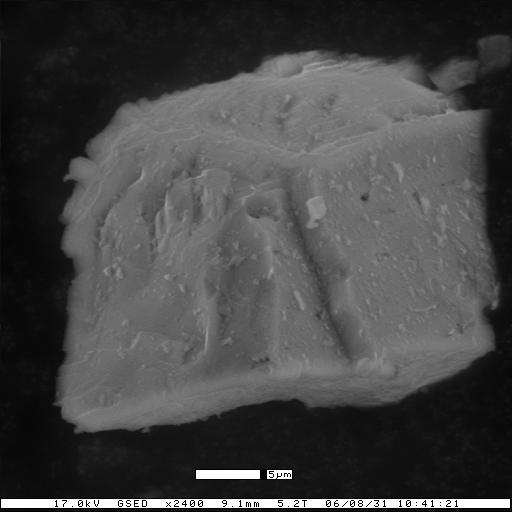
64 49 Deagglomeration Two air conveying/injection systems were tested here: high air speed venturi plus inflow injection and high air speed aspirator plus counter flow injection. Examination of collected samples from test chamber for bother cases indicated that particles bigger than 5 µm were separated from each other (Figure 4.5). Employing the high air speed venturi plus inflow injection, most large particles were found to have small particles sticking to the surfaces as shown in Figure 4.6. However, employing the high air speed aspirator and counter flow injection, no agglomeration was found at 24 km/h (Figure 4.7). At 2 and 8 km/h, only few small particles were stuck to the particles larger than 5 µm (Figure 4.8 and 4.9). Figure 4.5. ESEM image of carbon tape samples.

65 50 Figure 4.6. ESEM image of carbon tape samples collected in the test chamber at 8 km/h (Injection: high air speed venturi and inflow injection). Figure 4.7. ESEM image of carbon tape samples collected in the test chamber at 24 km/h (Injection: high air speed aspirator and counter flow injection).

66 51 Figure 4.8. ESEM image of carbon tape samples collected in the test chamber at 2 km/h (Injection: high air speed aspirator and counter flow injection). Figure 4.9. ESEM image of carbon tape samples collected in the test chamber at 8 km/h (Injection: high air speed aspirator and counter flow injection).

67 52 Conclusions In this project, a vibration hopper dust feeding system was fabricated. The repeatability and temporal variation of the discharge rate, and the deagglomeration performance were studied to evaluate the applicability of this dust feeder to wind tunnel studies. This study found that the vibration hopper dust-feeding system has the advantages of low cost, good repeatability and a wide range of dust feeding rate. It may seem to be inconvenient to get the desired feeding rate since users have to choose the correct size orifice according to Figure 4.1 and adjust the vibration pressure to obtain the dust-discharge rate to match the desired dust-feeding rate. This will not be a significant issue for studies that do not require frequent changes in the dust feed rate. Once set up for the desired experimental condition, the dust-feeding rate is repeatable for multiple experiments. For this prototype dust feeder, the temporal variation of the discharge rate was relatively constant for the time evaluated. Dust may need to be added every hour to ensure a steady feeding rate. The injection system was able to effectively prevent excessive dust agglomeration. This simple and economical vibration hopper dust feeding system appears to be acceptable for use in the dust wind tunnel for aerosol sampler studies.

68 53 MICRO VACUUM SAMPLER Introduction Previous aerosol studies focused on characterizing the sampler performance curves. Therefore, the focus has been on the initial concentration of dust in the air and the dust collected on the sampler s filter. Little attention has been given to the evaluation of the mass of dust lost in the pre-separator inlet and the corresponding PSD. This data will improve our understanding of the aspiration and transmission efficiency of the samplers. Therefore, there is a need to recover the dust loss in different parts of the PM samplers. Recovering the dust deposited on the inner walls of the samplers is challenging. Often, the dust is washed into a cup using a syringe and a brush. This washing technique is useful for inner surfaces with simple geometry. Washing is difficult for grooves and corners. Furthermore, the washing technique does not readily allow determination of the weight and PSD of the recovered dust at the same time. Vacuum sampling techniques have been widely used by industrial hygienists (Creek et al., 2006). However, the collection efficiency of the vacuum sampling technique was not well quantified before and it has never been used to collect the recovered dust on a filter. For this study, a micro-vacuum sampler was constructed. Experiments were designed to quantify the recovery ratio in order to evaluate the applicability of this technique for future aerosol studies.

69 54 Design of Micro Vacuum Sampler The primary component of the micro-vacuum sampler was a 47 mm filter holder. The inlet of the filter holder was extended by a ¼ in tube to increase the vacuuming air velocity. The tip of the tube was compressed narrower and was polished to make it easier to reach into small corners. The outlet of the filter holder was connected to a small pump. A small brush, which can reach into the inlet tube, was made to recover the dust loss to the tube and the inner wall of filter holders. Figure 4.10 shows the whole microvacuum unit, its assembly and the small brush. Figure The micro-vacuum sampler. (a) whole unit, (b) filter holder and inlet tube, (c) brush.

70 55 Methods To measure the recovery efficiency of the dust collector, fly ash was used. Fly ash was pre-weighed using plastic cups. The pre-weighed dust was then sucked into the micro-vacuum sampler and collected onto a Teflon filter. During vacuuming, some dust was lost to the inner surface of the tube and filter holder. To recover this portion of dust loss, the inner wall of the inlet was brushed with the pump on so that the dust lost to the inside wall was collected on the filter. For each experiment, the inlet tube and filter holder was brushed three times. The dust which stuck to the brush fur was also cleaned during this process. Before each experiment, the work platform was covered with plastic wraps to prevent contamination. The inner and outer surface of the vacuum sampler was cleaned with methanol. Hands were carefully cleaned before each test. Background error was caused by the entrapment of the airborne dust and by the cross-contamination from the brush and inner surface of the inlet. To estimate this background error, the inlet of the sampling unit was open to the air to sample for 2 hours and was following by brushing the inlet tube for another 1 minute. The background error was found to be negligible since only 0.2 mg dust was collected in 2 hours. For all experiments, the vacuum flow rate was ft 3 /h. All the filters were weighed with a laboratory balance (AG204, Mettler Toledo), with a precision of 0.1 mg. The whole vacuuming and brushing process took less than one minute for each sample.

71 56 Results and Discussion The collection ratio was calculated as: collection ratio = ( CollectedDust background) originaldust During all experiments, the recovery rates were above 90% (see Table 4.1), suggesting that this vacuum sampling technique may be useful in future aerosol sampling studies. Table 4.1. The experimental recovery rates (background error = 0.2 mg). Experiment Original dust (mg) Pre-weight filter (mg) Post-weight filter (mg) Collected dust (mg) Dust recovery rate (%) % % % % % % % % % % % %

72 57 IDEAL ISOKINETIC SAMPLING SYSTEM An accurate reference sampler is critical to sampler evaluation studies. Therefore, an ideal isokinetic sampling system was designed so that the velocity of the air entering the probe could be adjusted automatically to match the free-stream velocity approaching the inlet. The schematic is shown in Figure iso-kinetic nozzle pump mass flow controller V = v free air stream velocity (v) velocity transducer field controller v P RH T absolute pressure sensor relative humility & temperature sensor computer Figure Schematic of ideal isokinetic sampling system. The isokinetic sampler includes a sampler inlet, sensors, a mass flow controller and a pump (Model: M161-AT-AA1, Air Dimensions, Inc. USA). The probes used for this ideal isokinetic sampler were all conical in shape. They were machined from aluminum to fit the 47 mm sampling filter holders (see Figure 4.12).

73 58 Figure Drawing of isokinetic nozzles (unit in inches). (a) nozzle for 2 km/h, (b) nozzle for 8 km/h, (c) nozzle for 24 km/h.

74 59 The inside surface of the nozzle was polished to reduce particle loss. In this sampling system, a velocity transducer (Module 8455, TSI Inc, USA) was installed in a flexible arm so that it could be positioned upstream of the sampling inlet to monitor the wind velocity entering the sampler inlet. Another set of sensors for static pressure (Model ASCX15AN, Honeywell, Inc.), temperature and relative humility (Module HX94V, Omega Inc, USA) were installed just downstream of the working cross sectional area. The flow rate entering the probe was controlled by a mass flow controller (Module: FMA542ST-24VDC, Omega Inc, USA). The mass flow controller and all the sensors were connected to the real time field controller (Model: FP1001, FP-AI-112, FP- AO-200, National Instrument Inc. USA) which was connected to a desktop through a serial board (PCI-485, National Instrument Inc. USA ) and serial link RS232 port. All field controller units and most of the sensors were powered by 12 Vdc power supply (SFL , Solar/Heavy-duty, IL, USA). To power the pressure transducer, a low dropout positive regulator (LM1085IT-5.0-ND, was used to reduce the 12 Vdc to 5 Vdc. Except for the relative humidity and pressure transducer, all the other sensors were pre-calibrated by the manufacturers. To calibrate the relative humidity transducer, saturated lithium chloride solution and sodium chloride solution were used. The entrapped air in the containers of lithium chloride solution and sodium chloride solution provided a low RH environment of 11.3% and a high RH environment of 75.3% respectively. The probe was placed in these two environments to be calibrated following the procedure outlined in the manual. For the pressure transducer, the initial offset calibration was Vdc. To adjust the offset to exactly Vdc, the

75 60 offset adjustment circuit was used. All the circuits for the isokinetic sampling system, including the offset adjustment, are illustrated in Appendix A. The table of circuit connections is provided in Appendix B. LabView was used to develop a simple controller program (Appendix C). For every 1 ms, the program measured the real-time values of relative humility, temperature, pressure, velocity and actual mass flow rate; calculated the required mass flow rate from the accumulated averages of relative humility, temperature, pressure and velocity; compared the actual mass flow rate with the required mass flow rate; adjusted the flow rate of the mass flow controller if the difference was bigger than the systematic uncertainty. Systematic uncertainty for mass flow was calculated to be no more than 3.5% (see detailed calculation in Appendix E) using the method of Taylor Series Approximation (Kline and McClintock, 1953). The details of converting sensor signals into measured values are listed in Appendix D. The labview program also recorded the real time readings of relative humidity, temperature, pressure, wind velocity and mass flow rate to a text file. The air velocity meter (Model 8384, TSI Inc, USA) manufacturer recommends that it be returned to the manufacturer for annual recalibration. The filter screen and flow paths of mass flow controller need to be cleaned occasionally to ensure accurate performance. The temperature sensor was factory calibrated and does not require recalibration. However, the RH sensor must be recalibrated on an annual basis according to the calibration procedure outlined in the manual. The RH and temperature probes have a protective sensor filter, which needs to be cleaned to prevent clogging. Dust and

76 61 dirt may also build up on the sensor probe of the air velocity transducer (Model 8455, TSI Inc, USA). This sensor can be cleaned by dipping in a mild solvent such as alcohol and brushing with a soft bristle brush. No other maintenance is required for this type of air velocity transducer.

77 62 CHAPTER V WIND TUNNEL TESTING PROTOCOL FOR EVALUATING AEROSOL SAMPLERS USING POLY-DISPERSED PARTICLE INTRODUCTION PM 10 (which will be referred to as true PM 10 in this paper), by definition, are particles with an aerodynamic equivalent diameter (AED) less than or equal to a nominal 10 μm (USEPA, 1987). Federal Reference & Equivalent Methods PM 10 samplers are the standardized samplers that have been recommended by USEPA to measure ambient PM 10 concentration. Most FRM PM 10 samplers are filter-based, gravimetric samplers which rely on particle aerodynamics as well as air flow dynamics to separate particles. The low-volume (16.7 L/min) louvered inlet (as shown in Figure 5.1) is the most widely used inlet because of its low flow rate and satisfactory sampling characteristics at elevated wind speeds. It is incorporated in several USEPA designated reference and equivalent methods for PM 10 : Andersen Model RAAS10-100/200/300; BGI Invorporated Model PQ100/200; Grasey Andersen model SA241/SA241M; and Rupprecht and Patashnick model Partisol-FRM 2000/2025 air samplers. As shown in Figure 5.1, the louvered PM 10 dichotomous sampler inlet is composed of a louvered inlet and a PM 10 impactor. The louvered inlet is designed to aspirate sufficient PM to allow either PM 10 or PM 2.5 to be selected downstream. In the louvered inlet, the top and bottom plates are tapered 45 to minimize rain intrusion. The

78 63 presence of a deflector cone is critical since it provides a bluff body before the air is introduced into the stilling region of the inlet (Tolocka et al., 2001). The louvered PM 10 dichotomous sampler inlet was developed as a modification to the original flat-top dichotomous sampler inlet. The primary difference between the two designs are the shape of the top and bottom plates (Tolocka et al., 2001). Both inlets have been subjected to rigorous wind tunnel testing (McFarland and Ortiz, 1984; VanOsdell and Chen, 1990; Tolocka et al., 2001). Their performance was comparable. The wind tunnel testing of the louvered and flat-top PM 10 dichotomous sampler inlet shows that the cut point was within µm. Figure micron louvered PM 10 dichotomous inlet assembly (USEPA, 2001c).

79 64 Past wind tunnel studies employed the monodispersed solid/liquid aerosol as the testing PM. There are two primary concerns associated with using monodispersed particles: (1) the experimental procedure associated with mono-dispersed aerosols is tedious, time-consuming and expensive; and (2) the mono-dispersed aerosols do not fully represent real world aerosols. Therefore, a new wind tunnel testing protocol is needed to allow testing with poly-dispersed dusts. Previous studies focused on the overall sampling efficiency of the inlet and paid little attention to the aspiration and transmission efficiency of the PM 10 inlet. However, with the increasing scrutiny of sampler performance, it is necessary to quantify the aspiration and transmission efficiency. Recently, we built a dust wind tunnel that can entrain poly-dispersed solid dust. The new dust wind tunnel had an upper wind speed operational limit of 24 km/h. In the 1m 1m testing section of the wind tunnel, both the particle concentration and wind velocity was uniform within 10% of the mean, satisfying USEPA s performance requirement for wind tunnel testing of PM 10 samplers (USEPA, 1987). A vibrationhopper dust feeding system was designed to feed a wide range of solid poly-dispersed dusts (0.01 g/min 100 g/min). A micro-vacuum sampler was designed to recover >90% the dust loss to the inner walls of inlets. More details of the wind tunnel, the dust feeding system and the micro-vacuum sampler were documented elsewhere (Chen et al., 2006). Here, we describe our efforts to implement the new dust wind tunnel testing system to evaluate the performance of the louvered PM 10 dichotomous (module: PQ100/200, BGI Inc) inlet by measuring aspiration, transmission and sampling efficiency simultaneously.

80 65 EXPERIMENTAL METHODS Isokinetic Sampler A good reference sampler is critical to aerosol sampling investigation. Two types of isokinetic samplers were compared for use as a reference: a high-volume isokinetic sampler operating at 800 L/min and a low-volume isokinetic sampler operating at approximately 11 L/min. The sampling flow rate of the high-volume isokinetic sampler was adjusted manually by a valve and flow rate was determined by measuring the pressure drop across a calibrated orifice meter. For the low volume isokinetic sampler, a mass flow controller (Module: FMA542ST-24VDC, Omega Inc, USA) was used to control the sampling flow rate. A velocity transducer (Module 8455, TSI Inc, USA) was installed in a flexible arm so that it could be positioned upstream of the isokinetic sampler to monitor the wind velocity entering the isokinetic probe. Another set of sensors for static pressure (Model ASCX15AN, Honeywell, Inc.), temperature and relative humility (Module HX94V, Omega Inc, USA) were installed just downstream of the test section. The mass flow controller and all the sensors were connected to a real time field controller (National Instrument Inc. USA). A LabView program was developed to control the mass flow rate so that the velocity entering the probe was adjusted automatically to match the free-stream velocity approaching the inlet. For both isokinetic samplers, the dust loss to the inner surface was recovered to another Teflon filter using a micro-vacuum sampler. The collected dust on the inlet loss filter and sampling filter were dispensed into the same electrolyte solution for the coulter counter analysis to get a reference PSD of the dust in the air. Six experiments

81 66 were carried out for the wind speed of 8 km/h. The low-volume isokinetic sampler measured aerosol concentrations were found to be within the 10% of the high-volume isokinetic sampler. The low-volume isokinetic sampler measured particle size distribution was found to be almost the same as the high-volume isokinetic sampler. Therefore, it was concluded that the two isokinetic samplers had comparable performance characteristics. Only the low volume ideal isokinetic sampler will be used in the future as the reference sampler for the following reasons: (1) The low-volume isokinetic sampler operates at flow similar to the test samplers. (2)Using high-volume isokinetic samplers requires use of larger filters than is used for the low-volume samplers. The larger filter requires use of a different protocol for gravimetric analysis and for dispersion of particles in the Coulter Counter analysis process. Inlet Test The louvered PM 10 dichotomous inlet, used in this study, was purchased from BGI Inc (Model PQ 100/200). To measure the sampling flow rate, differential pressure transducers (PX274-05DI, Omega) were used to measure the pressure drop across the orifice meters. Prior to testing, the orifice meters were calibrated. The flow rate was manually adjusted with a valve to a nominal flow of 16.7 L/min prior to the test. Real time readings of the differential pressure transducer were recorded during the test to determine the total sampling volume. For all the experiments, the louvered PM 10 dichotomous inlet was located side by

82 67 side with the low-volume isokinetic sampler s nozzle at the center of the 1 m 1m cross-sectional testing area. Those two samplers were operated to sample the dust in the air simultaneously. Experiments were carried out for each of the three wind speed of 2, 8 24 km/h. The total blocked area of all experiment was less than 10% and the sampling time was adjusted between 30 minutes and 1 hour so that the sampling filters would collect more than 4 mg of particulate matter. Test Dust To select dust to be used as a poly-dispersed test dust, several factors were considered such as the cost, safety and physical properties of the dust. For our large wind tunnel, large amounts of dusts will be used, which limits our choices to relatively inexpensive dusts. Corn starch may be a good candidate since it is spherical in shape and has a PSD similar to many applications. However, it must be used carefully to avoid conditions were an explosion could occur. Coarse Arizona road dust was selected for this study because of four reasons: (1) it is non-explosive; (2) it is relatively cheap compared to other manufactured testing dusts such as glass beads; (3) it has a large fraction of large particles so that the dust reaching the test area will have a MMD near 10 microns; and (4) its physical properties are similar to some agricultural dusts. The test dust selected for this study was coarse Arizona road dust. Electrostatic Effect Electrostatic effect is another factor that may influence the performance of PM

83 68 samplers. During the dust feeding process, particle-to-particle and particle-to-wall contact can result in electro-statically charged particles. To minimize the electrostatic effect on sampler performance, the dust feeding system and the sampling system were electrically connected to ground. WIND TUNNEL TESTING PROTOCOL The wind tunnel testing protocol consist of: (1) pre-experimental preparation; (2) wind tunnel test; (3) dust recovery; (4) particle size analysis; and (5) post-experiment data analysis. More details can be found in Appendix H. Step 1, Pre-experiment Preparation For all experiments, 47 mm Teflon filters were used. The filter was weighed on a microbalance (Mettler M3) that has a precision of 0.01 mg after charge neutralization. Before running each test, the sampling systems for the isokinetic reference probe and the sampler inlet being tested were checked for gas leaks and the inner and outer surface of each inlet, the testing inlets and isokinetic reference probe were carefully cleaned using paper towels dampened with ethanol. The flow rate of the sampler inlet being tested was measured with an orifice meter. The orifice meter was calibrated every six months. Pressure transducers used to measure the pressure difference across the orifice plate were calibrated every six months. Before each run, the zero point of the pressure transducers was checked. Some dust deposits in the wind tunnel during each test. If this dust is re-suspended, it may introduce some error into the experiment. Therefore, before

84 69 each run, the fan was operated at its maximum speed to clean the deposited dust out of the wind tunnel. To make sure that the air will not re-entrain the deposited dust, the background dust concentration in the wind tunnel can be measured gravimetrically using a TSP sampler or in real time using a particle counter. Step 2, Wind Tunnel Test Wind tunnel testing is primarily a means to expose the sampler inlet being evaluated and the isokinetic reference sampler simultaneously to the aerosol stream in the test section of the wind tunnel. The samplers inlets were located in the same horizontal plane to reduce the error that may be caused by vertical variation of the particle size distribution, though no spatial variability was found in preliminary evaluation of the wind tunnel. For each run, several steps were performed in the following order: adjust wind speed to desired condition, activate the computer program to control sampler flow rate, begin dust feeding, begin sampling, stop the fan and dust feeding, stop sampling, stop the computer program. Step 3, Dust Recovery To get a good reference of dust concentration from the ideal isokinetic sampler, dust deposited on the inner surface of the isokinetic probe was recovered using the micro-vacuum sampling technique. The dust recovered by the micro-vacuum deposited onto a 47 mm filter. During the vacuuming process, some dust was lost to the inner surface of the nozzle of the micro-vacuum sampler. To recover this dust, a small brush was developed to reach inside the nozzle and break the dust loose while the vacuum

85 70 pump was operating. Before each test, the inner walls of samplers were cleaned thoroughly with ethanol. After each test, the probes were handled carefully to prevent the dislocation of deposited dust. Before vacuuming, the working area and the outer surface of the reference probe were wiped clean using a damp paper towel. Step 4, Particle Size Analysis The dust deposited inside the probe of the isokinetic sampler was recovered using the vacuum technique as described above. The particle size distribution of the collected aerosols were analyzed using a Coulter Multisizer 3 (Beckman Coulter, Inc. Fullerton, USA). The coulter analyses were then performed with a 100 µm aperture. The Coulter Counter Multisizer 3 was calibrated by the manufacturer annually and by laboratory technicians every 100 runs. The electrolyte solution used was composed of 5% volume of lithium chloride in methanol. Step 5, Data Analysis The diameter reported by the coulter counter was the volumetric diameter ( d e ). Aerodynamic diameter ( d ae ) is defined as the diameter of a spherical particle with a density of 1000 kg/m 3 that has the same settling velocity as the particle of interest (Hinds, 1999a). Neglecting the Cunningham slip correction factor, the aerodynamic diameter can be calculated from volumetric diameter (equation 1): d ae = d e χ ρ o 1/ 2 ρ p (5.1) For coarse Arizona road dust, the manufacturer-recommended specific gravity is 2.65.

86 71 Its shape factor (χ) is ; a value of 1.4 was used in this study. Reference concentration ( C reference ) was defined as the concentration of dust in the air. It was the sum of aerosol concentration collected with low-volume isokinetic inlet C ) and the recovered dust concentration ( C iso, vacuum ). Overall sampling efficiency ( iso E PM, sampling 10 was defined as the ratio of dust concentration in the final stage of the PM 10 sampler, to the reference concentration: E = C PM sampling samp C (5.2) 10, reference where Csamp was the aerosol concentration measured with the PM sampler. Aspiration sampling efficiency ( E aspiration penetrating the entry to the reference concentration. ) was defined as the ratio of the dust concentration ( Cinlet vacuum + Cimpactor vacuum Csamp ) Creference E aspiration =,, + (5.3) where C inlet, vacuum and impactor vacuum C, were the recovered dust loss concentration of the louvered inlet and impactor section, respectively. Transmission efficiency ( E, ) transmission n is defined as the fraction of entering particles which are transmitted down to the next stage. Assume the louvered inlet is stage 1, the impactor section is stage 2 and the sampling filter stage 3, the transmission efficiency of stage n was: 3 3 E = C C (5.4) trasmission, n, PM 10 m m= n+ 1 m= n m To obtain the cut point and slope, calculated E PM, sampling 10 was fit with a penetration efficiency curve using the Least Square Method and the SOLVER function in EXCEL.

87 72 RESULTS AND DISCUSSION Sampling Efficiency Table 5.1. Experimental plan and wind tunnel tests results of BGI PQ100/200 louvered PM 10 dichotomous inlets. Wind speed (km/h) Reference probe (mm) Dust concentration (µg/l) Replicates d 50 (µm) slope R 2 Reference MMD Reference GSD All the wind tunnel experiments that have been conducted are listed in Table 5.1. As can be seen from Table 5.1, for all three wind speeds, the cut points were within µm, satisfying USEPA s performance requirement for PM 10 samplers, either using poly-dispersed aerosols or using mono-dispersed aerosols as test dust. The standard deviation of sampling efficiency was less than 5% among three runs at 2 and 8 km/h. Both this study and previous studies (Table 5.2) found no statistical relationship between the wind speed and the cut point for this louvered PM 10 dichotomous sampler. Table 5.2. Performance of low-volume louvered PM 10 dichotomous inlets. cut point (µm) Reference # Test dust Inlet Model 2 km/h 8 km/h 24 km/h This study Coarse Arizona Road dust BGI PQ100/ McFarland and Ortiz monodispersed aerosol SA 246B VanOsdell and Chen monodispersed aerosol SA 246B VanOsdell monodispersed aerosol R&P 10 µm inlet Tolocka et al. monodispersed aerosol Dichotomous

88 73 Why does wind speed not affect the sampling efficiency of PM 10 samplers while the cut point of TSP samplers was found to be influenced strongly by the wind speeds (Wedding et al., 1977; McFarland et al., 1979; Kenny et al., 2005)? One possible explanation is that wind speed significantly affects the aspiration efficiency of sampler inlets. For TSP samplers, the aspiration efficiency will significantly affect the sampling efficiency. However, the FRM PM 10 dichotomous samplers have two stages: the preseparator and the impactor. It is not the aspiration efficiency but the transmission efficiency of the impactor that will significantly affect the sampling efficiency. Since the transmission efficiency of the impactor will not be affected by the ambient wind speed, the overall sampling efficiency will not be affected by the wind speed as long as the sampler inlet aspirates sufficient PM 10 to be selected downstream. Figure 5.2 shows examples of the sampling efficiency curves. As can be seen from Figure 5.2, the experimental penetration efficiencies of the smallest particle size were not exactly 100%. There are two possible causes for that. First, the spatial difference of aerosol concentration between the location of the isokinetic sampler and the PM 10 sampler might cause error in the sampling efficiency. For example, if the reference and the PM 10 sampler were located where the aerosol concentrations happen to be the maximum and minimum deviation from the mean: 110% and 90%, the calculated sampling efficiency could be 81.8% % of the true sampling efficiency. In future studies, the locations of reference and testing samplers can be switched in replicated experiments to account for the error caused by spatial concentration difference.

89 Figure 5.2. Wind tunnel test results for BGI PQ100/200 inlet. 74

90 75 Another possible cause was dust agglomeration. In this study, the dust in the test area was collected and examined by Environmental Scanning Electron Microscopy (Electroscan ESEM E-3). It was found that at all three wind speeds of 2, 8, 24 km/h, no agglomeration was found among particles with a volume diameter greater than 5 µm. At 2 and 8 km/h, very few small particles with volume diameter smaller than 3 µm were found stuck to particles with volume diameters larger than 5 µm. The agglomeration of small particles may affect the top most portion of the sampling efficiency curve. This small percentage of agglomeration should not significantly change the aerodynamic diameter of the larger particles and should not significantly affect the majority of the curve. As can be seen from Figure 5.1, the slope was 1.85 at 8 km/h, which is a significant deviation from the commonly assumed slope range of (Hinds, 1982). It is also observed that the highest slope coincided with the greatest deviation from 100% for small particles. Therefore, the spatial concentration difference and dust agglomeration that may cause the deviation may also cause an error in the estimated value of slope. For monodispersed aerosols, a multiplet correction method was developed to correct the error caused by multiplets in test aerosols (Ranade et al., 1990). However, for poly-dispersed aerosol, it is difficult to develop similar methods to correct the agglomeration error.

91 76 Dust Loss and Aspiration Efficiency The ratios of the dust concentration deposited at the different stages to the dust concentration measured by the isokinetic samplers are listed in Table 5.3. Also listed are the particle size distributions of the dust deposited at the different stages for the wind speed of 8 km/h. Deploying Equation , the mean aspiration, transmission and sampling efficiency of the dust were calculated and are shown in Figure 5.3. Table 5.3. The dusts deposited in different stages of the PM 10 inlet at 8 km/h. collected dust concentration MMD Stages GSD Isokinetically collected dust concentration (µm) mean Std. Dev (3 replicates) Source (isokinetic) Stage 1: Louvered inlet % 0.08 Stage 2: Impaction plate % 0.02 Stage 3: Sampling filter % 0.03 Overall aspiration efficiency 130% Due to the complex mechanisms that determine the aspiration efficiency, few publications have discussed this issue. The only identified aspiration study related to the louvered PM 10 dichotomous inlet is the study by Kenny et al. (2005). Kenny et al. tested the louvered inlet (without the impaction plate) using monodispersed solid particles. For the aerodynamic diameter of 26 microns, measured aspiration efficiencies in their study were 98% and 143% for the wind speed of 0.5 and 1 m/s, respectively. For the same aerodynamic diameter, the aspiration efficiency in this study was found to be 160% at a wind speed of 2.2 m/s (Figure 5.3). For the aerodynamic diameter of 13 microns,

92 77 measured aspiration efficiencies in their study were 110% and 127% for the wind speed of 0.5 and 1 m/s, respectively. For the same aerodynamic diameter, the aspiration efficiency in this study was found to be 134% at a wind speed of 2.2 m/s (Figure 5.3). Even though the aspiration efficiency determined in this study is higher than the one reported by Kenny et al., it was reasonable considering the higher wind speed employed in our study. The aspiration efficiency of an inlet depends on several variables such as the Stokes number, Reynolds number, and the ratio of free-stream wind velocity to the sampler inlet velocity (Kenny et al., 2005). Due to complicated nature of aspiration efficiency, more studies are needed to explain the shape of the aspiration efficiency curve. 180% 160% 140% Wind speed: 8 km/h Model: BGI PQ100/200 Dust: coarse Arizona road dust 120% efficiency 100% 80% 60% 40% 20% aspiration efficiency transmission efficiency of impactor sampling efficiency of PM10 inlet 0% aerodynamic diamter (microns) Figure 5.3. Aspiration, transmission and sampling efficiency of BGI PQ100/200 louvered PM 10 dichotomous inlet at 8 km/h (Test dust: coarse Arizona road dust).

93 78 The transmission efficiency of the impactor plate was determined as the ratio of the particles on the filter to the sum of the particles on the filter and particles deposited on the impactor. This calculation neglects the dust lost to the transition duct between the impactor and the filter holder. Therefore, the transmission efficiency curve in Figure 5.3 may not be useful for quantitative analysis. Follow-up experiments are needed to account for the dust lost to the transition duct. However, it is believed that this unaccounted-for dust-loss was negligible compared with the total dusts deposited on the filter, the louvered inlet and the impactor. Therefore, it should not affect on the values of aspiration efficiency. CONCLUSIONS This study developed a testing protocol for use of poly-dispersed dusts in order to investigate the performance of particulate matter samplers operating downwind of sources of coarse PM. The protocol primarily provides a means to expose the sampler inlet being evaluated and the isokinetic reference sampler simultaneously to a consistent aerosol stream in the test section of the wind tunnel to provide a basis to evaluate the performance of the inlet being tested. The performance of the wind tunnel facility and sampler testing protocol have been evaluated by testing a louvered dichotomous PM 10 sampler. The sampler s performance characteristics determined in this study were similar to those found in previous studies using monodispersed solid/liquid dust, indicating that our new dust

94 79 wind tunnel facility and wind tunnel testing protocol using poly-dispersed dusts is able to provide results consistent with studies with mono-dispersed dusts. This study also demonstrated the potential of using a vacuum sampling technique to recover dust deposited inside the sampler and to obtain the aspiration and transmission efficiency. The major shortcomings of this study are the lack of data on the dust lost to the transition duct between the impactor and filter holder. Even though the small amount of dust lost should not affect the aspiration efficiency curve, it may affect the accuracy of transmission efficiency calculated for a given particle size. Future study is needed to account for this dust loss. However, the preliminary results indicted that vacuum sampling techniques could be a very useful technique to obtain a detailed understanding of the performance of sampler inlets; therefore it could be very useful for future sampler design.

95 80 CHAPTER VI METHOD FOR QUANTIFYING OVER SAMPLING RATIO FOR FRM PM 10 SAMPLERS INTRODUCTION All the PM samplers have a pre-separator inlet, which allow certain dusts to penetrate. The mass penetrating the pre-separator is determined by both the PSD of the dust and the performance characteristics of the pre-separator. The sampling performance curve for the sampler inlet is commonly represented by a lognormal distribution, characterized by a cut-point (d 50 ) and a slope. The cut-point is the particle size where 50% of the PM is captured by the pre-separator and 50% of the PM penetrates to the filter. The slope is the ratio of particle sizes corresponding to collection efficiency of 84.1% and 50%. PM 10 (which will be referred to as the true PM 10 in this paper), by definition, are particles with an aerodynamic equivalent diameter (AED) less than or equal to a nominal 10 μm (USEPA, 1987). All too often, PM data obtained from PM 10 samplers are used as the accurate measurement of PM 10. Since there are no samplers that can ideally cut the PM with the particle size smaller than 10 μm AED, a common assumption made for PM 10 samplers is that the mass of particles less than 10 μm not captured by the filter is equal to the mass of particles greater than 10 μm captured on the filter. Recently, it was found that the assumption was not always correct (Buser et al., 2003; Buser, 2004): the PM 10 measured by the gravimetric PM 10 sampler tends to be higher than the true PM 10

96 81 when the MMD is greater than 10 μm, and the measured PM 10 tends to be less than the true PM 10 when the MMD is less than 10 μm. Mathematical calculations indicated the interaction of the PSD and the characteristics of PM 10 samplers resulted in an over sampling of PM 10 concentrations for most agricultural dusts. A new method was developed (Wang et al., 2005) to correct the sampling error. In this method, PM 10 and total suspended particlulate (TSP) samplers were located side by side to obtain the ratio of measured PM 10 to measured TSP. Regression equations were derived to correct the ratio of the measured PM 10 /TSP to the true PM 10 /TSP. The advantage of measuring PM 10 and TSP simultaneously is to eliminate one unknown parameter (MMD or GSD) in the calculation. However, the study assumed that the TSP measured by the TSP sampler was the true TSP, which is questionable since the cut point of TSP samplers has been reported to shift significantly with wind speed (McFarland et al., 1979; Kenny et al., 2005). The co-locating method needs to be improved by taking the error associated with TSP samplers into consideration, which is difficult mathematically. Furthermore, as recommended by Wang et al. (2005), future study should account for the variation caused by shifting of the penetration curve for PM 10 samplers in order to better simulate the performance of the PM 10 sampler in the real world. Therefore, the mathematical calculation in this study focused on the gravimetric FRM PM 10 sampler itself. The main objective of this study is to quantify, mathematically, the variation of the over sampling ratio of FRM PM 10 samplers, caused by shifting of the penetration curve, for any fixed PSD and any range of PSD parameters

97 82 (MMD and GSD). METHODS Throughout the paper, TSP true designates the true TSP in the air and PM 10,true designates the particles with AED no more than 10 μm. PM 10, measured and TSP measured do not indicate field measurements (PM 10, field and TSP field ), they are calculated from the PSD of the dusts and the penetration curve of the sampler inlet to simulate the field measurement. A standard PM 10 sampler refers to a sampler of a cut point of 10 μm and a slope of 1.5. PM 10,measured, PM 10,true and Over Sampling Ratio (E) In this study, the mass particle size distribution of the dust in the air is fitted into a one mode lognormal distribution since the aerosols dominated by sources of interested have shown monodispersed distribution. In the case that a multimodal PSD exists, this study s result from one mode distribution might still be used to predict its sampling ratio indirectly. For example, if a multimodal mass PSD is characterized by the sum of two one-mode lognormal PSDs and if the corresponding ranges of sampling ratio for each one-mode lognormal distribution can be located, the sampling ratio for multimodal PSD is the mass-percentage sum of the sampling ratios for one-mode PSD. The one mode lognormal distribution (Hinds, 1999b) is characterized by MMD and GSD (geometric standard deviation). The performance of a sampler is characterized by the penetration efficiency (P), which is characterized by the cut point (d 50 ) and slope.

98 83 PM 10, measured is measured by integrating the sampler s performance curve with the PSD of the dust. The method was introduced in detail previously (Buser, 2004; Wang et al., 2005). The appropriate equations are listed below. f ( d p / MMD, GSD) 1 exp 2π ln( GSD) ( ln d ln( MMD) ) p = 2 d p 2 ( ln( GSD) ) 2 (6.1) F ( d / MMD, GSD) ( ln d ln( MMD) ) d 1 p = exp 2 0 d p 2π ln( GSD) 2( ln( GSD) ) 2 dd p (6.2) 10, true = F (10 / MMD, GSD) TSP true (6.3) PM d = (6.4) ae d p ρ p ρ 0 P( d ae / d 50, slope) = 1 d 0 d ae 1 (ln d exp 2π ln( slope) 2 ae ln d ( ln( slope) ) ) dd p (6.5) 10, measured = TSPtrue f ( d p / MMD, GSD) P( dae / d50, PM, slope ) 10 PM dd 10 p 0 PM (6.6) where d p and d ae are the particle diameter and the aerosol aerodynamic diameter, ρ p is particle density (d p ), and ρ o is the unit density (1000 kg/m 3 ), f is the density of particles having particle diameter, F is the fraction of the particles having diameter less than d. The bias caused by the interaction of any fixed PSD and a sampler s performance characteristics is characterized by the parameter of E, which is defined as the ratio of the measured PM 10, as measured by the PM 10 sampler, to the true PM 10 : E PM 10, measured ( d50, slope, GSD, MMD) / PM 10, true = (6.7)

99 84 Simulation of Sampler Performance Characteristics To quantify the variation of the over sampling ratio (E) in real world applications, shifting of the cut point and slope for PM 10 samplers in the field needs to be known. Limited research has been carried out to study shifting of the cut point and slope in the field. The only literature identified were the wind tunnel reports on the cut points and the associated wind speeds summarized in Table 6.1. It was found that except for one case (Wedding et al., 1985), studies had not found any relationships between the wind speed and the cut point of PM 10 samplers. Table 6.1. Impact of wind speed on the cut point of PM 10 sampler (unit: µm; ρ p =1000 kg/m 3 ). Wind Speed Reference Inlet Type 2 km/h 8 km/h 24 km/h (Ranade et al., 1990) SA 321A (McFarland and Ortiz, 1984) SA 321A (Wedding et al., 1985) SA 321A (Hall et al., 1988) SA 321A (Ranade et al., 1990) Wedding (McFarland and Ortiz, 1984) Wedding (Wedding and Weigand, 1985) Wedding (McFarland and Ortiz, 1984) SA 246B (VanOsdell and Chen, 1990) SA 246B (VanOsdell, 1991) R&P 10um inlet (Tolocka et al., 2001) Dichotomous As shown in Table 6.1, all the sampler inlets (except two studies: Wedding et al and McFarland and Ortiz, 1984) satisfied USEPA standards for wind tunnel

100 85 testing(usepa, 2001c): the cut points for FRM PM 10 samplers should be within μm for 2 and 24 km/h. There are no specified tolerances for the slope of FRM PM 10 samplers in 40 CFR, part 53 (USEPA, 2001c) or any other current EPA standards. Hinds suggested that the slope of represented the slope of the lognormal collection efficiency curve associated with the PM 10 samplers (Hinds, 1982). Therefore, in this study, the range of µm and was used to characterize the shifting of the cut point and the shifting respectively for FRM PM 10 samplers in the field. Variation of Over Sampling Ratio (E) A numerical method was deployed for the calculation of E, with the continuously varying particles size d being divided into numerous discrete intervals and integration being replaced by summation. The selected interval of the particle size simulation was 0.05 microns, which was small enough to ensure simulation accuracy while maintaining computational efficiency. The simulated particles ranged from 0.1~150 microns which covered more than 99.9% of the dust fraction for most ambient PSDs. The range of MMD was from 10 to 30 µm; and the range of GSD was from 1.5 to 2.5. Those ranges are believed to encompass most agricultural dusts encountered. The cut point was simulated with an increment of 0.1µm and the slope was simulated with an increment of 0.02, resulting in 121 (11 11) simulated cut points and slopes for each pair of MMD and GSD. If the PSD of the dust in the air is constant in the field, the range of sampling

101 86 ratio can be predicted. A Matlab (Mathworks, Natich, MA) program was written to calculate the upper and lower bound on over sampling ratio for any fixed PSD. In the field, the PSD of the dust in the air is unlikely to stay constant. Instead, the PSD is more likely to vary temporally within a certain range. Therefore, there is a need to quantify the variation of over sampling ratio for different ranges of PSD parameters. The parameters of average and standard deviation are used here to characterize the variation of the over sampling ratio within any specific range of PSD parameters. A Matlab program was written to calculate the over sampling ratio for 121 pairs of MMD and GSD within the specified ranges of MMD and GSD. Each pair of MMD and GSD resulted in 121 over sampling values corresponding to different combinations of cut points and slopes. In total, any specific range of PSD parameters have 14,641 values of PM measurde /PM true, from which the mean and standard deviation were calculated. The standard deviation represents how close the sampling ratios are within the specific range of PSD. In the case that the corresponding standard deviation is significantly small, the mean may be used as correction factor (CF) to correct the error for any PSD within the specific range, CF ± = E (6.8) ( MMD ΔMMD, GSD±ΔGSD) ( d50 ±Δd50, slope±δslope, GSD±ΔGSD, MMD ± ΔMMD) RESULTS AND DISCUSSION All the results of this study were calculated for PM of a particle density of 1000 kg/m 3. For particulate matter of different particle densities, the volumetric-based MMD obtained from coulter counter needs to be converted to an aerodynamic MMD (equation

102 87 6.4) in order to use the contour maps and the tables from this study. Contour Map and Correction Factor Figure 6.1 shows the upper (E U ) and lower (E L ) bound of over sampling ratio due to the interaction of the PSD and the sampler characteristics for FRM PM 10 samplers. For any known MMD and GSD, the range of true PM 10 can be estimated: PM = PM / E, PM / E ] (6.9) 10, [ true 10, field U 10, field L Given the broiler dust, whose MMD is 24 µm and GSD is 1.6 (Redwine et al., 2002) as an example, the PM 10 measurements could be 1.6 ~ 3.6 times greater than the true PM 10 (Figure 6.1). The true PM 10 is 0.27 ~ 0.62 of the measurement values. In another words, if the measured PM 10 concentration was 200 µg/m 3, the true value was between 54 and 124 µg/m 3. In such cases, the PM 10 measurements should be corrected. Figure 6.1 also shows how sensitive the over sampling ratio is to the changes of MMD and GSD. This information may be helpful in evaluating the suitability of a PM 10 sampler for field measurements of coarse dusts. In real world application, MMD and GSD can fluctuate temporally, affected by weather conditions and human activities, etc. They are not fixed values but ranges. In situations where the variation of the over sampling ratio is small, the mean of the over sampling ratios can be used as the correction factor for PM 10 field measurement. In situations where the variation of the over sampling ratio is large, correcting the bias will be difficult for FRM PM 10 sampler. The variation of the over sampling ratio can be characterized by the standard deviation.

103 88 Figure 6.1. The upper and lower bound on over sampling ratio (E) for PM sampler with cut point of μm and slope of (ρ p =1000 kg/m 3 ). (a) upper bound of E, (b) lower bound of E.

104 89 Table 6.2 listed the mean and standard deviation of the over sampling ratios for certain ranges of PSD. For example, when MMD is from µm and GSD is , the standard deviation among the over sampling ratios is 0.082, indicating that the values of over sampling ratios are very close to each other. Therefore, the mean of 1.2 can be used to correct all the errors for all the PSD within this range. To use the correction factor for the field measurement, it must be remembered that the correction factor can only be used to adjust the measurement for limited periods, during which, the variation of PSD will not result in a large variation of the over sampling ratio. Therefore, Table 6.2 and Figure 6.1 can both provide users assistance in designing the correction scheme for their particular application. Table 6.2. The mean and standard deviation (STD) of the over sampling ratio for FRM gravimetric PM 10 samplers. (ρ p =1000 kg/m3; d 50 = μm, slope = ; 10 µm <MMD<30 µm and 1.5 <GSD< 2.5). GSD MMD mean STD mean STD mean STD mean STD mean STD μm μm μm μm μm μm μm μm μm μm

105 90 Application to PM 2.5 and TSP Sampler For TSP samplers, there is no criterion specified in the federal standards for aerodynamic cut point diameter. Aerodynamic cut point diameters of TSP samplers have been found to have a wide range (13-67 μm) (Wedding et al., 1977; McFarland et al., 1979). In this study, a cut point of μm and a slope of was used as an example for calculation. A contour map was produced for the maximum and minimum values of TSP measure /TSP true, as shown in Figure 6.2. Assuming that the cut points of TSP samplers increase from 60 to 30 μm as the wind speed increases, Figure 6.2a and Figure 6.2b represent the over/under sampling ratio at the low and high wind speeds of 8 km/h and 24 km/h respectively. The averaging approach to calculate the correction factor may not be applied to TSP samplers since their cut point was reported to decrease with increasing wind speed. If future studies confirm and quantify this relationship, a correction factor can be developed to take into account both the variation of the PSDs and the temporal variation of the wind speed. The approach to obtain the correction factor and contour maps for FRM PM 10 samplers may be applied to FRM PM 2.5 samplers. However, PM 2.5 samplers have two-stage separation for the PM and requires more careful consideration.

106 ( a ) E U 0.7 max[ TSP ] measured, d50 = 45± 15um, slope= 1.5± 0. 1 = TSP 0.65 true Geometric Standard Deviation (GSD) Geometric Standard Deviation (GSD) ( b ) E 0.55 L min[ TSP ] measured, d50 = 45± 15um, slope= 1.5± 0. 1 = TSP true Mass Medium Diameter (MMD), µm Figure 6.2. The upper and lower bound on over sampling ratio (E) for TSP sampler with cut point of μm and slope of (ρ p =1000 kg/m3): (a) upper bound of E, (b) lower bound of E.

107 92 Effect of Shifted Penetration Curve of PM 10 Sampler The above calculations incorporated two different sources of variation: the inherent bias caused by the interaction of the PSD and the fixed cut point, and the variability caused by shifting cut points and slopes of the samplers. In order to determine which is the main source of variation if a PM 10 sampler is exposed to dust of fixed MMD and GSD, two parameters of R 1 and R 2 were defined as: R 1 PM 10, measured, d 10um, slope 1.5 PM 50 = = 10, true = (6.10) R (6.11) = PM 10, measured, d = 10± 0.5um, slope= 1.5± 0.1 PM 10, measured, d = 10um, slope = R (6.12) 2, L = Min( PM 10, measured, d50 = 10± 0.5um, slope= 1.5± 0.1) PM 10, measured, d50 = 10um, slope= 1.5 R (6.13) 2, U = Max( PM 10, measured, d50 = 10± 0.5um, slope= 1.5± 0.1) PM 10, measured, d50 = 10um, slope= 1.5 R 1 shows the deviation of the measurement of a standard sampler from that of the true PM 10, eliminating the effect of varying cut points and slopes. R 2 shows how shifted cut points and slopes affect the measurement with reference to a standard PM 10 sampler. The true PM 10 can be estimated to be in the range of [ R R PM R R ] PM 2 10, field 1 2U 10, field / 1 L. Figures 6.3 and 6.4 show the contour maps for R 1 and R 2. Comparing the two figures, for the same MMD and GSD, R 1 is always greater than R 2. However, R 1 and R 2 are in the same magnitude. Simply put, the bias caused by the interaction of the PSD and the standard PM 10 sampler is always greater than the variability caused by the varied cut points and slopes within the specified tolerance, which, however, is still a significant source of variation and cannot be neglected.

108 Geometric S tandard Deviation (GSD) e PM R = , measured, d50 = 10um, slope= , true e+018 1e Mass Medium Diameter (MMD), μm 1 PM Figure 6.3. The contour maps for the ratio (R 1 ) of measured PM 10 as measured by sampler with d 50 =10 μm, slope = 1.5 to the true PM 10 (ρ p =1000 kg/m 3 ).

109 Geometric S tandard Deviation (GSD) ( a ) measured, d50 = 10± 0.5um, slope= 1.5± measured, d50 = 10um, slope= R 2, U max[ PM = PM 3 8 ] ( b ) R 2, L min[ PM = PM 0.92 measured, d50 = 10± 0.5um, slope= 1.5± measured, d50 = 10um, slope= 1.5 ] Geometric S tandard Deviation (GSD) Mass Medium Diameter (MMD), μm Figure 6.4. The contour maps for the ratio (R 2 ) of measured PM 10, as measured by sampler with shifted cut point of μm and slope of , to the measured PM 10 as measured by sampler with d 50 =10 μm, slope = 1.5 (ρ p =1000 kg/m 3 ): (a) upper bound of R 2, (b) lower bound of R 2.

110 95 CONCLUSIONS For PM of unit density, mathematical calculation for gravimetric FRM PM 10 samplers shows: If 10 µm < MMD < 30 µm and 1.5 <GSD < 2.5 (e.g. most agricultural dusts (Shaw et al., 2004)), the contour map (Figure 6.1) can be used to identify the maximum (E U ) and minimum ratio (E L ) of PM measure /PM true for fixed values of MMD and GSD. PM = PM / E, PM / E ]. 10, true [ 10, measure U 10, measure L If 10 µm < MMD < 30 µm and 1.5 <GSD < 2.5, Table 6.2 can be used to locate the mean of over sampling ratios (CF) for the different ranges of MMD and GSD. If the standard deviation is acceptable, PM, true PM10, measure / CF 10 = The inherent bias caused by the interaction of the PSD and the standard PM 10 sampler is always greater than the variability caused by the variation in cut point and slopes within the specified tolerance, which, however, is still a significant source of variation and cannot be neglected. To correct the sampling errors of the FRM PM 10 samplers, the first and most important thing is to determine the temporal, seasonal and spatial variation of the MMD and GSD of particulate matter in the field. The proposed approaches and developed figures to quantify the sampling ratio can then be used to design error-correction schema for different PM sources.

111 96 CHAPTER VII METHOD TO EVALUATE TSP SAMPLER S EFFECTIVENESS AS FIELD REFERENCE INTRODUCTION Gravimetric PM 10 samplers that behave well for urban dusts will have oversampling problems for agricultural dusts that have a mass medium diameter (MMD) greater than 10 microns, due to the interaction of particle size distribution (PSD) and sampler characteristics (Buser et al., 2003). Quantifying the relationship between PSD and this over-sampling bias is difficult in the field without a field reference of aerosol PSD and PM 10 concentration. To obtain a field reference of PM 10, gravimetric sampling is the most popular method: airborne dust can be collected on a filter using a TSP sampler and be analyzed by Coulter Counter for its PSD. In a field study conducted by the Center for Agricultural Air Quality Engineering and Science (Capareda et al., 2005), true PM 10 was calculated using measured PSD and the mass of dust collected in the sampling filter by TSP samplers. It was found that true PM 10 obtained from this approach was more accurate than that measured by the Graseby-Andersen FRM PM 10 sampler inlet (Graseby Andersen Inc, Atlanta, Georgia). To obtain a field reference of PSD, gravimetric sampling by TSP sampler followed by the Coulter Counter analysis can also be used. In the past, measured PSD of dust on the filter was used directly as true PSD of dust in the air.

112 97 There are two major concerns with using TSP samplers to obtain the field reference of PSD and PM 10 : (1) Every TSP sampler has a cut point and cannot collect all dust in the air; (2) The cut point of TSP sampler has been found to decrease with increasing wind speeds (Wedding et al., 1977; McFarland et al., 1979; Kenny et al., 2005). Therefore, the PSD of dust collected on the filter needs to be converted to the actual PSD of airborne dust. To use TSP samplers for the field reference of PM 10 and PSD, one must ensure that the shifting of the cut point of the TSP sampler will not significantly affect (1) the mass of PM 10 on the filter, and (2) the conversion of the measured PSD on the filter to the true PSD in the air. The objective of this paper is to evaluate computationally the possibility of using the TSP sampler as an accurate field reference of PSD and PM 10, taking into account the shifting of the cut point of TSP sampler. METHODS The PSD is characterized by MMD and geometric standard deviation (GSD). Throughout the remainder of this article, PSD of dust in the air and that collected by the TSP sampler are referred to as source PSD and filter PSD, respectively. Our approach to estimate the source PSD includes two steps: (1) calculate the filter PSD, given the source PSD; (2) estimate the corresponding source PSD for any filter PSD using the simulation results from Step 1 and a Least-Distance method.

113 98 Calculating Filter PSD from Source PSD Theoretically, the filter PSD can be derived by integrating the sampler s performance curve with the source PSD (Buser, 2004; Wang et al., 2005). The frequency function (f) of dust on the filter can be calculated with Equation 7.1: f filter, d d + d ( d p ) d 0 f ( d f ( d p p / MMD / MMD source source, GSD, GSD source source ) P( d ) P( d p p / d / d 50 50, slope) d( d = (7.1), slope) d( d p p ) ) where f d / MMD, GSD ) represents the frequency function of log-normally ( p source source distributed source dust(hinds, 1999b); MMD source and GSD source are the MMD and GSD of the source dust, respectively; d is the aerodynamic particle size; P( d / d50, slope) is the sampler s penetration efficiency; d 50 and slope are the cut point and slope of the characteristic curve. The f and P can be expressed by the following equations: f 1 (ln d p ln( MMD ( d p / MMDsource, GSDsource ) = exp[ 2 d 2π ln( GSD ) 2(ln( GSD )) p source source source )) 2 ] (7.2) P( d d 2 1 (ln d p ln( d50 )) / d50, slope) = 1 exp[ ] d( d 2 p ) d 2π ln( slope) 2(ln( slope)) 0 p (7.3) Using Equation 7.1, 7.2, and 7.3 to calculate filter PSD analytically, assuming a known source PSD, is impractical. The numerical method was thus deployed for this purpose, with the continuously varying particle size d being divided into numerous discrete intervals and integration being replaced by summation.

114 99 The selected interval of the particle size for simulation was 0.05 microns, which was small enough to ensure simulation accuracy while maintaining computational efficiency. The simulated particle size ranged from 0.1 to 1000 microns, which covered more than 99.99% of the dust fraction for most ambient PSDs. The range of source MMD was from 1 to 50 microns; and the range of source GSD was from 1 to 3.5 microns. Those ranges are believed to encompass the PSDs for most ambient dusts encountered. The MMD was simulated with increments of micron, while the GSD was simulated with micron increment. Each combination of MMD and GSD defined a simulated source PSD, resulting in 2,000,000 (2,000 1,000) simulated source PSDs. All the computation simulation was performed with Matlab Release 14 (The Mathworks, Inc., Natick, MA). Conventionally, GSD of filter PSD in a TSP sampler can be calculated with the following equation: MMD filter d84.1, filter GSD filter = ( + ) 2 (7.4) d MMD 15.9, filter filter where MMD filter, d 15.9,filter, and d 84.1, filter are the diameters for particles constituting 50%, 15.9%, and 84.1%, respectively, of the total mass of particles. Conventionally, these parameters are reported by Coulter Counter TM (Beckman Coulter, Inc., Fullerton, CA). Here they were determined computationally based on the simulated particle size frequency fraction ( f, ) from Equation 7.1. filter d

115 100 Estimating Filter PSD from Source PSD The results from the computer simulation was a retrieval chart which mapped source PSD (characterized by unique combinations of MMD source and GSD source ) onto filter PSD (characterized by MMD filter and GSD filter ). The following describes how this chart can be used to retrieve source PSDs based upon PSDs from TSP filters, which is characterized by MMD filter, measured and GSD filter,measured. If computer simulation had been exhaustive (i.e., all possible combinations of MMD source and GSD source had been simulated), the estimation process would be trivial. As can be seen from the previous section, MMD source and GSD source were simulated with certain step intervals and their values were not continuous. Hence resultant MMD filter and GSD filter can only take on discrete values, also. In this study, the Least-Square distance method (Equation 7.5) was used to select MMD filter and GSD filter based on known MMD filter, measured and GSD filter,measured, and subsequently retrieve MMD source and GSD source from the retrieval chart. SE = (7.5) 2 2 ( MMD filter, measured MMD filter ) + ( GSD filter, measured GSD filter ) This study attempted to retrieve source PSD for a specific range of filter PSD (MMD = microns, and GSD = 1.5-3) based on the calculated filter PSD corresponding to the source PSD (MMD = 1-50 microns, and GSD = 1 3.5). The corresponding source PSD for some filter PSD might be outside the specified range of source PSD (MMD = 1-50 microns, and GSD = 1-3.5), thus the retrieved source PSD for those filter PSD using the Least Square Method may not be correct. To exclude those

116 101 wrong retrievals, a constraint was employed: square errors between the measured and fitted filter MMD and GSD are less than and , respectively. It means that the difference between the true and fitted filter MMD and GSD is smaller than microns and 0.01 respectfully. The cut point and slope for TSP samplers are not specified in the federal standards. The cut point of TSP samplers were found to have a wide range of microns (Wedding et al., 1977; McFarland et al., 1979). In this study, the slope of TSP sampler will be assumed a constant of 1.5 for simplicity. RESULTS AND DISCUSSION Reference of PM 10 To characterize the accuracy of using the TSP followed by PM 10 fraction measurement to obtain reference PM 10, a correction factor (CF) is used. CF is defined as the ratio of the true PM 10 to the PM 10 collected by the TSP sampler. The simulated CF is calculated from Equation 6 where F is the fraction of the particles having diameter less than 10 microns. CF = F = ( MMD 10, TSP F( MMD source F ( TSP filter 10, true, GSD measured, GSD filter source TSP ) 0, d true ) 50 F( MMD f ( d, slope) p source / MMD PM = PM, GSD source, GSD 10, true 10, TSP source ) source F = F ) P( d 10, true 10, TSP p / d TSP TSP 50, true measured, slope) d( d p ) (7.6)

117 102 For a sampler of a fixed cut point, correction factors were calculated for any PSD whose MMD is within 1-50 microns and whose GSD is within For different cut points, the largest correction factor within the specified range of PSD was listed in Table 7.1. It was observed that when the cut point was greater than 30 microns, CF did not deviate significantly from 1, indicating a good estimate of true PM 10. Therefore, if the cut point of TSP sampler should be larger than 30 microns, TSP sampler could be used for the field reference of PM 10. However, shifting the cut point to 15 microns resulted in a maximum correction factor of Therefore, using maximum CF alone can not determine whether a sampler of a cut point of 15 micron can be used as a reference or not. In such case, CF charts (such as Figure 7.1) that show the correction factors of all the PSDs are needed. From Figure 7.1, it was found that the correction factors were ~1.06 when the GSD was smaller than 2.0. Therefore, even if the cut point of the TSP sampler is as small as 15 microns, the TSP sampler could still be used for the reference of PM 10 in certain cases. Table 7.1. Maximum correction factor (CF) for different cut points of TSP samplers (PM 10, true = CF PM 10, TSP, MMD source = 1-50 microns, and GSD source = ). Cut point (microns) Largest Correction Factor (CF)

118 103 Figure 7.1. Correction factors of PM 10 for a TSP sampler of a cut point of 15 microns and slope of 1.5. Reference of PSD For any sampler with a fixed cut point and slope, the source-to-filter retrieval conversion chart can be produced to illustrate the relationship between the PSD of the dust in the air and the PSD of the dust collected on the filter. Consider a TSP sampler with a cut point of 45 microns and a slope of 1.5 (Figure 7.2). The MMD and GSD of collected dust are always smaller than those of the dust to be sampled. If the true MMD and GSD in the air is 25 microns and 2, the MMD and GSD of the dust collected on the filter will be 20.5 microns and When the filter MMD is smaller than 10 microns and the filter GSD is smaller than 1.5, the filter PSD could be used directly as the PSD of the dust in the air.

119 104 Figure 7.2. Source-to-filter retrieval chart for a TSP sampler (d 50 = 45 microns; slope= 1.5): (a) filter MMD, (b) filter GSD.

120 105 Figure 7.3. Filter-to-source retrieval chart for TSP sampler (d 50 = 45 microns; slope= 1.5) (a) source MMD, (b) source GSD.

121 106 For any sampler of fixed cut point and slope, the retrieval chart for source PSD can be produced to estimate the PSD of the dust in the air given any known filter PSD. An example is shown in Figure 7.3 for a TSP sampler with a cut point of 45 microns and a slope of 1.5. The retrieval chart of source PSD may provide a simple approach for the retrieve of source PSD from the measured PSD. However, the chart was developed for a TSP sampler with fixed cut point. The isolines may shift if the cut point shifts. To address this problem, coefficient of variation is used to quantify the effect of the shifting cut point on the accuracy of using the retrieval chart for source PSD estimation. For example, Figure 7.4 is a plot of the COV of five source MMDs, which correspond to the cut points of 30, 40, 45, 50 and 60 microns. Figure 7.5 is a plot of the COV among the source MMDs corresponding to the cut point of 40, 45, 50 and 60 microns. Overall, the COV in Figure 7.5 is much smaller than the COV in Figure 7.4. It indicates that, the larger the cut point and the smaller the shifting range of the cut point, the lower the variation associated with the estimation of source MMD. Some areas in Figure 7.4 and 7.5 have values smaller than 0.1, indicating that there are only small errors associated with estimating source MMD even if the cut point shifts within the evaluated range. If the filter PSD falls into those areas, the filter-to-source retrieval chart can be employed and the TSP sampler can be accurately used for the field reference of PSD. Otherwise, care must be taken to ensure the error associated with use of PSD from the TSP sampler is acceptable.

122 107 Figure 7.4. Coefficient of variation among estimated source MMDs caused by shifted cut point (TSP samplers: d 50 =30-60 microns; slope= 1.5).

123 108 Figure 7.5. Coefficient of variation among estimated source MMDs caused by shifted cut point (TSP samplers: d 50 =40-60 microns; slope= 1.5). CONCLUSIONS In conclusion, using TSP samplers followed by Coulter Counter analysis can provide an accurate measurement of the true PM 10 in the field, since the true PM 10 is close to the PM 10 calculated from the PM 10 fraction and the mass of the dust collected by the TSP sampler. It is recommended that the cut point of TSP sampler should be larger

124 109 than 20 microns, because the shift of the cut point may affect the estimation of the true PM 10 if the cut point is smaller than 20 microns. Caution must be taken when using the PSD of the dust collected on TSP sampler s filters as a measure of the PSD of the dust in the air, because the filter MMD and GSD are always smaller than the source MMD and GSD. Only in rare cases, can filter PSD be used directly as source PSD. For a TSP sampler with a fixed cut point, the two-step approach can be used to develop the retrieval chart for source PSD (such as Figure 7.2), which provides estimated source PSD from filter PSD. However, to use the retrieval chart calculated from a fixed cut point, it is recommended that the effect of cut point shifting on the accuracy of the conversion method should be assessed. For the same filter PSD, the variation of the corresponding source PSD for different cut points, can be characterized by COV. If the corresponding COV is greater than the acceptable error associated with a potential study, TSP sampler should not be used as the reference for field study. In summary, the findings of this study provides a method to evaluate the use of TSP samplers for field evaluation of aerosol samplers in future studies.

125 110 CHAPTER VIII CONCLUSION AND FUTURE WORK CONCLUSIONS This dissertation developed the methodology to correct the sampling error associated with the FRM PM 10 sampler: wind tunnel testing facilities and protocol, computational qualification of the variation of the over-sampling ratios of FRM PM 10 samplers, and computational evaluation of TSP sampler effectiveness as a potential field reference. In order to evaluate PM samplers experimentally, this study designed a full-scale dust wind tunnel through small-scale testing. Small-scale testing is a good way to gain experience and to predict qualitatively the performance of the full-scale wind tunnel. The small-scale wind tunnel testing indicated that the Generic Tee Plenum System (GTPS) was an adequate mixer. Based on the small-scale testing, a full-scale wind tunnel that satisfies USEPA s wind tunnel requirements for testing PM 10 samplers has been constructed. Three systems were developed for this wind tunnel testing of aerosol samplers. A low cost dust feeding system was designed, which is able to de-agglomerate and disperse dust into the wind tunnel over a wide range of concentrations (0.1 g/min 100 g/min). A micro-vacuum sampler was designed to recover >90% of the dust loss to the inside of sampler inlets. An ideal isokinetic sampling system was designed so that the velocity of the air entering the probe will be adjusted automatically to match the free-stream

126 111 velocity approaching the inlet. The ideal isokinetic sampling system was used as the reference for all wind tunnel testing. Previous wind tunnel studies employed mono-dispersed particles. To better simulate the performance of PM samplers in the real world, non-spherical poly-dispersed particles were utilized. To evaluate the wind tunnel facilities and new wind tunnel testing protocol using poly-dispersed particles, this study tested the louvered PM 10 dichotomous inlet, the most widely tested inlet. The results of the dust wind tunnel testing indicated that the cut point of louvered dichotomous PM 10 inlet was within USEPA s requirement and the wind speed did not affect the cut point of the inlet. These results were comparable to previous wind tunnel tests, indicating that our new dust wind tunnel facility and wind tunnel testing protocol using poly-dispersed dusts was able to provide results consistent with previous studies. This study used the range of over-sampling ratio to quantify the variation of sampling errors caused by shifting cut points and slopes. This study also proposed the averaged over-sampling ratios and its deviation to characterize the variation of sampling errors within certain ranges of PSDs. Correction charts and tables were developed to assist in understanding the over-sampling problem in field applications. All the computations were based on the assumption that the cut point and slope of the PM 10 sampler shift independently with the wind speed within the specified tolerance of µm and , respectively. To evaluate the validity of the correction charts and tables, the sampler s performance characteristics must be evaluated in a controlled experimental environment and in the field.

127 112 In order to evaluate the performance characteristics of PM samplers in the field, an accurate reference is needed. This study evaluated computationally the TSP sampler s effectiveness as a field reference. The estimated PM 10 concentration obtained by PSD analysis of TSP sampler filter was calculated to be comparable to the true PM 10 when the TSP sampler s cut point is greater than 20 microns. Hence, the use of the TSP sampler for the field reference of PM 10 concentration can be recommended. The applicability of the TSP sampler as the field reference of aerosol PSD needs to be determined on a caseby-case basis. First, the range of the TSP cut point and the range of filter PSDs must be known. The effect of varying cut points on estimation of true PSD can then be estimated. If the varying cut point will not significantly affect the estimation of true PSD, the aerosol PSD measured by TSP sampler can be converted to the true aerosol PSD. Following the method outlined in Chapter VII, the chart for the Coefficient of Variation (COV) among the estimated true PSD can be produced which can help determine the TSP sampler s effectiveness as a field reference. A retrieval chart was generated to convert PSD from a TSP sampler (with a fixed cut point) to true PSD via a Least- Distance means. Overall, the TSP sampler could be used as the field reference of PM 10 concentration. However, obtaining PM 10 sampler s sampling characteristics (cut point and slope) in the field will depend on a good field reference of aerosol PSD. This depends on many factors that affect the conversion of measured PSD by TSP sampler to the true aerosols PSD: the variation of the wind speed, the variation of the cut point with the wind speed and the range of aerosol PSDs.

128 113 FUTURE WORK For the field study of sampling characteristics, a good reference of aerosol PSD is needed. In order to have a good field reference of PSD, future studies should focus on designing a TSP sampler whose cut point is as large as possible and the shift of cut point with the wind speed is as small as possible so that it will not affect significantly the conversion of the filter PSD to source PSD. The isokinetic nozzles used in this study were found to be associated with 10%~20% dust loss to the inner surface, which were similar to past studies (Fan et al., 1992). Current isokinetic nozzles require the recovery of lost dust. In order to save the challenges associated with dust recovery, shrouded probe (Chandra and McFarland, 1997), a new design of isokinetic nozzle may be deployed in the future to reduce the dust loss. The current wind tunnel facilities were designed in a way to minimize the manufacturing and operational cost. Much can be done to improve the current wind tunnel facilities and testing protocol. The current dust feeding system uses aerodynamic forces to break up most agglomerations. However, if the electrostatic charges carried by the aerosols can be neutralized, the dust could be further de-agglomerated. In addition, the dust lost inside the wind tunnel is very significant since we have a big wind tunnel. Reducing the deposited dust and maintaining the uniform dust concentration profile remain a great challenge for future studies.

129 114 REFERENCES Anand, M., A. R. McFarland, and K. R. Rajagopal Gas mixing for achieving suitable conditions for single point aerosol sampling in a straight tube: experimental and numerical results. Health Phys 84: Belyaev, S. P. and L. M. Levin Techniques for collection of representative aerosol samples. J Aerosol Sci 5: Buser, M. D Errors associated with particulate matter measurements on rural sources: appropriate basis for regulating cotton gins. Ph.D. College Station: Texas A&M University, Biological and Agricultural Engineering Department. Buser, M. D., C. B. Parnell, B. W. Shaw, and R. E. Lacey Particulate matter sampler errors due to the interaction of particle size and sampler performance characteristics: PM 10 and PM 2.5 ambient air samples. In 2003 ASAE Air Quality Meeting Raleigh, North Carolina. Capareda, S. C., C. B. Parnell, B. W. Shaw, and J. D. Wanjura Particle size distribition analyses of agricultural dusts and report of true PM 10 concentration. In 2005 ASAE Annual International Meeting. Tampa, Florida. ASABE. Chandra, S. and A. R. McFarland Shrouded probe performance: variable flow operation and effect of free stream turbulence. Aerosol Sci Technol 26: Chen, J., B. W. Shaw, C.A.Ortiz, W. B. Faulkner, and C.Parnell A new dust wind tunnel for particulate matter sampling study. In 2006 ASABE Annual International Meeting. Portland, Oregon. Creek, K. L., G. Whitney, and K. Ashley Vacuum sampling techniques for industrial hygienists, with emphasis on beryllium dust sampling. J Environ Monit 8: Crewdson, B. J., A. L. Ormond, and R. M. Nedderman Air-impeded discharge of fine particles from a hopper. Powder Technol 16: Fan, B., A. R. McFarland, and N. K. Anand Aerosol-particle losses in isokinetic sampling probe inlets. Environ Sci Technol 26: Federal-Register Revisions to the national ambient air quality standards for particulate matter Register F. Friket, M. B The cause of the symptoms found in the Meuse Valley during the fog of December Acad R Med Belg 2:

130 115 Hall, D. J. and M. A. Emmott Some comments on the effects of atmosphericturbulence on ambient particle samplers. J Aerosol Sci 25: Hall, D. J., S. L. Upton, and G. W. Marsland Designs for a deposition gauge and a flux gauge for monitoring ambient dust. Atmos Environ 28: Hall, D. J., S. L. Upton, G. W. Marsland, and R. A. Waters Wind tunnel measurements of the collection efficiency of two PM 10 samplers: the Sierra- Andersen Model 321A hi-volume sampler and the EPA prototype dichotomous sampler. LR669. Stevenage, U.K, Warren Spring Laboratory. Han, T Evaluation of mixing in three duct configurations and development of a Generic Tee Plenum System (GTPS) for application to single point aerosol sampling. MS thesis. College Station: Texas A&M University, Department of Mechanical Engineering. Han, T., D. O'Neal, A. R. McFarland, J. Haglund, and C. A. Ortiz Evaluation of mixing elements in an L-shaped configuration for application to single point aerosol sampling in ducts. HVAC&R Research Journal 11: Han, T., D. O'Neal, and C. A. Ortiz Generic-tee-plenum mixing system for application to single point aerosol sampling in stacks and ducts. Health Phys 92: Heist, D. K., J. Richarmond-Bryant, A. Eisner, and T. Conner Development of a versatile aerosol generation system for use in a large wind tunnel. Aerosol Sci Technol 37: Hinds, W. C. 1982, Chapter V, Straight line acceleration and curvilinear particle motions. In Aerosol Technology: Properties, Behavior, and Measurement of Airborne Particles. Hinds WC, ed. New York, John Wiley & Sons, Inc. Hinds, W. C. 1999a, Chapter III, Uniform particle motion. In Aerosol Technology: Properties, Behavior, and Measurement of Airborne Particles (2 ed.), Hinds WC, ed. New York, John Wiley & Sons, Inc. Hinds, W. C. 1999b, Chapter IV, Particle size statistics In Aerosol Technology: Properties, Behavior, and Measurement of Airborne Particles (2 ed.), Hinds WC, ed. New York, John Wiley & Sons, Inc. Hunt, M. L., R. C. Weathers, A. T. Lee, C. E. Brennen, and C. R. Wassgren Effects of horizontal vibration on hopper flows of granular materials. Phys Fluids 11:

131 116 Kenny, L., G. C. Beaumont, A. Gudmundsson, A. Thorpe, and W. Koch Aspiration and sampling efficiencies of the TSP and louvered particulate matter inlets. J Environ Monit 7: Kline, S. J. and F. A. McClintock Describing uncertainties in single-sample experiments. Mechanical Engineering 75: 3-8. Kollmann, T. and J. Tomas Effect of applied vibration on silo hopper design. Part Sci Technol 20: Kratz, S., J. Rogasik, and E. Schnug Environmental impacts of broiler production: a literature review. Landbauforsch Volk 50: Kurkela, J. A., D. P. Brown, J. Raula, and E. I. Kauppinen New apparatus for studying powder deagglomeration. Powder Technol 177: Lai, C. Y. and C. C. Chen Performance characteristics of PM 10 samplers under calm air conditions. Journal of the Air & Waste Management Association 50: Lange, J., J. C. Parnell, S. Capareda, R. Lacey, B.Sahw, and S. Mukhtar Engineering analysis of particulate matter emissions from the Buckeye Marseilles laying hen facility. College Station, CAAQES, Department of Biological and Agricultural Enginerring, Texas A&M University. Logan, W. P. D Mortality in the London fog incident. Lancet 1: McFarland, A. R. and C. A. Ortiz Characterization of Sierra-Andersen PM-10 inlet model 246B. Texas A&M University. College Station, TX, Air quality Laboratory Report. McFarland, A. R., C. A. Ortiz, and R. W. Bertch A 10 mu-m cutpoint size selective inlet for hi-vol samplers. JAPCA J Air Waste Ma 34: McFarland, A. R., C. A. Ortiz, and C. E. Rodes Characteristics of aerosol samplers used in ambient air monitoring. In 86th National Meeting of the American Institute of Chemical Engineers. Houston, TX. Milliman, E. M., D. P. Y. Chang, and O. R. Moss A dual flexible-brush dust-feed mechanism. American Industrial Hygiene Association Journal 42: Nedderman, R. M., U. Tuzun, S. B. Savage, and G. T. Houlsby The flow of granular-materials.1. discharge rates from hoppers. Chem Eng Sci 37:

132 117 NRC Air emissions from animal feeding operations: current knowledge, future needs. Washington, DC: National Academy Press Omland, O Exposure and respiratory health in farming in temperate zones - a review of the literature. Ann Agr Env Med 9: Paik, S. Y. and J. H. Vincent Aspiration efficiencies of disc-shaped blunt nozzles facing the wind, for coarse particles and high velocity ratios. J Aerosol Sci 33: Paik, S. Y. and J. H. Vincent The orientation-averaged aspiration efficiency of IOM-like personal aerosol samplers mounted on bluff bodies. Annals Of Occupational Hygiene 48: Parnell, C. B., D. D. Johns, R. D. Rutherford, and K. J. Goforth Physical properties of five grain types. Environ Health Perspect 66: Ranade, M. B., M. C. Woods, F. L. Chen, L. J. Purdue, and K. A. Rehme Windtunnel evaluation of PM 10 samplers. Aerosol Sci Technol 13: Redwine, J. S., R. E. Lacey, S. Mukhtar, and J. B. Carey Concentration and emissions of ammonia and particulate matter in tunnel-ventilated broiler houses under summer conditions in Texas. Transactions of the Asae 45: Reist, P. C. and L. Taylor Development and operation of an improved turntable dust feeder. Powder Technol 107: Rodes, C. E., D. M. Holland, L. J. Purdue, and K. A. Rehme A field comparison of PM 10 inlets at four locations. J Air Pollut Control Assoc 35: Rylander, R Organic dusts - from knowledge to prevention. Scand J Work Environ Health 20: Shaw, B. W., R. E. Lacey, S. Capareda, C. B. Parnell Jr, J. Wanjura, L. Wang, and F. W.B. Application of the national ambiant air quality standards (NAAQS) in urban versus rural environments. In ASAE/CSAE Annual Internationsl Meeting, Ottawa, Ontario, Canada, Sweeten, J. M., J. R. Clark, W. L. Harman, B. L. Harris, B. H. Johnsen, W. R. Jordan, M. J. McFarland, C. B. Parnell, S. C. Ricke, and R. B. Schart Concentration animal feeding operations in Texas: an extension, research and educational action plan for environmental quality management.. Executive Committee, The Agricultural Program, Texas A&M Univesity, College Station, Texas.

133 118 Tolocka, M. P., T. M. Peters, R. W. Vanderpool, F. L. Chen, and R. W. Wiener On the modification of the low flow-rate PM10 dichotomous sampler inlet. Aerosol Sci and Technol 34: USDA-AAQTF Air quality research and technology transfer white paper and recommendations for concentrated animal feeding operations. Washington D. C. United States Division of Agriculture: Agricultural Air Quality Task Force. USEPA Ambient air monitoring reference and equivalent methods: Federal Register 40 CFR Part : July 1. College Park, Maryland, Office of Federal Register. USEPA Chapter IV: sampling and analysis methods for particulate matter and acid deposition. In Air Quality Criteria for Particulate Matter. May 7. Research Triangle Park, North Carolina, National Center for Environmental Assessment. USEPA. USEPA. 2001a. Ambient air monitoring reference and equivalent methods. Federal Register 40 CFR, part 53. College Park, Maryland, Office of Federal Register. USEPA. 2001b. List of designed reference and equivalent method. National Exposure Research Laboratory. Available at Accessed January 18, USEPA. 2001c. National primary and secondary ambient air quality standards. Federal Register 40 CFR Part 50. College Park, Maryland, Office of Federal Register. USEPA. 2001d. Reference method for the determination of particulate matter as PM 10 in the atmosphere. Federal Register 40 CFR, Part 50, Appendix J. College Park, Maryland, Office of Federal Register. Vanderpool, R. W., T. M. Peters, S. Natarajan, D. B. Gemmill, and R. W. Wiener. 2001a. Evaluation of the loading characteristics of the EPA WINSPM2.5 separator. Aerosol Sci and Technol 34: Vanderpool, R. W., T. M. Peters, S. Natarajan, M. P. Tolocka, D. B. Gemmill, and R. W. Wiener. 2001b. Sensitivity analysis of the USEPA WINSPM2.5 separator. Aerosol Sci and Technol 34: VanOsdell, D. W Wind tunnel test report No. 29A: test of the Ruppecht and Patashnick TEOM PM 10 sampler inlet at 2 and 24 km/h. EPA Contract No Research Triangle Park, North Carolina. Research Triangle Institute

134 119 VanOsdell, D. W. and F. L. Chen Wind tunnel test report No. 28: test of the Sierra Andersen 246B dichotmous sampler inlet. EPA Research Triangle Park, North Carolina. Research Triangle Institute. Wagner, J. and D. Leith Passive aerosol sampler. Part I: Principle of operation. Aerosol Sci Technol 34: Wang, L., C. B. Parnell, B. W. Shaw, R. E. Lacey, M. D. Buser, L. B. Goodrich, and S. C. Capareda Correcting PM 10 over-sampling problems for agricultural particulate matter emissions: preliminary study. Transactions of the ASAE 48: Wanjura, J. D Engineering approaches to address errors in measured and predicted particulate matter concentration. College Station: Texas A&M University, Biological and Agricultural Engineering. Wedding, J. B., A. R. McFarland, and J. E. Cermak Large particle collection characteristics of ambient aerosol samplers. Environ Sci Technol 11: Wedding, J. B. and M. A. Weigand The Wedding ambient aerosol sampling inlet (D 50 =10-Mu-M) for the high-volume sampler. Atmos Environ 19: Wedding, J. B., M. A. Weigand, and Y. J. Kim Evaluation of the Sierra-Andersen 10-mu-m inlet for the high-volume sampler. Atmos Environ 19: Wiener, R. W., K. Okazaki, and K. Willeke Influence of turbulence on aerosol sampling efficiency. Atmos Environ 22: Witschger, O., R. Wrobel, J. F. Fabries, P. Gorner, and A. Renoux A new experimental wind tunnel facility for aerosol sampling investigations. J Aerosol Sci 28: Zamel, J. M. and M. Petach Gas grain simulation experiment, module conceptual design and gas grain simulation facility, breadboard development. NASA Contractor Report No Moffett Field, California.

135 APPENDIX A CIRCUIT OF IDEAL ISOKINETIC SAMPLING SYSTEM LN G +- FieldPoint (FP-1001) Voltage Input (AI-112) Current output (AO-210) address: 0; band: 300 v v v v 12 VDC 6A - + RXD+ RXD- GND TXD- TXD+ v c v c c c c v 5V voltage regulator 200 Ohm RX- RX+ Ground TX- TX DB-9 connector cable ground VDC (-) (+) offset adjustment (+) + output ground T output RH output V -V Velocity Transducer Pressure Transducer Temperature & Pressure Transducer 121

136 APPENDIX B CIRCUIT CONNECTION TABLE FOR IDEAL ISOKINETIC SAMPLING SYSTEM sensors Pins cable Connector pins Pins Field Points Velocity Transducer Pressure Sensor Temperature & RH transducer Mass Flow Controler 485 signal + V red pin VDC -V green pin 5 ground - signal black pin 8 pin 18 + signal white pin 7 pin 2 AI-112 pin 4 (ground) white with black stripe pin VDC pin 2 (Vs) red with black stripe pin 18 - VDC pin 3 (output) blue pin 20 pin 11 AI-112 pin 1 (external offset adjustment) orange pin 19 pin 1 (power supply) red pin VDC pin 2 (ground) green pin 5 - VDC pin 3 (temperature output) black pin 8 pin 16 pin 4 (RH output) white pin 7 pin 15 AI-112 pin 1 (AI com) black pin 24 pin 2 (AI Vin) orange pin 7 AI-112 pin 3 (GND PS) green ground pin 5 (GND PS) green ground pin 7 (12V PS) red +12 VDC pin 8 (AO IO) white pin 1 AO-210 pin 10 (AO COM) blue pin 2 AO-210 pin 13 (12V PS) red + 12 VDC pin 15 (chasis ground) red with black stripe chasis ground pin 4 (RX +) orange RXD+ pin 5 (RX - ) white RXDpin 1 (GND) green Ground FP-1001 pin 9 (TX - ) black TXDpin 8 (TX +) red TXD+ 122

137 APPENDIX C LABVIEW CODE FOR IDEAL ISOKINETIC SAMPLER Note: The logic description of the code can be found in page

138 124 APPENDIX D CONVERSION OF INSTRUMENT SIGNALS TO MEASURED VALUES FOR IDEAL ISOKINETIC SAMPLING SYSTEM Parameters Analogue to Digital Conversion Relative Humidity RH = V (voltage) Temperature o T ( C) = 100 V ( voltage) o T ( K) = T ( C) Pressure Wind velocity Mass flow controller Reading Writing 10 V ( voltage) P( psia) = 2.5 / 3 3 P( Pa) = ( V ( voltage) 0.25) E E out 0 v = EFS E0 where vfs* = fullscale veloctiy setting ( m / s) v = measured velocity( m / s) Eout = measured output( voltage) E0* = zero flow output( voltage) EFS* = Fullscale output( voltage) Note, v FS, E, E is set up in the control panel of the velocity 0 FS transducer following the instructions in page 8 of the Operation and Service Manual of Model 8455/8465/8475 Air Velocity Transducer. Currently, E 0, and E FS is set to be 1 and 5 voltage Where M actural ( kg / s) = V ( voltage) 2 I ( amp) = 48 A( m ) v( m / s) v FS 2 A = nozzle opening area ( m ) v = measured velocity( m / s)

139 125 APPENDIX E SYSTEMATIC UNCERTAINTY OF MASS FLOW CONTROL USED IN IDEAL ISOKINETIC SAMPLING SYSTEM Let Y be a function of independent variables x 1, x 2 x n and let β, β 1, β 2 β n are the systematic uncertainty of Y, x 1, x 2 x n correspondingly. Then the systematic uncertainty for Y can be calculated by: β = Y β + Y β Y β ) 2 2 ( 1) ( 2 )... ( n x1 x2 x n To ensure the ideal Isokinetic sampling of the dust, the parameter that we are concerned with is: ΔM = M M = M = M actual actual actual = F( M ρ v A Pa RH Ps RH P, s ( + ) v A T T, P, P, T, RH, v, A) actual required a where: M actual = actual mass flow rate of mass flow controller M required = the required mass flow rate to ensure the Isokinetic sampling ρ = density (kg/m 3 ) v = wind speed (m/s) A = nozzle opening area (m 2 ) RH = relative humidity P s = saturated pressure of water (Pascals) P a = absolute pressure (Pascals) T = temperature (degk = deg C ) s Table E.1. Instrument accuracy specifications. Parameter Instrument Accuracy V +2.0% reading + 0.5% of full scale Module 8455, TSI Inc, USA of selected range T Module HX94V, Omega Inc, USA +0.6 C P a Model ASCX15AN, Honeywell, Inc +0.5% of full scale P s Steam Tables Pisa RH Module HX94V, Omega Inc, USA + 2.0% Mass Flow Model FMA542ST-24VDC, Omega Inc, +1.5% of full scale Nozzle opening Diameter = 0.78/0.4/ Three size has been manufactured area (A) inch;

140 126 Table E.2. The systematic uncertainties for different variables. Wind speed β v β A β (m/s) (m 2 M actual β β T P β a P β s RH ) (kg/s) (K) (Pascal) (Pascal) 2 km/h E-07 8 km/h E E km/h E-07 To facilitate the calculation of the uncertainty for Δ M, the following conditions are used: T=298 K, RH=0.95, Ps=4246 Pisa, and Pa= Pisa. The accuracy of the independent variables are listed in Table E.1. From Table E.1, the systematic uncertainty for each variable for different wind speed are calculated and listed in Table E.2. The systematic uncertainty for β ΔM = ΔM ( M ΔM + ( β RH Δ M is: ) 2 ) 2 ΔM + ( v β ) ΔM + ( β P ) a P 2 2 ΔM + ( A β ) ΔM + ( β P ) s P where ΔM = 1, M actual ΔM Pa RH Ps RH Ps = ( + ) A, v T T ΔM Pa RH Ps RH Ps = ( + ) v, A T T ΔM Pa RH Ps RH Ps va = ( + ), 2 T T ΔM Ps 1 1 = ( ) va, RH T ΔM va =, Pa T ΔM RH 1 1 = ( ) va, P T s actual β M actual RH a v s A 2 2 ΔM + ( T β ) T 2

141 127 APPENDIX F WIND TUNNEL TESTING PROTOCOL FOR PM SAMPLERS PREPARATION Weigh Filter Step 1, Step 2, Step 3, Step 4, Label the 47-mm and 8 x10 Teflon filters numerically using permanent marker; store each 47-mm filter in a Petri dish and each 8 x10 filter in an electrostatic bag/aluminum sheet before usage. Using a scalar that has a precision of 0.01 mg. Clean the inner surface using the computer vacuum before usage Put one scale ionizer tray A at the center of the scalar. Zero the weight. Before weighing, put the filter on another scale ionizer tray B outside of the scale. Then weigh the filter on ionizer tray A inside of the scale. Repeat the weighing for 3 times and record all the readings. The average of the readings is the weight of the filter Pre-weigh seventeen 47-mm Teflon filters, one 8 x10 filter and three glass fiber filters for each run. Store 47-mm Teflon filters in Petri dishes and store the 8 x10 filter in a piece of aluminum foil Check Gas Leak of Low-Volume Ideal Isokinetic Sampler The low volume ideal Isokinetic sampler is controlled by the mass flow controller. The leaking can be checked by the read out from the mass flow controller. Step 1, Step 2, Step 3, Step 4, Step 5, Step 6, Load a Teflon filter on the Isokinetic sampler s inlet. Connect the corresponding hose to the quick connector which connects to mass flow controller. Turn on the power for ideal Isokinetic controlling system. Open the Labview program MFC leaking check under the folder of C:\Ideal Isokinetic sampler. Turn on the pump and block the sampling inlet with a rubber stopper Click on the run button. If the readings are lower than 0.2, there is almost no leaking. If the readings are larger than 0.2, reload the filter, check the O-ring between the sampler holder and the nozzle. Fix the leaking problem. (The majority of the leaking comes from the sampler inlet. However, it is difficult to limit that portion of leaking.) Repeat step 1 - step 5. Click the stop button to stop the program, turn off the power for ideal Isokinetic controlling system. Unload the filters

142 128 Check gas leak of PM10/TSP Sampling System The high volume Isokinetic sampler, the low-volume sampling unit for PM 10 and TSP inlet has an orifice and a pressure transducer to measure the pressure drop across the orifice. The leaking can be checked by the read out from the pressure transducer. It is difficult to block the sampler inlet of PM10/TSP samplers. Therefore, only the leaking from the part before the inlet was checked. Step 1, Step 2, Step 3, Step 4, Step 5, Connect the pressure transducer to the field controller according to Appendix A. Turn on the pump and block the inlet of tubing Turn on the power for sampling system. Open the Labview program Low volume leaking check under the folder of C:\Ideal Isokinetic sampler. Click on the run button. If the absolute value of the readings are smaller than 0.02, there is almost no leaking. If the absolute value of the readings are larger than 0.02, fix the leaking problem. Repeat step 1-5 Click the stop button to stop the program, turn off the power for ideal Isokinetic controlling system Low Volume Isokinetic Sampling System The low volume isokinetic sampling system has a gas flow meter (RMB- 35, IN, Dwyer Instruments Inc) to measure the volume flow rate and a magnehelic differential pressure gauge (Model 2100, IN, Dwyer Instruments Inc) to measure the pressure drop. Step 1, Step 2, Turn on the pump and block the inlet of tubing If the volume flow rate drop to zero, there is no leaking. Otherwise, fix the leaking problem. Calibrate High Volume Isokinetic Sampler Step 1, Connect the hose to a high volume Digital air flow calibrator. Step 2, Zero the magnehelic pressure gage Step 3, Turn on the pump, adjust the valve to achieve different pressure drop across the orifice. Record the volume flow readings and the corresponding pressure drop across the orifice shown on the magnehelic pressure gage. Calibrate Orifice Plate (See details in Appendix G) Calibrate Pressure Transducer (See details in Appendix H)

143 129 WIND TUNNEL TESTING Step 1, Step 2, Pre-clean the dust wind tunnel Turn on the exhaust fan and the blowing fan. Let the fan run at its maximum speed for 5 minutes so that the dust deposited inside the wind tunnel will be cleaned before each experiment. Dust Feeder Position the agitation rod so that the tip of the rod is right above the exit hole of the hopper. Rotate the rod to make sure that it does not hit the inner wall of dust feeder. Fill the dust feeder with the desired feeding material. Turn on the vibrator and the rod; adjust the vibration pressure and the rotation rate of the agitation rod to desired values. Let the dust feeder run for a while to make sure that it is feeding continuously. Turn off the dust feeder. Step 3, Step 4, Step 5, Clean Samplers Pre-clean the samplers using the small desktop vacuum. Wet the towel paper using isopethenol and wipe the inner surface of the samplers clean. Assemble the samplers together. Turn on controlling system & check the function of pressure transducer The controlling system need 15 minutes to warm up before being put into use. Open the Labview program low volume leak check under the folder of C:\Ideal Isokinetic sampler. Click on the run button. The interface of Labview Program will show the required pressure drops and the actual pressure drops for each sampling unit. Turn on the transformer of pressure transducers. Check the actual pressure drop on the computer screen. If the read out value (absolute) is smaller than 0.02, the pressure transducer is zeroed. Otherwise, zero it according to Appendix H. Pre-adjusting sampling flow rate PM 10 /TSP/High volume Isokinetic sampler Turn on the pump. Manually adjust the valves so that the actual pressure drop is close to the required pressure drop. Turn off pump Low volume Isokinetic sampler Turn on the pump, and manually adjust the valve so that the sampling flow rate reaches the desired flow rate. Turn off pump. High volume Isokinetic sampler Turn the power on, and adjust the valve manually so that the pressure drop across the orifice reaches the desired value. Turn off power

144 130 Ideal volume Isokinetic sampler No need to pre-adjust the ideal Isokinetic sampler. Step 6, Load filters Carefully load the pre-weighed filters into the filter holders using a nipper. Record the sampling filters number for different sampler s inlets. The test cross section is divided into 9 grids. Record the corresponding location of different sampler inlets Step 7, Step 8, Check the setup of the velocity transducer panel Follow the instruction posted above the velocity transducer panel. Adjusting wind speed Turn on the exhaust fan and driving fan. Allow enough time for the fan to accelerate to its desired speed. Then open the Labview program Ideal Isokinetic sampling under the folder of C:\Ideal Isokinetic sampler. In the user-interface, select the diameter of nozzle opening and the range of velocity. Click on the run button. The computer screen will show the real-time wind speed. Adjust the frequency of driving fan so that the averaged wind speed on the computer s screen is close to the desired wind speed (2 km/h, 8 km/h or 24 km/h). All The data will be automatically saved in the file of textfile.txt under the folder of C:\Ideal Isokinetic sampler. Step 9, Step 10, Step 11, Start Turn on the dust feeder. If low volume isokinetic sampler is used, record the initial volume flow rate and pressure drop for the low volume Isokinetic sampler. Turn on the pumps for samplers. End Turn off the dust feeder. Let the exhaust fan and the driving fan blow for another 5 minutes. Turn off the pumps for samplers. Stop the driving fan by pressing the button of stop in the VFD. If low volume isokinetic sampler is used, record the volume flow rate and pressure drop before turn off pump. Stop the Labview program and turn off the power for the sensor system. Sampling filters For each sampler; wipe the dust on off the outer surface of PM inlets using wet towel paper. Unscrew the nozzle from the filter holder, and carefully remove the filter from the filter holder to an

145 131 aluminum foil using a nipper. Put all the filters on the aluminum foil to be weighed. Step 12, Recover Dust Loss For low/ high volume Isokinetic sampler recover the dust loss to the inner surface of the sampler inlet into another Teflon filter. For the PM 10 sampler inlets, dissemble the inlets into three parts: the top, the inlet and the impactor. Recover the dust loss to the inner wall of each part using the dust-loss collector. The sampler inlets should remain upright throughout the whole dissembling process. To use dust-loss collector, turn on the pump and manually adjust the valve so that the volume flow rate is 100 CFH. To clean the dust-loss collector, put a paper filter in the dust collector. Vacuum to the air and brush the inner surface using a brusher. Put a 47 mm Teflon filter in the dust-loss collector. During vacuuming, some dust will be lost to the inner surface of this dust-loss collector. To recover this portion of dust loss, a small brush was designed to clean the inner surface of the dust collector. This dust will be collected on the filter by brushing while the vacuum pump is operating. Collect 3 background samplers using glass-fiber filters before, in the middle of and at the end of the whole process of recovering dust loss. Put filters on the aluminum foil before weighing. Step 13, Step 14, Get all the dust in the dust feeder out. Shut off the power for the exhaust fan and the blower fan. Shut off the compressed air supply. Weigh and storage Weigh all the filters. For low volume isokinetic samplers, there are two 47mm filters for one inlet: the sampling filter and dust-recovery filter. Store both of them in the same Petri dish. For high volume samplers, there are an 8 x 10 sampling filter and a 47 mm dust-recovery filter, carefully cut the two filters evenly into 4 pieces. For each piece, carefully fold it and put one sampling piece and one dust-recovery piece in the same Petri dish. For the PM 10 sampler inlets, there are four filters for each inlet which corresponding to the dust loss to different stage. Store one filter on one Petri dish.

146 132 For TSP sampler, there are two filters for each sampler inlet corresponding to the dust loss to the inlet and the dust collected in the final stage. Store one filter on one Petri dish. Label the Petri dishes. Step 15, Coulter counter analysis The filter from the wind tunnel study is different to the filter from field study. The dust does not stick to the filter very well. Therefore extra care is needed in coulter counter operation. The keys are: Super sonic: transfer all the dusts on the filter to solution Filtering: transfer all the dusts in the beaker to another beaker Analyzing: Stirring the solution well before taking samples Transfer all the filters in the same Petri dish to a clean beaker. Wash the inner surface of the lid and the base of Petri dish using methanol from squirt bottle do not wipe and pour the washing solution into the same beaker. Super-sonic the beaker for at least 15 minutes. Filter the solution using the micro filter: Pour 2/3 of the solution through micro filter into a clean beaker. Then take out the 47 mm Teflon filter and rinse each side back into the original beaker. Swirl the original beaker and pour the rest solution through micro filter. Rinse original beaker to get any remaining particles out. To get a good represent dust, stir the solution well with pipette before adding sample. Analyze the PSD following the standard procedure for Coulter Counter (Wanjura, 2005).

147 133 APPENDIX G CALIBRATION OF ORIFICE METERS (Wanjura, 2005) Note: The orifice is calibrated once every year in CAAQES. Equipment Used: 1. Aalborg GFM Mass Flow Meter (GFM373, 0-20 slpm; Range: 0 20 slpm Accuracy: ±1.5% Full Scale) 2. Electrical transformer for mass flow meter 3. Fluke Multimeter (867B Graphical Multimeter; Accuracy: ±0.025% basic accuracy) 4. Digital differential pressure gauge (Dwyer Series Mark III digital manometer; Range: in W.C; Accuracy: ±0.5% F.S. ( C), ±1.5% F.S. ( and C) 5. Digital temperature, barometric pressure, and relative humidity sensor (Davis Perception II) 6. Needle valve 7. Compressed air source ft pieces of 3/8 diameter plastic tubing ft pieces of 1/8 diameter plastic tubing steel hose clamps Setup: 1. Connect the needle valve to the compressed air source using one piece of the plastic tubing. 2. Connect the open end of the needle valve to the upstream port on the mass flow meter using a piece of the plastic tubing. 3. Connect the downstream port of the mass flow meter to the upstream port on the orifice meter. *The upstream port of the orifice meter is on the side with the pressure tap furthest from the orifice plate. 4. Plug the electrical transformer for the mass flow meter into the wall outlet and connect it to the mass flow meter. *The mass flow meter must be plugged in for 15 minutes before taking flow measurements. 5. Connect the RS-232 cable to the communication port on the mass flow meter and tighten the holding screws. 6. Connect the multimeter leads to the free ends of the two wires of the RS-232 cable. Turn on the multimeter and set it to read in the 1 volt range. 7. Connect the positive pressure port of the digital manometer to the upstream pressure tap on the orifice meter with a piece of the 1/8 diameter tubing.

148 134 Procedure: Connect the negative port to the downstream side with the other piece of 1/8 diameter tubing. 1. Record the barometric pressure, temperature, and relative humidity from the Davis Perception II instrument onto the log sheet. 2. With no air flowing through the system, record the voltage from multimeter on the log sheet. This is the zero flow voltage. 3. Turn on the differential pressure gauge and zero the readout by turning the small steel knob between the pressure ports. Set the readout units to be in WC by pressing the E/M button. 4. Turn the knob on the needle valve counter clockwise until the display on the multimeter reads 5.0 ± 0.05 volts. 5. Record the actual voltage and differential pressure on the log sheet. 6. Turn the knob on the needle valve clockwise until the voltage reading is approximately 0.1V less than the previous reading. 7. Record the actual voltage and differential pressure on the log sheet. 8. Repeat steps 6 and 7 until the multimeter reads approximately 2.5 volts. 9. Once all of the readings have been taken, convert the voltage readings to flow readings using equation 1. Qs = ( V ) ( VZ ) (1) where: Q S = standard flow rate (standard liters per minute) reported by mass flow meter (standard conditions: 21.1 C and 14.7 Psia) V = voltage reading (volts), and V Z = Zero flow voltage (volts). 10. Calculate the K values for each flow/differential pressure point using equation 2. Qa Qs K = = (2) 2 2 ΔP Do ΔP ρ a Do ρ a Where: D o = Orifice diameter (inches), ΔP = differential pressure (in W.C.) ρ s = density of standard air ( lb/ft 3 ) ρ a = density of actual air Q a = actual flow rate (standard liters per minute) 11. The average of all the K values determined above is the K value for the orifice meter.

149 135 APPENDIX H CALIBRATION OF PRESSURE TRANSDUCER (Omega PX274-05DI) Equipment: 1. Differential pressure transducer (Omega PX274-05DI, Omega Engineering inc., Stamford, CT) Accuracy: ±1% Full Scale (FS) (linearity, repeatability, and hysteresis) Excitation: 12 to 40 Vdc Output: 4 20 ma Supply Current: 20 ma maximum 2. Electrical transformer for differential pressure transducer 3. Fluke multimeter (867B Graphical Multimeter): Accuracy: ±0.025% basic accuracy 4. Digital differential pressure gauge (Dwyer Series Mark III digital manometer; Range: in W.C; Accuracy: ±0.5% F.S. ( C), ±1.5% F.S. ( and C)) 5. Digital temperature, barometric pressure, and relative humidity sensor (Davis Perception II) 6. Air pressure generator (Beckman Air Comparison Pycnometer 93001, Beckman Instruments, inc., Irvine, CA) ft pieces of 3/16 ID Tygon tubing /16 OD plastic T connector for Tygon tubing Procedure 1: using multi-meter (Wanjura, 2005) 1. Remove the two screws from the front face of the pressure transducer and pull off the front cover. 2. Connect the pressure generator to the plastic T using one piece of the Tygon tubing. Connect one end of the T connector to the + port of the differential pressure gauge. Connect the open end of the T connector to the High port of the differential pressure transducer. 3. Locate the + and - terminals on the differential pressure transducer. Connect the + terminal on the pressure transducer to the + terminal on the power transformer. Connect the - terminal on the pressure transducer to the - terminal on the power transformer. Connect the multimeter in series with the pressure transducer and power transformer on the - side as shown in Figure H1 4. Make sure that the jumpers are set correctly according to Figure H2. on the differential pressure transducer. Plug the power transformer into electrical outlet. 5. With no pressure applied to the high pressure side of the differential pressure transducer, adjust the zero trimmer S as shown in the following Figure H2e to obtain the desired low pressure output of 4 ma 6. There is no need to adjust for the highest pressure of 2.5 in W.C. However, if you connect the pressure transducer to the pressure generator and turn the knob on the

150 136 pressure generator until the differential pressure gauge reads 2.5 in W.C. The current output should be 20 ma. Transducer Multimeter Figure H-1. Wiring schematic for calibrating the differential pressure transducers used with the low and high volume TSP samplers. Figure H-2, Jumper configuration for ma output transducer