UNIVERSITY OF OKLAHOMA GRADUATE COLLEGE STUDY OF MECHANICAL PROPERTIES OF CARBONATES A THESIS SUBMITTED TO THE GRADUATE FACULTY.

Transcription

1 UNIVERSITY OF OKLAHOMA GRADUATE COLLEGE STUDY OF MECHANICAL PROPERTIES OF CARBONATES A THESIS SUBMITTED TO THE GRADUATE FACULTY in partial fulfillment of the requirements for the Degree of MASTER OF SCIENCE By VENKATARAMAN JAMBUNATHAN Norman, Oklahoma 2008

2 STUDY OF MECHANICAL PROPERTIES OF CARBONATES A THESIS APPROVED FOR THE MEWBOURNE SCHOOL OF PETROLEUM AND GEOLOGICAL ENGINEERING BY Dr. Chandra S. Rai, Chair Dr. Carl H. Sondergeld Dr. Richard F. Sigal

3 Copyright by VENKATARAMAN JAMBUNATHAN 2008 All Rights Reserved.

4 To my parents and brother for their constant support and encouragement

5 ACKNOWLEDGEMENTS At the outset, I would like to express my heartfelt gratitude to Dr. Chandra S. Rai for admitting me in his research group and for being an excellent advisor and teacher. I would also like to thank Dr. Carl H. Sondergeld and Dr. Richard F. Sigal for agreeing to be on my committee and providing valuable guidance throughout my degree program. I would like to thank Bruce Spears and Gary Stowe for teaching me how to use the equipment in the Integrated Core Characterization Center and for their assistance with the experimentation. I would also like to thank Dr. Richard Larese for his help with the thin section description. My special thanks to the members of the Experimental Rock Physics Consortium for funding my research work and to Oklahoma Geological Survey and Apache Corporation for providing me with the samples used in this study. Last but not the least, I would like to thank the fellow graduate students and undergraduate students in the IC3 Lab and the faculty and staff of the Mewbourne School of Petroleum and Geological Engineering. iv

6 TABLE OF CONTENTS ACKNOWLEDGEMENTS... iv TABLE OF CONTENTS... v LIST OF FIGURES...viii LIST OF TABLES... xiv ABSTRACT... xv 1. INTRODUCTION THEORY AND LITERATURE REVIEW ROCK STRENGTH MOHR-COULOMB FAILURE CRITERION ESTIMATION OF ROCK STRENGTH STATIC MODULI DYNAMIC MODULI RESONANCE METHOD ULTRASONIC PULSE METHOD DIFFERENCES BETWEEN STATIC AND DYNAMIC MODULI CRACKS CEMENTATION STRAIN AMPLITUDE FREQUENCY STATIC DYNAMIC CORRELATIONS ROCK STRENGTH CORRELATIONS EXPERIMENTAL PROCEDURES v

7 3.1 SAMPLE PREPARATION POROSITY MEASUREMENT MINERALOGY THIN SECTION AND POINT COUNTING SCANNING ELECTRON MICROSCOPY MULTISTAGE TRIAXIAL TESTING CONSTRUCTION OF THE FAILURE ENVELOPE DYNAMIC MEASUREMENTS STRESS CYCLING EXPERIMENTS RESULTS AND DISCUSSION SINGLE AND MULTI STAGE TRIAXIAL TESTS SAMPLE CHARACTERIZATION COMPARISON OF FAILURE ENVELOPES STATIC AND DYNAMIC ELASTIC MODULI STRESS CYCLING EXPERIMENTS INDIANA LIMESTONE TUSCUMBIA LIMESTONE ROCK STRENGTH CORRELATIONS PRACTICAL APPLICATIONS CONCLUSIONS AND RECOMMENDATIONS SUGGESTED METHODOLOGY CONCLUSIONS RECOMMENDATIONS vi

8 REFERENCES APPENDIX A APPENDIX B APPENDIX C APPENDIX D APPENDIX E APPENDIX F APPENDIX G APPENDIX H vii

9 LIST OF FIGURES Figure 2.1 Mohr s failure envelope and the definitions of angle of internal friction and cohesion... 7 Figure 2.2 Stress paths for a) Individual test b) multiple failure state test and c) continuous failure state test Figure 2.3 Stress-strain curve and stress path for continuous failure state triaxial test... 9 Figure 2.4 Stress path used in the modified multiple failure state method Figure 2.5 Construction of failure envelope using the method suggested by Pagoulatos (2004) Figure 2.6 Stress strain diagram showing the virgin loading curve, unloading curve and the reloading curve Figure 2.7 Superposition of a sound wave on a statically applied stress Figure 2.8 Variation of Poisson s ratio with axial stress under uniaxial compression for Westerly Granite Figure 2.9 Variation of dynamic-static Young s modulus ratio with static Young s modulus for dry Rotliegendes sandstone Figure 2.10 Relation between hysteresis loop area and Dynamic-static Young s modulus ratio for dry Rotliegendes sandstone Figure 2.11 The range of Strain amplitudes and frequency employed in various testing methods Figure 2.12 Variation of velocity with strain amplitude for dry Massilon sandstone Figure 2.13 Variation of static moduli with strain amplitude for five sandstone samples at an average stress of 10 MPa viii

10 Figure 2.14 Variation of static Poisson s ratio with strain amplitude for five sandstone samples at an average stress of 10 MPa Figure 2.15 Variation of static moduli with strain amplitude for four carbonate samples at an average stress of 10 MPa Figure 2.16 Variation of static Poisson s ratio with strain amplitude for four carbonate samples at an average stress of 10 MPa Figure 2.17 Variation of Young s modulus and Poisson s ratio with axial stress and the mode of measurement for dry Berea sandstone Figure 2.18 Variation of Young s modulus with axial stress and mode of measurement for dry Castlegate sandstone Figure 2.19 Variation of attenuation and Young s modulus with frequency for vacuum dry and CO 2 free water saturated Spergen limestone Figure 2.20 Variation of compressional velocity with frequency for dry (dashed line) and brine saturated (solid line) Berea sandstone Figure 2.21 Frequency dependence of (a) Young s modulus and (b) Poisson s ratio for a fully brine saturated tight gas sample Figure 2.22 Compilation of Static-Dynamic correlations Figure 2.23 Comparison of static and dynamic Poisson s ratio on sandstones and a dolomite sample Figure 2.24 Comparison of static and dynamic Poisson s ratio for Chase and Council grove carbonate samples Figure 2.25 Comparison of static and dynamic Young s modulus for dry chalk ix

11 Figure 2.26 Comparison of static and dynamic Poisson s ratio for fully saturated tight gas sandstones Figure 2.27 Comparison of empirical relations with the data available in the literature for carbonates Figure 2.28 Correlation between sound velocity and a) Uniaxial compressive strength and b) Young s modulus for carbonates Figure 3.1 AP-608 Automated Permeameter Porosimeter used for measurement of porosity and permeability on core plugs Figure 3.2 Apparatus for estimation of mineralogy Figure 3.3 Scanning electron microscope showing the location of the electron source, sample chamber, secondary electron detector and X-ray detector Figure 3.4 Production of secondary electrons and backscattered electrons by incident electrons Figure 3.5 Arrangement of circumferential and axial extensometers Figure 3.6 Triaxial testing system showing the load frame, servo controlled intensifiers and other components Figure 3.7 Schematic arrangement for the dynamic measurements Figure 3.8 Plot showing major and minor cycles executed during stress cycling experiment Figure 4.1 Stress-strain curves for the multistage triaxial testing on Indiana limestone outcrop sample IL# Figure 4.2 Mohr s circle and failure envelope for single stage triaxial tests conducted on Indiana limestone x

12 Figure 4.3 Mohr s circle and failure envelope for multistage triaxial tests conducted on Indiana limestone sample IL# Figure 4.4 Comparison of failure envelope and confidence intervals generated using single stage and multistage triaxial tests Figure 4.5 Comparison of the difference between the failure stress and the stress corresponding to deflection of volumetric strain curve at various confining pressures for Indiana limestone samples IL#19, IL#20 and IL# Figure 4.6 Comparison of reformulated failure envelopes for Indiana limestone Figure 4.7 Comparison of reformulated failure envelopes for Oklahoma limestone Figure 4.8 SEM images of sample#69 at two different magnifications showing rhombohedral crystals of dolomite Figure 4.9 SEM images of sample#26 at two different magnifications showing quartz crystals Figure 4.10 Variation of bulk density with porosity Figure 4.11 Stress-strain curves for sample#71 (left) and sample#42 (right) Figure 4.12 Comparison of static and dynamic Young s modulus for limestone (top) and dolomite (bottom) samples Figure 4.13 Variation of dynamic to static Young s modulus ratio with static Young s modulus Figure 4.14 Correlation of dynamic and static Young s modulus for limestone (left) and dolomite (right) Figure 4.15 Comparison of static and dynamic Poisson s ratio for limestone (top) and dolomite (bottom) samples xi

13 Figure 4.16 Correlation between static Young s modulus and compressional velocity. 88 Figure 4.17 Variation of Young s modulus with porosity for limestones (top) and dolomite (bottom) Figure 4.18 Variation of Poisson s ratio with porosity for limestones (left) and dolomites (right) Figure 4.19 Stress-strain curves for uniaxial cycling experiment conducted on Indiana limestone sample Figure 4.20 Comparison of static and dynamic Young s modulus for uniaxial stress cycling experiment on Indiana limestone Figure 4.21 Comparison of static and dynamic Poisson s ratio for uniaxial stress cycling experiment on Indiana limestone Figure 4.22 Comparison of static and dynamic Young s modulus for multistage triaxial stress cycling experiment on Indiana limestone Figure 4.23 Relationship between observed hysteresis and dynamic to static Young s modulus ratio Figure 4.24 Comparison of static and dynamic Poisson s ratio for multistage triaxial stress cycling experiment on Indiana limestone Figure 4.25 Comparison of static and dynamic Young s modulus for uniaxial stress cycling experiment on Tuscumbia limestone Figure 4.26 Comparison of static and dynamic Young s modulus for multistage triaxial stress cycling experiment on Tuscumbia limestone Figure 4.27 Comparison of static and dynamic Poisson s ratio for uniaxial stress cycling experiment on Tuscumbia limestone xii

14 Figure 4.28 Comparison of static and dynamic Poisson s ratio for multistage triaxial stress cycling experiment on Tuscumbia limestone Figure 4.29 Variation of UCS with (a) compressional velocity and (b) slowness for carbonate samples Figure 4.30 Variation of UCS with Young s modulus for carbonate samples Figure 4.31 Variation of UCS with porosity for carbonate samples Figure 5.1 Comparison of effective minimum horizontal stress calculated using static and dynamic Poisson s ratio xiii

15 LIST OF TABLES Table 4.1 Summary of sample dimensions, porosity and permeability for Indiana limestone outcrop samples Table 4.2 Mineralogy of Indiana limestone outcrop samples Table 4.3 Summary of sample dimensions, porosity and permeability for Oklahoma limestone outcrop samples Table 4.4 Mineralogy of Oklahoma limestone outcrop samples Table 4.5 Single stage triaxial test results for Indiana limestone samples Table 4.6 Multistage triaxial test results for Indiana limestone samples Table 4.7 Single stage triaxial test results for Oklahoma limestone outcrop samples Table 4.8 Multistage triaxial test results for Oklahoma limestone outcrop samples Table 4.9 Thin section description and FTIR mineralogy of carbonate samples used for static-dynamic elastic moduli comparison xiv

16 ABSTRACT Carbonate reservoirs hold more than half of the world s hydrocarbon reserves. Hence, it is important to develop better and simpler methods to estimate rock strength and elastic properties which are very important for mechanical modeling of hydraulic fractures, borehole stability, reservoir compaction and subsidence analyses. In this study, the comparison of failure envelopes from single and multistage triaxial tests which was done on Berea sandstone by Pagoulatos (2004) was extended to limestones. Two limestones, Indiana and Oklahoma, were used in this comparison study and good agreement between the failure envelopes from conventional and multistage tests was found in both the cases. Multistage triaxial testing was done on fourteen dry carbonate samples. Acoustic velocities (dynamic measurement) were measured simultaneously during the mechanical testing (static measurement) to compare the static and dynamic elastic moduli. Good correlation was observed between the static (E s ) and dynamic (E d ) Young s modulus with the average E d /E s ratio reducing to 1.18 and 1.10 for limestone and dolomite respectively at higher confining pressures. However, no correlation was observed between the static and dynamic Poisson s ratio. To better understand the differences between these moduli, uniaxial and multistage triaxial stress cycling experiments were done on three limestone samples. The uncracked or intrinsic Young s modulus defined by the Walsh crack model (Walsh 1965a, b) was found to agree well with the dynamic Young s modulus for both uniaxial and triaxial cycling experiments. The intrinsic Poisson s ratio for uniaxial test was comparable to the dynamic Poisson s ratio where as the intrinsic Poisson s ratio for triaxial cycling experiment was lower xv

17 than the dynamic Poisson s ratio. The reservoir rock is in a triaxial state of stress and hence triaxial testing more closely represents the in-situ stress conditions than the uniaxial test. As no correlation was observed between the static and dynamic Poisson s ratio and that the intrinsic Poisson s ratio was found to be less than the dynamic Poisson s ratio by 22 to 32%, using the dynamic Poisson s ratio in place of static Poisson s ratio can lead to overestimation of minimum horizontal stress. xvi

18 1. INTRODUCTION Carbonate reservoirs hold about 60% of the world s hydrocarbon reserves and account for 40% of total production (Chopra et al. 2005). Carbonates differ from sandstones with respect to sediment origin, composition, depositional environment, diagenesis and pore types (Chopra et al. 2005). Diagenesis in carbonates can change the pore structure and mineralogy. In the extreme, diagenesis can change mineralogy from aragonite/calcite to dolomite and completely dissolve original grains to form pores while the original pore space becomes filled with cement to form the altered rock (Eberli et al. 2003). The pore type in the sandstones is predominantly interparticle whereas fifteen different pore types have been identified in carbonates by Choquette and Pray (1970). Therefore, understanding the effect of the microstructure in carbonates becomes important. Gomez (2007) studied the effect of microstructure and pore fluid on acoustic velocities. The fourteen samples which were subjected to multistage triaxial testing to estimate the rock strength and elastic moduli are part of the larger sample set used by Gomez (2007). Rock strength and elastic constants such as Young s modulus, Poisson s ratio, bulk modulus and shear modulus are required for modeling of hydraulic fractures, borehole stability and prediction of reservoir compaction and subsidence. Most elastic properties can be obtained by static and/or dynamic methods whereas the rock strength has to be measured statically. Through empirical correlations relating rock strength to moduli, the failure strength is estimated in the field. A practical way to obtain the failure envelope which gives the rock strength as function of confining pressure is to carry out multistage triaxial tests. In these tests, a 1

19 single sample is tested at different confining pressures and the failure envelope is generated from a single sample. The other method of generating the failure envelope is from single stage triaxial testing of a minimum of three samples. The advantage of multistage triaxial testing is that it eliminates variance associated with sample heterogeneity. During the initial stages of the multistage test, the loading is stopped when the sample shows signs of impending failure. Pagoulatos (2004) suggested that the deflection of the volumetric strain curve can be used as the test termination point for the initial stages of the multistage test. Pagoulatos (2004) compared the failure envelope generated from single stage tests with the one generated from multistage test for Berea sandstone and found good agreement between the two. In the present study, a similar comparison is done on limestone samples. As mentioned before, the elastic constants can be obtained from static and dynamic methods. In the static method, the rock sample is gradually loaded to failure in uniaxial, biaxial (conventional triaxial) or triaxial compression and the axial and lateral strains are measured as function of applied stress. The elastic constants can be obtained from the strain response of the sample to the applied stress. In case of the dynamic methods, the rock is subjected to transient dynamic loading and the elastic properties are obtained by measurement of the propagated elastic wave velocities (Lama and Vutukuri 1978). The elastic constants measured by static and dynamic methods are often found to be different. For example, The Young s moduli obtained by static methods are found to be lower than those obtained by dynamic methods with the difference in the measured values ranging from 0-300% (Lama and Vutukuri 1978). The difference 2

20 between the values of elastic constants measured by these two methods is due to the presence of cracks and cavities in the rocks which influence the static measurement more than the dynamic measurement (Zisman 1933; Ide 1936; Lama and Vutukuri 1978). The static constants are representative of the in-situ stress conditions and hence are used for elastic modeling. However, the static elastic constants are more difficult and expensive to obtain as compared to the dynamic elastic constants. This is because of the fact that the static tests are carried out on core samples which may not be available for all the wells and they also have limitations with regard to the size and the quantity of the samples available for testing. On the other hand, dynamic elastic constants can be obtained from well logs, seismic or from laboratory measurements on core samples. The dynamic measurements are relatively simple and are readily available for most of the wells. Hence, conversion from dynamic to static becomes important. Rocks vary so widely in mineralogy, grain shape, size and structure, degree of cementation and heterogeneity that it becomes very difficult to obtain a general relation between the static and dynamic moduli. Thus, empirical correlations have been developed by many researchers which help achieve this purpose. However, as each rock is unique with respect to the above mentioned parameters, care should be exercised in selecting the proper empirical correlation. In the present study, multistage triaxial testing was done on fourteen dry carbonate samples with the objective to measure the rock strength and also compare the static elastic moduli with the dynamic moduli which are calculated from the acoustic velocity measurements made simultaneously during the static test. In addition to this, 3

21 uniaxial and triaxial stress cycling experiments were done to better understand the differences between the static and the dynamic moduli. The developments in the multistage triaxial testing and the reasons for the discrepancy between the static and dynamic elastic moduli are discussed in Chapter 2. Some of the empirical correlations for the static-dynamic moduli correlation and for correlation of rock strength with other physical properties are also discussed in Chapter 2. This is followed by a chapter on the detailed description of the experimental procedures adopted in this study. The discussion of the results is presented in Chapter 4 followed by practical applications of this study in Chapter 5. The conclusions and recommendations of this study are given in Chapter 6 followed by references and appendices. 4

22 2. THEORY AND LITERATURE REVIEW 2.1 ROCK STRENGTH Rock strength and elastic moduli are important modeling parameters. The measured strength of the rock depends on the testing method adopted and the testing conditions. The rock strength of primary interest in petroleum industry is the compressive strength. The compressive strength is the maximum load the given sample can support before failure. The compressive strength of the rock can be measured under uniaxial, biaxial (conventional triaxial) and polyaxial (true triaxial) stress conditions. In the uniaxial compression test, the rock is subjected to stress only in the axial direction i.e. σ 1 > 0 and σ 2 = σ 3 = 0 where σ 1, σ 2, σ 3 are the principal stresses with the convention that σ 1 > σ 2 > σ 3 with compression being treated as positive. In conventional triaxial and true triaxial tests, σ 1 > σ 2 = σ 3 > 0 and σ 1 > σ 2 > σ 3 > 0 respectively. The strength of the rock will be different under each of these testing methods and will depend on the values of intermediate and minimum principal stresses. In other words, the rock will fail when the below mentioned relation is satisfied (Jaeger and Cook 1976): σ f = f (σ 2, σ 3 ) (2.1) This relation is the criterion of failure. The geometrical representation of this relation will be a surface called the failure surface or failure envelope MOHR-COULOMB FAILURE CRITERION Mohr-Coulomb failure criterion, used for prediction of the effect of confining pressure on the compressive strength of brittle rocks, is the simplest and most widely applicable (Mogi 2007). The failure criterion is given by 5

23 τ = C + μσ n (2.2) where τ is the shear stress across the fracture plane, C is the cohesion which can be considered to be the inherent shear strength of the material, μ is the coefficient of internal friction and σ n is the normal stress acting on the fracture plane. Further, the coefficient of internal friction is defined as μ = tan (φ) (2.3) where φ is the angle of internal friction. The angle of internal friction represents the sensitivity of the rock strength to confining pressure (Chang et al. 2006). Triaxial compression tests are done at different confining pressures to estimate the failure stresses at these confining pressures. Mohr s circles are then drawn using the failure stresses and the confining pressures. The common tangent to these circles gives the failure envelope (Figure 2.1). The slope of the common tangent gives the coefficient of internal friction and its intercept with the y-axis is a measure of cohesion (Figure 2.1). The construction of the failure envelope and determination of these parameters are discussed in greater detail in the experimental procedures section. It should be noted that the Mohr-Coulomb failure criterion does not hold for a wide pressure range as the failure envelope of some rocks is markedly concave at low confining pressure and near the brittle-ductile transition pressure (Mogi 2007). Brittleductile transition pressure marks the transition from the brittle failure to ductile failure. 6

24 Figure 2.1 Mohr s failure envelope and the definitions of angle of internal friction and cohesion (Hudson and Harrison 1997) ESTIMATION OF ROCK STRENGTH Kovari et al. (1983) have suggested three different methods to estimate the rock strength in triaxial compression. They suggest methods for estimating both the peak stress which is the maximum axial stress a sample can sustain at a given confining pressure and residual stress which is the post failure strength of the rock. In this study, we will be concerned only with the peak stress which has practical applications in petroleum industry. The stress paths for these methods are different and are summarized in Figure 2.2. The first method is called the individual test. This type of test is also termed as single stage test (Kim and Ko 1979). In this method, samples are loaded to failure at different confining pressures and the failure stress is estimated for each 7

25 confining pressure. Thus, a minimum of three samples are required to be tested at different confining pressures to construct the failure envelope. It should be noted that this is the conventional triaxial testing method and was first carried out by Karman (1911). The remaining two methods were first suggested by Kovari and Tisa (1975) and were modified by Kovari et al. (1983). Figure 2.2 Stress paths for a) Individual test b) multiple failure state test and c) continuous failure state test. (Kovari et al. 1983) The second method is called the multiple failure state test also termed as multistage triaxial test by Kim and Ko (1979). The terms single stage and multistage will be used in this report. The first stage in the multistage triaxial test is similar to a single stage triaxial test. In multistage test, once the peak stress is established, the confining pressure is increased to the next level and the axial loading is continued till the next peak stress is reached. The sample is failed in the last stage. The third method is called the continuous failure state test. The first step in this test is similar to the single stage test or to the first stage of the multistage test. Once the peak stress is established, the axial stress and the confining pressure are increased 8

26 simultaneously in such a way that the slope of the stress-strain curve post peak stress is same as the slope of the stress-strain curve observed for the first step. At a predetermined stage, the confining pressure is then held constant and the sample is allowed to fail. This procedure is shown in Figure 2.3. As can be seen, this procedure is quite complicated as compared to the previous methods. Figure 2.3 Stress-strain curve and stress path for continuous failure state triaxial test. (Kovari et al. 1983) Kim and Ko (1979) tested the feasibility of the multistage triaxial test by comparing the failure envelopes obtained using single stage triaxial tests and multistage triaxial tests for Pierre shale, Raton shale and Lyons sandstone. They found good agreement for the failure envelope generated using the two methods for the shale samples whereas for the sandstone sample there were big differences. The limitation in the test equipment caused them to limit the confining pressure to 2000 psi which produced a sharp peak in the stress-strain curve. This hampered proper estimation of the peak stress and led to differences. In the multistage test the loading has to be stopped just before failure of the initial stages. The estimation of the peak stress and termination 9

27 of axial loading becomes easy if the stress-strain curve reaches a plateau rather than a sharp peak which is invariably the case when testing brittle samples under low confining stresses. Also, to carryout these kinds of tests on brittle samples, it becomes necessary to use a stiff loading machine. The stiffness of the loading machine should at least be higher than the sample being tested (Kim and Ko 1979). To enable testing of brittle rocks in soft loading machines, Cain et al. (1986) proposed a modified multiple failure state test procedure and alternate criterion for detection of imminent failure. The stress path suggested for this method is shown in Figure 2.4. As can be seen the stress path proposed for the new method is different from the one suggested by Kovari et al. (1983). Also, under the new method, the point at which the volumetric strain returned to zero was used as the termination point for the multistage tests. Crawford and Wylie (1987) using the multiple failure state triaxial method developed by Cain et al. (1986) compared the failure envelope obtained from single stage triaxial tests and the new method for Berea sandstone and Lac du Bonnet granite. Good agreement was observed in Berea sandstone. The problem with the modified method was that the failure can occur before the volumetric strain curve returns to zero. This was observed in Lac du Bonnet granite. The authors then had to terminate the test before the sample failure, which becomes subjective, and then extrapolate the stress-strain curve to estimate the stress corresponding to zero volumetric strain. 10

28 Figure 2.4 Stress path used in the modified multiple failure state method (Crawford and Wylie 1987). σ 3 is the confining pressure and σ 1 the axial stress. To overcome the drawbacks of the previous methods, Pagoulatos (2004) suggested using the deflection point of the volumetric strain curve which in other words is the stress at maximum volumetric strain as the termination point for the initial stages. The stress path used in this method is similar to the one shown in the Figure 2.4. The sample is loaded to failure in the final stage. The failure envelope is constructed based on Mohr-Coulomb failure criterion using the confining stresses and the stresses corresponding to the maximum volumetric strain. This failure envelope will then be shifted so as to be tangential to the additional Mohr s circle constructed for the final stage using the confining stress and the failure stress to give the actual failure envelope (Figure 2.5). This shifting is made possible because of the fact that the difference between the stress at maximum volumetric strain and the failure stress was found to be constant for low confining pressures in case of single stage triaxial tests conducted on Berea sandstone samples. The failure envelope constructed using the stress at maximum 11

29 volumetric strain was found to be parallel to the one constructed using the failure stress. The limitation of this method as noted by Pagoulatos (2004) is that the confining pressures should be low enough to allow for brittle failure of the sample. At high confining pressures as the sample fails plastically, the difference between the stress at maximum volumetric strain and failure stress was no longer consistent with the differences observed at low confining pressures. Pagoulatos (2004) found good agreement between the failure envelope obtained from the single stage triaxial tests conducted on multiple samples and that obtained from multistage triaxial test on a single sample for Berea sandstone. Failure envelope τ σ Figure 2.5 Construction of failure envelope using the method suggested by Pagoulatos (2004). The dashed line is the common tangent to the Mohr s circles drawn using the confining pressure and stress corresponding to volumetric deflection for every stage. The solid line is the failure envelope which is drawn parallel to the common tangent and tangential to the larger Mohr s circle drawn using the confining pressure and failure stress. The advantages of this method are that the sample is not loaded beyond the linear region of the stress strain curve which prevents causing any mechanical damage 12

30 to the sample and it is easy to ascertain the termination point which is the stress at maximum volumetric strain for the initial stages. This method is discussed in greater detail in the experimental procedures chapter. 2.2 STATIC MODULI Static method refers to the procedure wherein the rock sample is gradually loaded to failure. During this process, both the applied stress and the consequent strains (axial and lateral) are continuously recorded. The slope of the linear region of the axial stress-strain curve, generally taken at 50% of the failure stress, gives the Young s modulus or elastic modulus which is the ratio of the axial stress change to axial strain produced by the stress change (Brown 1981). The Young s modulus thus calculated is termed as the tangent Young s modulus. In addition to the tangent Young s modulus two other methods to calculate the Young s modulus are described by Brown (1981). They are average Young s modulus and secant Young s modulus. Average Young s modulus is the slope of the straight line portion of the stress-strain curve and the secant Young s modulus is the slope of the line joining the origin and the axial strain corresponding to some fixed percentage of ultimate stress, generally taken at 50%. Poisson s ratio is calculated from the ratio of the slopes, calculated using any of the three methods described for Young s modulus, of the linear regions of the axial stressstrain curve and lateral stress-strain curve (Brown 1981). Goodman (1980) suggests that the slope of the unloading or the reloading curve rather than the virgin loading curve be used to measure the Young s modulus and Poisson s ratio. This is because the virgin loading curve contains both elastic and non recoverable deformation (Figure 2.6). The author also suggests that the modulus value 13

31 calculated from the slope of the loading portion of the virgin curve be termed as modulus of deformation. In this case, the modulus of elasticity or the Young s modulus will be the one calculated from the unloading or reloading curve. Al-Shayea (2004) also recommends using the unloading or reloading curves to estimate the elastic constants. Figure 2.6 Stress strain diagram showing the virgin loading curve, unloading curve and the reloading curve. (Goodman 1980) 2.3 DYNAMIC MODULI The dynamic methods commonly used for laboratory determination of the elastic constants are as follows (Wang 1997): RESONANCE METHOD In this method, the sample is excited by a periodic signal through piezoelectric or elastostatic transducers. This causes the sample to vibrate at one of its resonance frequencies. The resonance frequency is determined which is used to estimate the velocities (both extensional and shear). Using the bulk density (ρ) and the velocity of 14

32 propagation, the elastic constants can be calculated. This method determines the velocities in the kilohertz frequency range. The extensional (V e ) and shear (V s ) velocities are calculated using the formula given below. V e = (E/ρ) 0.5 = 2Lf e (2.4) V s = (μ/ρ) 0.5 = 2Lf s (2.5) where E and μ are Young s modulus and shear modulus, L is the sample length and f s and f e are resonance frequencies in shear and extensional modes respectively ULTRASONIC PULSE METHOD In this method, ultrasonic pulses, generated by the pulse generator, are converted into mechanical vibrations by the piezoelectric transducers mounted on the sample. The vibrations travel through the length of the sample and are received by another piezoelectric transducer which converts it back to electric signals. The velocities of the waves are calculated from the length of the sample and the travel time, which is determined from the first arrival of the wave. Knowing the bulk density and the velocities (both shear and compressional), the elastic constants can be calculated. The formula for calculating the velocity, Young s modulus and Poisson s ratio are given below. V s = L/Δt s (2.6) V p = L/Δt p (2.7) 2 2 E = ρv s (3V p - 4V 2 2 s ) / (V p - V 2 s ) (2.8) ν = (V 2 p - 2V 2 2 s ) / (2*(V p - V 2 s )) (2.9) 15

33 where V p and V s are compressional and shear velocities, L is the length of the Sample, Δt s and Δt p are the travel times for the shear and compressional waves, ρ is the bulk density, E is the Young s modulus and ν is the Poisson s ratio. Dynamic elastic constants can also be obtained from sonic logs and seismic surveys. The velocities obtained will be in the tens of kilohertz frequency range for sonic and tens to hundreds of hertz for seismic surveys. 2.4 DIFFERENCES BETWEEN STATIC AND DYNAMIC MODULI Some of the widely reported causes for the difference between the static and dynamic moduli are discussed below CRACKS Sedimentary rocks, owing to their granular structure, have intergranular cracks and microstructural boundaries. This granular microstructure is considered to be responsible for the nonlinear response of the rocks (Tutuncu et al. 1998a). Van Heerden (1987) attributed the difference between static and dynamic moduli to the fact that rocks do not behave in a perfectly linear elastic, homogeneous and isotropic manner which is due to the presence of cracks. Cracks and non-linear response of the rocks affect the static measurements more than dynamic measurements leading to the differences in the static and dynamic moduli (Ide 1936; King 1983; Eissa and Kazi 1988). Walsh (1965a, b) modeled the rock as an isotropic solid filled with a low concentration of planar elliptical cracks. Using this model, the author analyzed the effect of cracks on the elastic moduli in uniaxial compression. To start with the cracks are assumed to be open. As the sample is loaded, the cracks close causing the Young s 16

34 modulus to increase with increasing stress till the entire population of cracks close and the stress-strain curve becomes linear. As the loading is continued, crack surfaces slide past each other. In this case, work is done against the frictional resistance and hence there will be energy loss and hysteresis will be observed in the stress-strain curve. The sliding of the crack surfaces causes the Young s modulus to be lower than that for an equivalent uncracked solid. When the loading is reversed, cracks which have slid in one direction do not slide back immediately. This is because, the frictional resistance is now in the opposite direction and there has to be sufficient change in the shear stress acting on the crack surfaces for them to be able to slide in the opposite direction. Thus, the slope of the initial unloading portion of the stress-strain curve should represent the Young s modulus for an equivalent uncracked solid as there is no frictional sliding of the crack surfaces. Walsh (1965a) considers the passage of the sound waves through the rock, while simultaneously carrying out the static and dynamic testing, to be equivalent to superposition of small alternating stress on the existing applied stress as shown in Figure 2.7. The static modulus will be the slope of the stress-stain curve at some selected value of the applied stress where as the dynamic modulus will be some average slope of the alternating stress loop corresponding to the passage of sound wave. The dynamic value will then be higher than the static modulus value as the amplitude of the sound wave is not sufficient to cause frictional sliding. The amplitude dependence of the moduli will be discussed in detail in the Section

35 Figure 2.7 Superposition of a sound wave on a statically applied stress. (Walsh 1965a) Walsh (1965b) observes that in case of rocks the value of the Poisson s ratio encountered in a single test is not a constant and can extend over a large part of the range of values possible (Figure 2.8). The possible range of values for Poisson s ratio is between -1 and 0.5 but values less than zero are generally not observed for rocks. The author considers the Poisson s ratio estimated from slope of the initial unloading portion of the stress-strain curve to be the intrinsic Poisson s ratio. He further suggested that the Poisson s ratio measured at the low stresses will be less than the intrinsic value due to closing of the open cracks and the Poisson s ratio measured at high stress will be greater than the intrinsic value due to sliding of the crack surfaces. 18

36 Figure 2.8 Variation of Poisson s ratio with axial stress under uniaxial compression for Westerly Granite. The open and closed circles represent data from two different samples. (Walsh 1965b) CEMENTATION Rock grains are held together by clay, silicate or carbonate based cement. The type of cementation is also found to have an effect on the static and dynamic moduli. Yale et al. (1995) studied the effect of cementation on static and dynamic properties of Rotliegendes sandstones from the North Sea. They tested fifty eight core samples from four different wells in order to develop a static-dynamic moduli correlation and to understand the micromechanical basis for the static/dynamic differences. Dynamic measurements were made at 27.5 MPa hydrostatic stress conditions while the static measurements were made in triaxial compression with confining pressure of 27.5 MPa and maximum differential stress of 41.4 MPa. Ten samples were also tested at 55.2 MPa confining stress in addition to 27.5 MPa confining stress. They found that the dynamic to static modulus ratio was lower for samples with high quartz overgrowth 19

37 cementation and high degree of grain suturing and embedment. The dynamic to static modulus ratio increases with reduction in degree of quartz cementation, grain suturing and embedment. The type of cement was also found to have an effect on the static and dynamic moduli. Wells A and B which have quartz and chlorite cement were found to have slightly higher dynamic to static modulus ratio as compared to wells C and D which have primarily quartz overgrowth cementation (Figure 2.9). They hypothesize that chlorite cement being less stiff than quartz cement will lead to reduction in the static moduli and higher dynamic/static modulus ratios. Figure 2.9 Variation of dynamic-static Young s modulus ratio with static Young s modulus for dry Rotliegendes sandstone. (Yale et al. 1995) Poisson s ratio was also found to be affected by the type of cement. Wells A and B which have quartz and chlorite cement were found to have higher static and dynamic Poisson s ratio as compared to wells C and D which have primarily quartz overgrowth cementation for the same porosity range. For all the wells, dynamic drained Poisson s ratio (measured on dry sample) was found to be lower than the static Poisson s ratio 20

38 where as the undrained Poisson s ratio which was calculated using Biot-Gassman theory (Geertsma and Smit 1961) was found to be higher than the static Poisson s ratio. This difference between the drained and undrained Poisson s ratio is due to the effect of saturation on compressional and shear velocities. There will be a large increase in the compressional velocity and slight decrease in shear velocity due to saturation. Yale et al. (1995) also found a strong quantitative relationship between the area of the hysteresis curve which is the area between the loading and unloading curve and the dynamic-static Young s modulus ratio (Figure 2.10). This relates the degree of nonlinearity to the observed differences between the static and dynamic moduli. Figure 2.10 Relation between hysteresis loop area and Dynamic-static Young s modulus ratio for dry Rotliegendes sandstone. (Yale et al. 1995) There are some basic differences between the static and dynamic testing methodology. Dynamic measurements are made using elastic waves with ultrasonic frequencies for laboratory testing and much lower frequencies for field measurements. The static measurements are made at zero frequencies or at very low frequencies in case of cyclic tests. The strain amplitude for the dynamic measurements is of the order of 10-8 to 10-6 (Appendix A) where as for the static tests it is of the order of 10-4 to

39 These differences are summarized in Figure The effects of these differences on the measured moduli are discussed in detail below. Figure 2.11 The range of Strain amplitudes and frequency employed in various testing methods. (Batzle et al. 2006) STRAIN AMPLITUDE The difference between the static and dynamic moduli is also attributed to the difference in the strain amplitude between the two methods. Winkler et al. (1979) measured the velocity and attenuation, using the resonance method, at different strain amplitudes on sandstone and granite samples. They found that for strains below 5*10-7, velocity was independent of strain amplitude and at large strains (>10-6 ) velocity was found to decrease with increasing strain amplitude (Figure 2.12). They also found that increasing the confining pressure reduces the variation of velocity with strain amplitude. They suggest that for strain amplitudes less than 10-6, the resultant displacements across 22

40 the crack surfaces are of the order of inter-atomic spacing and there can be no frictional sliding at these small strains. Figure 2.12 Variation of velocity with strain amplitude for dry Massilon sandstone. (Winkler et al. 1979) Tutuncu et al. (1994) subjected five sandstone samples, three limestone samples and one chalk sample to stress cycling tests to estimate the effect of strain amplitude on the Young s modulus and Poisson s ratio. All the samples were measured in dry condition. Strain amplitude, in case of cyclic loading, will be the differences between the strain measured at the maximum and minimum load for the cycle. They subjected the samples to cycles of different strain amplitudes at average stress levels of 10 and 20 MPa. The variation of the moduli with the strain amplitude for all the samples is shown in the Figures 2.13 to It can be seen that the Young s modulus decreases with increase in strain amplitude for all the samples (Figure 2.13 and 2.15). Poisson s ratio for sandstones increases with increasing strain amplitude (Figure 2.14) where as for carbonates it is nearly constant (Figure 2.16). The authors attributed the variation of 23

41 moduli with amplitude to frictional sliding and to an intrinsic loss mechanism which in their later publications (Sharma and Tutuncu 1994; Tutuncu et al. 1998b) they identify as grain contact adhesion hysteresis. During stress cycling, the asperities come into contact with each other and the number of asperities that come into contact will depend on the strain amplitude. At the grain contacts, as the asperities move towards and away from each other, there is an energy loss or attenuation. As the strain amplitude increases, more and more asperities come into contact with each other leading to increased attenuation and lower value of modulus. The difference between frictional sliding and grain contact adhesion hysteresis mechanism is that there is no relative motion or slip between the grains in grain contact adhesion hysteresis mechanism and that it can be operative at strains less than 10-6 and at high overburden stresses (Tutuncu et al. 1998b). Dry Samples Figure 2.13 Variation of static moduli with strain amplitude for five sandstone samples at an average stress of 10 MPa. (modified after Tutuncu et al. 1994) 24

42 Dry Samples Figure 2.14 Variation of static Poisson s ratio with strain amplitude for five sandstone samples at an average stress of 10 MPa. (modified after Tutuncu et al. 1994) Dry Samples Figure 2.15 Variation of static moduli with strain amplitude for four carbonate samples at an average stress of 10 MPa. (modified after Tutuncu et al. 1994) 25

43 Dry Samples Figure 2.16 Variation of static Poisson s ratio with strain amplitude for four carbonate samples at an average stress of 10 MPa. (modified after Tutuncu et al. 1994) Hilbert et al. (1994) carried out static uniaxial compressive loading (uniaxial stress and uniaxial strain) while simultaneously measuring acoustic velocities using a pulse transmission method on room dry Berea sandstone. The sample was loaded to a maximum stress of about 25 MPa and then unloaded. During this process, small stress cycles with amplitude of MPa were executed at various stress levels. Measurements were made both during loading and unloading. They found that the Young s modulus calculated from the initial unloading portion of the small cycle and also from the initial unloading phase from the maximum stress of 25 MPa for the uniaxial strain test agreed well with the dynamic Young s modulus calculated from the acoustic velocities. The Young s modulus calculated from the loading portion of the stress-strain curve was lower than the dynamic modulus (Figure 2.17). They attributed this to frictional sliding across the crack surfaces due to large strain amplitudes in case static loading. However, Poisson s ratio calculated from the loading portion of the stress-strain curve was comparable to the dynamic value. The Poisson s ratios 26

44 calculated from the unloading portion of the small cycle and from the unloading phase of the main stress-strain curve are lower than the dynamic value (Figure 2.17). The authors attribute this to stress induced anisotropy due to non-hydrostatic loading. For uniaxial loading, the cracks with normals perpendicular to the loading direction will remain open. The shear waves sample the transverse stiffness and thus the shear velocity will be lower leading to higher dynamic Poisson s ratio. Figure 2.17 Variation of Young s modulus and Poisson s ratio with axial stress and the mode of measurement for dry Berea sandstone. (Hilbert et al. 1994) Plona and Cook (1995) carried out a similar experiment on Castlegate sandstone. They subjected the sample to three load-unload cycles. The maximum stress in the first and second cycle was approximately 70% of the uniaxial compressive strength of the sample which is 16 MPa while the maximum stress in the third cycle was limited to 50% of uniaxial compressive strength. Axial strain and simultaneous velocity measurements were made during the load-unload cycles. Small stress cycles of 1 MPa amplitude were executed during the first two cycles. The Young s modulus calculated from these small cycles were found to be higher than the modulus calculated from the 27

45 loading portion of the main stress-strain curve and was comparable to the dynamic Young s modulus. During the third cycle, small stress cycles with amplitudes ranging from 3 to 0.25 MPa were executed at various stages during loading to 50% of uniaxial compressive strength. They found that the modulus increased with reduction in amplitude of the small stress cycle and they converge on the dynamic moduli at high stresses (Figure 2.18). Figure 2.18 Variation of Young s modulus with axial stress and mode of measurement for dry Castlegate sandstone. The dots represent the Young s modulus measured from the minor cycles. The modulus increases with decrease in strain amplitude at every stress level. (Plona and Cook 1995). Plona and Cook (1995) emphasize the need for a clear definition of static Young s modulus. They suggest that the consistent definition of the static elastic modulus will be the one calculated from the minor cycles with amplitudes such that the loading and unloading portions of the cycle trace each other. 28

46 2.4.4 FREQUENCY For dry rocks, the moduli are considered to be independent of frequency, below the ultrasonic frequencies. Spencer (1981) made measurements on vacuum dry samples of Navajo sandstone, Oklahoma granite and Spergen limestone in the frequency range of 4 to 400 Hz with strain amplitude of the order of 10-7 and found negligible dispersion of the Young s modulus. The variation of attenuation and Young s modulus with frequency for Spergen limestone is shown in the Figure The figure also shows the variation of attenuation and Young s modulus for the water saturated sample. The effect of frequency on the saturated samples will be discussed subsequently. In case of dry samples, as the frequency approaches ultrasonic frequencies, the moduli are found to decrease with frequency. This is due to the scattering of the waves at high frequencies leading to negative velocity dispersion. This can be seen from the results from the experiments of Winkler (1983) with high porosity (porosity > 20%) sandstones such as Massilon sandstone, Berea sandstone and Boise sandstone in the frequency range of 400 to 2000 khz. All the dry samples showed negative velocity dispersion (Figure 2.20). At these high frequencies, the wavelength can become comparable to the grain size leading to scattering and attenuation (Tutuncu et al. 1998a). Batzle et al. (2006) also found very little dispersion for the measurements carried out on dry sandstone sample over a wide frequency range of 5 Hz to 800 khz. Thus, if frequency were to cause the difference between the static and dynamic moduli in dry rocks, the discrepancy between static and dynamic moduli should be observed only in the high frequency range as the moduli are found to be independent of frequency below the ultrasonic frequencies. 29

47 Vacuum dry Figure 2.19 Variation of attenuation and Young s modulus with frequency for vacuum dry and CO 2 free water saturated Spergen limestone (Spencer 1981) Figure 2.20 Variation of compressional velocity with frequency for dry (dashed line) and brine saturated (solid line) Berea sandstone. The numbers next to these lines represent the effective pressures are in MPa. (Winkler 1983) In case of the fluid saturated samples, frequency dependence of the wave velocities and attenuation are observed at much lower frequencies (Spencer 1981; Winkler 1983; Tutuncu et al. 1998a). Tutuncu et al. (1998a) obtained Young s modulus 30

48 and Poisson s ratio on fully brine saturated tight gas samples for a wide range of frequencies (10 to 10 6 Hz) as shown in the Figure All these dynamic measurements were carried out at low strain amplitudes (10-7 to 10-6 ) at which the moduli was assumed to be independent of strain amplitude as this was smaller than the critical strain amplitude of approximately 10-6 above which attenuation in rocks generally increases with increasing strain (Winkler et al. 1979). As can be seen from the Figure 2.21, there is an increase in the Young s modulus and Poisson s ratio as we go from seismic to ultrasonic frequencies. This increase in the moduli or the velocities has been explained using the Biot theory (Biot 1956a, b) which takes into account the relative motion of the fluid with respect to the solid skeleton and squirt flow (Mavko and Nur 1979; Murphy et al. 1986) of the fluid at the grain contacts. However, there is no significant variation in the low frequency range of the frequency spectrum. Also shown in the figure is the static Young s modulus, which is considerably lower than the dynamic young s modulus in the low frequency range. This again is attributed to the differences in the strain amplitude. 31

49 Figure 2.21 Frequency dependence of (a) Young s modulus and (b) Poisson s ratio for a fully brine saturated tight gas sample. (Tutuncu et al. 1998a) Most researchers consider the difference in the strain amplitude as the reason for the discrepancy between static and dynamic moduli. The magnitude of the difference between the two moduli depends on many factors such as the number of cracks present in the sample, the orientation of the cracks, the type of cement, mineralogy of the sample, the amount and type of fluid in the pore space and stress at which the tests are carried out (Tutuncu et al. 1994). Owing to the heterogeneity of the rocks and the 32

50 variation in all the above mentioned parameters, it is not possible to obtain a general relation between the static-dynamic moduli. It is recommended to obtain a specific correlation for the type of rocks encountered in a particular reservoir. If the same is not possible, the correlations developed for the rock type which is similar to the one encountered in the reservoir should be used. 2.5 STATIC DYNAMIC CORRELATIONS As mentioned previously, given the nature of the rocks, it is not possible to obtain a general relation between the static and dynamic properties and hence empirical correlations have to be developed. Most of the empirical correlations available in the literature for Young s modulus have been summarized by Wang (2000). The correlations are mostly for reservoir rocks which include unconsolidated sands, sandstones and carbonates. The correlations are of the general form E s = a E d + b (2.10) where E s is the static Young s modulus, E d is the dynamic Young s modulus, a and b are the coefficients whose values range from 0.41 to 1.15 for a and from to for b. The moduli and coefficient b are measured in GPa. These correlations are shown in Figure

51 Figure 2.22 Compilation of Static-Dynamic correlations. Wang (2000). The numbers next to the straight lines represent the source for the correlation. These references are not listed in this report but can be found in Wang (2000). King (1983) reported the following correlation between the static and dynamic Young s moduli from his test on 174 samples of igneous and metamorphic rocks from the Canadian Shield E s = 1.26 E d (2.11) where E s and E d are measured in GPa. The above measurements were made on dry samples tested in uniaxial compression. The dynamic modulus was measured at axial stress of 7 MPa and the static modulus from the linear portion of the stress-strain curve. It can be seen that for E d < 23.4, the above correlation gives negative values for the static modulus. Montmayeur and Graves (1986) made triaxial measurements, with confining pressures varying from psig and with differential stresses up to 5000 psig, on thirteen consolidated cores including clean sandstones, shaley sandstones, a limey 34

52 sandstone and a dolomite. The cores were brine saturated and the measurements were made after the sample was cycled once to the maximum differential stress of 5000 psig. During the experiment the pore pressure was maintained at atmospheric pressure. They found the relationship between the static and dynamic Young s Modulus for stress cycled sandstone cores to be (Es/Ed) = (2 * 10-4 * P) (2.12) where Es is calculated from the instantaneous slope of the stress strain curve, Ed is dynamic modulus and P is the differential stress in psi. It can be seen that for pressures exceeding 950 psi, static Young s Modulus becomes greater than the dynamic Young s Modulus. The authors also made static and dynamic Poisson s ratio measurements. They did not find any correlation between the static and dynamic Poisson s ratio (Figure 2.23). Saturated samples Figure 2.23 Comparison of static and dynamic Poisson s ratio on sandstones and a dolomite sample. (Montmayeur and Graves 1986) Van Heerden (1987) obtained a general relation between the static and dynamic Young s modulus. He tested 14 samples of different rock types (sandstones, quartzite, 35

53 norite and magnetite), with Young s modulus ranging from GPa, in uniaxial compression to 50% of uniaxial compressive strength or to a value of 50 MPa. The velocity measurement was taken at various stages during the testing and the dynamic values thus obtained were compared with static tangent Young s modulus at stresses of 10, 20, 30 and 40 MPa. He found the following relation between the static and dynamic moduli E s = a E d b (2.13) where the values of E s and E d are in GPa. The coefficients a and b in the above relation are also stress dependent. The values of a range from to depending on the stress level and the values of b range from to (the value reduces with increase in stress level). Eissa and Kazi (1988) collected data on E s, E d and bulk density, ρ for 76 samples from three different sources and found the following relationship by preparing a correlation matrix of the various combinations of E d, E s and ρ and selecting a relation which gives the best fit for the data (coefficient of correlation, r = 0.96). log (E s ) = log (ρe d ) (2.14) where E s and E d are in GPa and ρ is in gm/cc. Yale and Jamieson (1994) tested 85 core samples from the Chase and Council Grove carbonate sequences of the Hugoton and Panoma fields, Kansas. This was done to correlate the static and dynamic elastic properties so that the acoustic well logs could be used to determine the areal and lithologic variation in the mechanical properties. They measured the dynamic moduli on dry sample under a hydrostatic stress of 1500 psi. Undrained or saturated dynamic modulus was estimated from the dry or drained 36

54 modulus using the Gassman relationship (Geertsma and Smit 1961). The static measurements were made on a dry sample with a confining pressure of 1500 psi and axial differential stress of up to 5000 psi. Axial and volumetric strains were measured both during loading and unloading of the sample. The tangent Young s modulus and Poisson s ratio were averaged over the increasing and decreasing stress cycles. They found the dynamic drained Young s moduli to be 10 to 40% higher and the dynamic undrained Young s moduli to be 15 to 70% higher than the static Young s moduli. The correction factor, to convert log derived moduli to static moduli, for limestone and dolostone, for siltstone with dolomite cement and for siltstone and mudstone is 0.79, 0.73 and 0.68 respectively. The dynamic drained Poisson s ratio was significantly lower than the static Poisson s ratio where as the dynamic undrained Poisson s ratio was comparable to the static Poisson s ratio (Figure 2.24). Dry samples Figure 2.24 Comparison of static and dynamic Poisson s ratio for Chase and Council grove carbonate samples. (Yale and Jamieson 1994) Olsen et al. (2008) made static and dynamic Young s moduli measurements on dry and water saturated chalk. They measured static moduli using strain gages and also 37

55 using Linear Variable Differential Transformer or LVDT. Using strain gages, they obtained good agreement between static and dynamic Young s moduli for dry unfractured samples where as for samples with visible fractures the static moduli was lower than the dynamic moduli (Figure 2.25). For the water saturated chalk, using strain gages, they found the ratio of dynamic Young s modulus to static Young s modulus to range from 1 to 1.5. They attributed this difference to the frequency effects and also to the shear weakening of water saturated chalk. The moduli measured using LVDT were lower than the moduli measured using strain gages. The authors attribute this to the inability of the LVDT to accurately measure small deformations. Figure 2.25 Comparison of static and dynamic Young s modulus for dry chalk. (Olsen et al. 2008). E SG in the figure is the Young s modulus measured using strain gage. Most of the correlations available in the literature are for Young s modulus and none of them are reported for the Poisson s ratio. In both the previous studies discussed above no correlation was found between static and dynamic Poisson s ratio. Similar 38

56 comparison of static and dynamic Poisson s ratio on fully saturated tight gas sandstones from the measurements made by Tutuncu and Sharma (1992) and from other published data is given in Figure No correlation between the static and dynamic Poisson s ratio is observed even in this case. Figure 2.26 Comparison of static and dynamic Poisson s ratio for fully saturated tight gas sandstones. (Tutuncu and Sharma 1992) 2.6 ROCK STRENGTH CORRELATIONS There is also an attempt in the literature to estimate the rock strength using geophysical logs. These correlations are useful if no core is available for direct estimation of rock strength. These correlations are developed for a particular group of samples tested under certain conditions. To use these correlations, the applicability of these correlations for the intended purpose should be thoroughly verified. This is true for any correlation. Chang et al. (2006) compiled 31 empirical equations that relate uniaxial compressive strength and angle of internal friction to physical properties such as 39

57 velocity, elastic modulus and porosity for sandstone, carbonate and shale. The empirical correlations for carbonates are compared with the data available in the literature (Figure 2.27). These empirical correlations are not listed in this report. However, they are available in Chang et al. (2006). As can be seen from Figure 2.27, there is a large scatter of the data and none of the empirical correlations do a good job. The reasons for this, as suggested by the authors, are the quality of the data as the value will depend on the measurement technique and test conditions and that the carbonates are treated as a single group without subdividing them into limestone and dolomite. The quality of data is an important issue as the measured value of the modulus will depend on whether it was measured using static or dynamic methods and the confining pressure at which it was measured. In case of static measurements, the modulus will also depend on whether the loading portion of the stress-strain curve or the unloading portion was used to estimate the modulus. Some reported velocities have been calculated from the static moduli and density which will not be equal to the dynamically measured value due to differences between the static and dynamic moduli. 40

58 Figure 2.27 Comparison of empirical relations with the data available in the literature for carbonates. (Chang et al. 2006). The source for the data and the empirical relations are not listed in this report but can be found in Chang et al. (2006). The utility of this exercise is that some of the empirical correlations such as correlation #22 in UCS versus velocity plot and correlation #26 in the UCS versus porosity plot gives the lower and upper bounds on the strength values, respectively, for given values of velocity and porosity. A conservative estimate of the rock strength can be made using the lower bound correlation. The authors have also given correlations for estimating the angle of friction from velocity, porosity or gamma ray. These correlations are for shale and sandstones and 41

59 none of them are applicable for carbonates. The general trends for these correlations are that for sandstones, the angle of friction is observed to decrease with porosity and for shale, the angle of friction increases with increasing velocity. Yasar and Erdogan (2004) made compressional wave velocity and uniaxial compressive strength measurements on 13 carbonate samples comprised of limestone, dolomite and marble. The velocity measurements were made separately before measuring the uniaxial compressive strength of the samples. The authors observe a good correlation between velocity and UCS and also between velocity and Young s modulus (Figure 2.28). Each of the data points in the plot represents the average of the measurements made on a minimum of eight samples. Outcrop samples Dry Outcrop samples Dry (a) (b) Figure 2.28 Correlation between sound velocity and a) Uniaxial compressive strength and b) Young s modulus for carbonates. (modified from Yasar and Erdogan 2004) 42

60 3. EXPERIMENTAL PROCEDURES 3.1 SAMPLE PREPARATION Samples having a diameter of 1.5 inches and a length of approximately 4 inches were plugged from the 4 inches diameter core. The orientation of the sample is vertical. The sample plugs were then trimmed to just over 3 inches in length for porosity measurement and mechanical testing. The end pieces that remain were used for mineralogy, thin section preparation and SEM imaging. These samples were dried in a conventional oven at 100 o F for over 12 hours and then were cleaned in a Soxhlet extractor using 80% Toluene and 20% Methanol as solvent. This is done to remove the traces of oil and salts. After cleaning, the samples were again dried in a conventional oven at 100 o F for another 12 hours. The next step in the sample preparation will be the surface preparation. The ends of the sample were polished on a surface grinder to make them flat and parallel to within ±0.001 inches. The length and diameter of the sample were measured using a digital vernier caliper. Length of the sample was measured at four different locations and the average was taken as the true length of the sample. The diameter was measured at right angles to each other at top, middle and bottom portion of the sample and the average of these six readings was taken as the sample diameter. The weight of the sample was then recorded to an accuracy of ±0.001 grams. Knowing the sample dimensions and the weight, the bulk density of the sample was calculated by dividing the sample weight by sample volume. The samples were then preserved in a dessicator at room conditions till further testing. 43

61 3.2 POROSITY MEASUREMENT The porosity measurement was made using AP-608 Automated Permeameter- Porosimeter (Figure 3.1) manufactured by Coretest Systems, Inc., CA. This equipment measures the pore volume using Boyle s law. Helium or Nitrogen gas is used for estimation of the pore volume. The sample is placed in a core holder and a confining pressure of 800 psi is applied on the sides of the sample using an impermeable rubber boot. Gas is injected from both ends into the sample. This unknown volume of gas which is at a pressure of 230 to 250 psi and room temperature is allowed to expand into a chamber of known volume and the resulting pressure is measured. The unknown volume of gas, equivalent to the pore volume, is calculated using Boyle s law. The sample dimensions which are given as input data are used to calculate the bulk volume. Porosity is estimated by dividing the pore volume by bulk volume. Figure 3.1 AP-608 Automated Permeameter Porosimeter used for measurement of porosity and permeability on core plugs. The core holder can be seen in the figure. 44

62 3.3 MINERALOGY Transmission Fourier Transform Infrared Spectroscopy method (FTIR) was used to determine the quantitative mineralogy. This method is described in greater detail by Sondergeld and Rai (1993) and Ballard (2007). In this method, grams of the sample is finely ground and mixed with 0.3 grams of Potassium Bromide (KBr) to form a homogeneous mixture. This mixture is then subjected to a load of 10 tons for 3 minutes to transform it into a pellet which is then placed in a sample holder and loaded into the spectrometer (Figure 3.2). Infrared rays are then directed through to the sample. Energy at certain specific wavelengths is absorbed by the constituent molecules of the sample. Each of the bond has a certain characteristic resonance wavelength which helps in identification of the molecule and bond. The absorption spectrum thus obtained is corrected for the background using the spectrum collected for 100% KBr. The corrected spectrum is then inverted using a partial least squares technique to obtain the concentration in weight percent of individual minerals. The number of minerals that can be identified using the above procedure is now sixteen after two more minerals were added to the inversion scheme by Ballard (2007). The sixteen minerals that can be quantified are quartz, calcite, dolomite, siderite, aragonite, illite, smectite, kaolinite, chlorite, mixed-layer clays, albite, orthoclase, oligoclase, apatite, anhydrite and pyrite. 45

63 Figure 3.2 Apparatus for estimation of mineralogy. The left figure shows the equipment needed for the preparation of sample pellet and the right figure is the spectrometer. 3.4 THIN SECTION AND POINT COUNTING Thin section is a very thin slice of a rock, approximately 30 microns thick, which is mounted on a glass slide for study under a microscope (Ireland 1971). The thin section is placed in an optical microscope and the mineral or pore under the crosshairs of the microscope is recorded. The thin section is then moved in a grid pattern with the spacing between the points in the x and y directions being the same and the mineral or pore identification is done at all the points. Point counting identifies the rock type, mineral composition, type of porosity and percent void space. A small piece of the sample about half an inch thick and about quarter square inch area is required for preparation of thin section. The end pieces obtained from the sample preparation or in some cases, a small piece cut from the top or the bottom portion of the sample itself (after testing) was used for this purpose. The thin section preparation and point counting were done by commercial laboratories. 46

64 3.5 SCANNING ELECTRON MICROSCOPY The scanning electron microscope consists of an electron source, electromagnetic lenses which direct the electrons on to the sample and electron detectors which, as the name suggests, detect the electrons coming off the sample (Figure 3.3). There are two types of electron detectors secondary electron detector and backscatter electron detector which detect the secondary electrons and backscattered electrons respectively. The secondary electrons originate from very near to the surface of the sample, usually within a few nanometers, and have much lower energy as compared to the backscattered electrons (Reed 2005). A fraction of the incident electrons get deflected from the sample due to elastic interactions with the atomic nuclei. These are backscattered electrons. These electrons can also generate secondary electrons (Figure 3.4). The backscattering can be due to incident electron getting deflected at an angle greater than 90 o or can be due to multiple deflections at small angles as shown in Figure 3.4. The fraction of the incident electrons which get backscattered strongly depends on atomic number as the probability of high angle deflections increases with increasing atomic number (Reed 2005). The secondary electrons thus show topography while the backscattered electrons reveal the compositional variations. The incident electrons on the sample also lead to generation of X-rays that are characteristic of the atom producing it. The X-rays are produced due to transition of the electron from the outer to inner orbits in the atom. These X-rays are used for elemental mapping. 47

65 X-Ray detector Electron source Secondary electron detector Sample chamber Figure 3.3 Scanning electron microscope showing the location of the electron source, sample chamber, secondary electron detector and X-ray detector. Back scattered detector is located within the sample chamber. Figure 3.4 Production of secondary electrons and backscattered electrons by incident electrons. (Reed 2005) 48

66 A small piece of the sample similar to the one sent for thin section preparation was used for SEM imaging. The sample is polished on abrasive discs starting with a coarser one and progressively moving on to finer grades. The sample is then cleaned in ultrasonic cleaner for 5 minutes and dried in the conventional oven for 12 hours. The dried sample is mounted on a stainless steel stub using a conductive paint. Before using the sample for imaging, the sample has to be coated with a conductive layer to prevent charge buildup. This is done by coating the sample with Gold and Palladium in a sputter coating machine. The coating is done for less than a minute to keep the coating thin. After the sample is sputter coated, it is moved to the sample chamber of SEM where the secondary and backscattered images are captured and the elemental identification and mapping are carried out. 3.6 MULTISTAGE TRIAXIAL TESTING To carryout the mechanical testing, the sample is placed between the end caps on which the velocity transducers are mounted and jacketed with polyolefin heat shrink tube. Two layers of heat shrink tubing are used in order to prevent the confining fluid from entering the sample. The top and bottom portions of the heat shrink tubing are sealed against the end caps using twisted stainless steel wire (Figure 3.5). The circumferential and the axial extensometers are then mounted on the sample. The circumferential extensometer is attached to the ends of the roller chain which goes around the sample. The circumferential extensometer measures the change in the chord length and not the change in the circumference. This change in the chord length, Δl is converted to change in the circumference, Δc using equation

67 Δlπ Δc = θ i θi θ i sin + π cos (3.1) with lc θ i = 2 π (3.2) R + r i where l c is the chain length, R i is the initial radius of the sample and r is the radius of the roller. This change in circumference when divided by the initial circumference gives the lateral strain. The axial extensometer consists of a set of two pins which are spaced two inches apart in the vertical direction. These pins press against the heat shrink tubing so as to accurately measure the sample deformation. When the sample deforms the distance between the pins change which is measured with a strain gage arrangement located within the extensometer. This change in length when divided by the initial gage length of two inches gives the axial strain. Volumetric strain is then calculated by adding the axial strain and twice the lateral strain. The arrangement of circumferential and axial extensometer is shown in the Figure

68 Figure 3.5 Arrangement of circumferential and axial extensometers. The top left figure shows an aluminum sample between the end caps. The top right figure shows the arrangement of circumferential extensometer and the bottom figure has both the circumferential and axial extensometers. The sample assembly consisting of the sample mounted between the end caps and gages for measuring deformation is then placed between the upper and lower platen in the MTS load frame shown in the Figure 3.6. This is a servo controlled hydraulic press. The maximum axial load this system can apply on the sample is 220,000 lbs with a maximum confining pressure of 20,000 psi. The procedure for carrying out the triaxial testing of the sample is described below. 51

69 Load frame Bell Intensifiers Lower Platen Axial Ram Figure 3.6 Triaxial testing system showing the load frame, servo controlled intensifiers and other components. 1. The lower platen of the load frame is slowly moved until the sample assembly touches the upper platen. A small load is applied to ensure that the sample assembly is in contact with the upper platen. 2. Connections are made to measure the displacements (axial and circumferential) and velocities (compressional and shear). Acoustic waveforms and sample deformation are continuously recorded during the test. 3. The bell is lowered and the chamber is filled with mineral oil. The oil is then pressurized to the required confining pressure with the help of servo controlled intensifiers. The confining pressure control mode is then changed to pressure 52

70 control from displacement control. This helps in maintaining constant confining pressure. 4. The displacement gages and the load are then reset to zero and the test is started. This will be the beginning of stage 1 of the multistage test. During the test, the lower platen moves upward at a set displacement rate thereby increasing the load on the sample. The load and the corresponding sample deformation are continuously measured. The axial, lateral and volumetric stress-strain curves are continuously plotted on the computer screen. Acoustic waveforms are also continuously recorded. 5. The test is stopped when the volumetric strain reaches a maximum value and starts to deflect backwards. The axial load is then slowly reduced to near zero value. This is done manually. A small load is again maintained on the sample. No measurements are made while unloading. 6. The confining pressure is then increased to the next desired value and the steps 4 and 5 are repeated for stage For the third stage, the test is not stopped at the maximum volumetric strain but is continued till sample failure. 8. The axial load is then reduced to near zero value and then the confining pressure is removed. The oil is drained and then the sample assembly is removed from the load frame after the bell and the lower platen are moved to their initial positions. The stress strain curves are then generated from the raw data and the static moduli (Young s modulus and Poisson s ratio) are calculated for every stage. They are 53

71 calculated from the slope of the stress-strain curves at around 50% of the peak stress for the stage. The stress corresponding to the maximum volumetric strain for all the stages and the failure stress for the final stage are recorded along with confining pressures applied for every stage. These stress values and confining pressures are required for generation of the failure envelope. The procedure explained in step#7 above was followed for the first few samples but failing the samples this way was found to affect the velocity transducers. In order to prevent damage to the transducers, the testing during the final stage was also stopped when the volumetric strain reached a maximum value and the sample was recovered as explained in step#8. The final stage was again repeated but this time using end caps without the velocity transducers and the failure stress was estimated by continuing the test till sample failure. This will make it a single stage triaxial test with confining pressure the same as the one used in final stage of the multistage test. This failure stress will be used in the construction of the failure envelope CONSTRUCTION OF THE FAILURE ENVELOPE In case of multi stage testing, Mohr circles are constructed for the initial stages using the confining pressure (σ 3 ) and the stress corresponding to maximum volumetric strain (σ def ). For the final stage, two Mohr s circles are constructed. The first circle will be drawn using σ 3 and σ def and the second circle will be drawn using σ 3 and the failure stress (σ f ). The center of the Mohr s circle in the σ-τ (normal stress shear stress) plane will be at {(σ def +σ 3 )/2, 0)} or {(σ f +σ 3 )/2, 0)} depending of which stresses are used and the corresponding radius will be (σ def -σ 3 )/2 or (σ f -σ 3 )/2 respectively. The failure envelope is constructed using the Balmer s least squares analytical solution (Balmer 54

72 1952). This envelope is first constructed using σ 3 and σ def and is then shifted to be parallel to the original failure envelope and tangential to the Mohr s circle drawn using σ 3 and σ f for the final stage. Using the Balmer s least squares analytical solution (Balmer 1952), the slope and intercept of the failure envelope are given by A 1 tanφ = (3.3) 2 A C ' = σ def A 2n A σ 3 (3.4) where tanφ is the slope and C is the intercept of the failure envelope. n in the above equation is the number of stages in case of multistage triaxial test or the number of single stage triaxial tests used for construction of failure envelope and A is defined as A s 2 def = 2 s3 (3.5) where s def and s 3 are the departures of σ def and σ 3 respectively from their arithmetic means as given by 2 n σ def ( σ def ) 2 sdef = n 2 (3.6) s 2 3 = n 2 3 n σ ( σ ) 3 2 (3.7) This failure envelope is then shifted so as to be parallel to the original failure envelope and tangential to the larger Mohr s circle drawn for the final stage using σ 3 and σ f. To do this, the point of intersection of the tangent with the circle should be known. This point is calculated by solving simultaneously the equation for the new 55

73 failure envelope, equation of the circle and the equation of the radius of the circle which will be perpendicular to the new failure envelope and pass through this point of intersection. Once this point of intersection is found, the new failure envelope can be drawn passing through this point and having the same slope as the original. The y-axis intercept of this failure envelope will be the Cohesion, C. The equation for the new failure envelope is given by τ = σ n tan φ + C (3.8) The standard error in the estimated shear stress for any departure, x, from the mean of the normal stress is given by A B s + 3 ( A 1) x SE) τ = + (3.9) 2( n 2) n 2A( A + B ) ( 2 where x is the departure of normal stress σ n from its arithmetic mean, M. Some of the terms in the above equation are defined below. x = σ n M (3.10) where M σ + def A σ 3 = n( A + 1) (3.11) and B s s def 3 = 2 s3 (3.12) with s def s 3 = n σ def σ 3 n σ def σ 3 (3.13) The standard errors are estimated for different values of x using equation 3.9 and the confidence interval for the estimated failure envelope is given as τ ± (SE) τ or τ ± 2(SE) τ depending on whether one or two standard errors are used. The shear stress and 56

74 the normal stress for those values of x are calculated using equations 3.8 and 3.10 respectively. A sample calculation is given in Appendix B DYNAMIC MEASUREMENTS The compressional and shear waveforms are continuously recorded during the multistage triaxial testing of the sample. Piezoelectric transducers mounted on endcaps located on either ends of the sample are used to transmit and receive the signals. The arrangement of the transducers and the associated electronics used for measuring the waveforms are shown in the Figure 3.7. The oscilloscope shown in the figure is connected to a computer which captures the waveforms from the oscilloscope. These waveforms are used to estimate the compressional and shear velocities using custom software of Integrated Core Characterization Center. Knowing the bulk density and the velocities, the dynamic Young s modulus and Poisson s ratio are calculated using the equations 2.8 and 2.9. Pulse Generator Trigger Pulse Oscilloscope P/S1/S2 Switch Amplifier P/S1/S2 Switch Figure 3.7 Schematic arrangement for the dynamic measurements. 57

75 3.7 STRESS CYCLING EXPERIMENTS Stress cycling experiments are those in which the sample is not loaded to failure but the maximum stress on the sample is limited to a certain percentage of its failure stress. The stress on the sample is then gradually reduced to zero. The strain measurements are carried out during both loading and unloading of the sample. These will be called major cycles. During the major cycles, the loading or unloading is stopped at predetermined stress levels and a small load-unload cycle is executed. This will be called the minor cycle. These major and minor cycles are shown in Figure 3.8. Minor cycles Figure 3.8 Plot showing major and minor cycles executed during stress cycling experiment. The stress cycling experiments are done in force control mode where the loading rate is held constant by the machine as compared to the normal tests which are done in displacement control where in the rate of displacement of the platen is held constant by the machine. In case of stress cycling experiments, the unconfined compressive strength of the sample has to be known in advance. This is measured on a similar sample from 58

76 the same block from which the samples are cored or from the same depth or around the same depth in case these cycling tests are to be done on cores retrieved from the reservoir. This will help establish the maximum stress to which these samples can be subjected. The maximum stress is usually limited to 70-75% of the unconfined compressive strength. This will help to stay in the linear region of the stress-strain curve so as to not cause any damage to the sample and also will act as a factor of safety to take into account the sample heterogeneity. The other use of the data collected during the measurement of the unconfined compressive stress is that the loading rates which give strain rates of the order of 10-6 in/in/sec can be established. 59

77 4. RESULTS AND DISCUSSION 4.1 SINGLE AND MULTI STAGE TRIAXIAL TESTS The failure envelope generated using the new method of multistage triaxial testing as suggested by Pagoulatos (2004), in which the deflection of the volumetric strain curve is used as the test termination point for the initial stages, was compared with the one generated using single stage triaxial tests. Pagoulatos (2004) compared the two methods on Berea sandstone and found a good agreement between both failure envelopes. In this study, this comparison is extended to limestones. This was done on two limestones, one from Indiana which will be called Indiana limestone and another from Oklahoma which will be called Oklahoma limestone. Both of these are from outcrops. The samples that are used for this comparison study are cored from the same block of Indiana and Oklahoma limestone. The sample characterization of these samples is discussed first followed by the results of the single and multistage triaxial tests SAMPLE CHARACTERIZATION Measurement of porosity, permeability and mineralogy were done as part of sample characterization. This was done to ensure that the samples are similar and the mechanical properties that are obtained can be compared. The sample dimensions, porosity, permeability and mineralogy for Indiana and Oklahoma limestone samples are given in Tables 4.1 to 4.4. The average porosity of the Indiana limestone samples is 19.6 ± 0.1% and the average permeability is 132 ± 19 md. The predominant mineral in 60

78 all these samples is calcite with an average of 82 ± 3 wt%. The rest of the composition is given in Table 4.2. It can be seen that the porosity and mineralogy of the samples are almost the same where as there is some variation in permeability. Since porosity and mineralogy affect the rock strength, the Indiana limestone samples are considered similar. Table 4.1 Summary of sample dimensions, porosity and permeability for Indiana limestone outcrop samples. Table 4.2 Mineralogy of Indiana limestone outcrop samples. 61

79 Similarly, the average porosity of the Oklahoma limestone samples is 15.5 ± 0.3% and the average permeability is 0.7 ± 0.2 md. The predominant mineral in all these samples is calcite with an average of 77 ± 4 wt%. The rest of the composition is given in Table 4.4. These samples are also considered similar. Table 4.3 Summary of sample dimensions, porosity and permeability for Oklahoma limestone outcrop samples. Table 4.4 Mineralogy of Oklahoma limestone outcrop samples. 62

80 4.1.2 COMPARISON OF FAILURE ENVELOPES The failure envelope estimated using the results of single stage triaxial tests were then compared with the one estimated from multistage triaxial tests for Indiana and Oklahoma limestones. Of the eight samples each for Indiana and Oklahoma limestone, six were used for single stage triaxial testing and the remaining two were tested using multistage triaxial testing method suggested by Pagoulatos (2004). The samples were tested in room dry condition. The confining pressures used for the single and multistage tests are 2.5 MPa, 5 MPa and 10 MPa. The testing in the first two stages of the multistage test was terminated when the volumetric strain started to deflect backwards after reaching the maximum value (Figure 4.1). In the third stage, the sample was loaded to failure. For both the single and multistage tests, the failure envelope was estimated analytically using Balmer s least square analytical solution (Balmer 1952). For the multistage tests, the failure envelope is initially estimated using the confining pressure and the stress corresponding to the maximum volumetric strain. The new failure envelope is then drawn in such a way that it is parallel to the failure envelope estimated using the Balmer s method and is tangential to larger Mohr s circle drawn for the third stage using the confining pressure and the failure stress. 63

81 Outcrop Sample Room dry Figure 4.1 Stress-strain curves for the multistage triaxial testing on Indiana limestone outcrop sample IL#22. The test termination point for the initial stages is shown in the figure. The results of the single stage triaxial tests conducted on Indiana limestone are summarized in Table 4.5. The table gives the confining pressure, σ 3 at which the sample was tested, differential stress, σ 1 - σ 3 at failure, failure stress, σ f, cohesion, C and angle of friction, φ. It can be seen that for the samples tested under the same confining pressure there is some variation in the failure stress. This variation is beyond the error of ±1% in the measurement of stress. This shows that even though the samples are similar with respect to porosity and mineralogy, there may be some heterogeneity with respect to the mechanical strength. The cohesion given in the Table 4.5 was calculated 64

82 from the intercept of the failure envelope and angle of friction was estimated from slope of the failure envelope (Figure 4.2). Table 4.5 Single stage triaxial test results for Indiana limestone samples. τ = 0.51 σ n Outcrop Sample Room dry Figure 4.2 Mohr s circle and failure envelope for single stage triaxial tests conducted on Indiana limestone. Two Indiana limestone samples were subjected to multistage triaxial testing. The samples were tested under confining pressures of 2.5 MPa, 5 MPa and 10 MPa during the first, second and third stages respectively. The results of the multistage tests are given in the Table 4.6. It can be seen that the failure stress for both the samples is comparable to the failure stress observed during single stage testing of samples at confining pressure of 10 MPa. It can be concluded that repeated cycling of the sample 65

83 has not affected its failure strength. This is because during the initial stages of multistage testing the sample is never stressed beyond its elastic region. The failure envelope for the sample IL#22, given in the Figure 4.3, was used for estimation of cohesion and friction angle. The cohesion and angle of friction for the sample IL#24 were estimated similarly. Table 4.6 Multistage triaxial test results for Indiana limestone samples τ = 0.62 σ n + 13 Outcrop Sample Room dry Figure 4.3 Mohr s circle and failure envelope for multistage triaxial tests conducted on Indiana limestone sample IL#22. The dashed line in the figure is the common tangent estimated using the Balmer s method (Balmer 1952) and the solid line is the failure envelope. 66

84 It can be seen from the results of the single and multistage triaxial tests that there is some variation in the cohesion and the angle of friction calculated from both these testing methods. To investigate these differences, the confidence intervals, τ ± 2(SE) τ for the failure envelopes were generated using the procedure described in the Section The failure envelopes and the confidence intervals for the multistage tests of samples IL#22 and IL#24 are compared individually with the failure envelope and the confidence intervals for the single stage triaxial tests (Figure 4.4). It can be seen that the confidence intervals overlap for both the cases. This implies that the error in fitting the line using the least square solution is such that the failure envelopes cannot be considered different from one another. 67

85 Figure 4.4 Comparison of failure envelope and confidence intervals generated using single stage and multistage triaxial tests. The solid and dashed red lines in both the figures are the failure envelope and confidence intervals respectively for single stage tests. The solid and dashed blue lines in the top and bottom figures represent the failure envelope and confidence intervals for multistage tests conducted on samples IL#22 and IL#24 respectively. The higher angle of friction and consequent lower cohesion estimated using the multistage tests can be explained using the Figure 4.5. This is a plot of the failure stress 68

86 and the stress corresponding to deflection of volumetric strain curve versus the confining pressure for three of the Indiana limestone samples (IL#19, IL#20 and IL#21) tested using single stage triaxial testing method. It can be seen from the figure that the both these lines are not parallel. This means that the difference between the failure stress and the stress corresponding to deflection of volumetric strain curve is not constant but decreases with increasing confining pressure. The important requirement for the new multistage triaxial testing method to work is that these two lines should be nearly parallel so that the failure envelope estimated using the stress at volumetric strain deflection can be moved tangential to the larger Mohr s circle. It will be shown that in spite of these two lines being non-parallel, the new method still does an acceptable job of estimating the failure stress. Outcrop Sample Room dry Figure 4.5 Comparison of the difference between the failure stress and the stress corresponding to deflection of volumetric strain curve at various confining pressures for Indiana limestone samples IL#19, IL#20 and IL#21. 69

87 The failure envelope allows the failure stress for any given confining pressure to be estimated. The equation of the failure envelope can be reformulated as given below (Chang et al. 2006): σ π 4 φ 2 2 f = ( UCS) + tan + σ 3 (4.1) where UCS is the uniaxial compressive strength of the sample which can be calculated from the cohesion and angle of friction using the formula: π φ UCS = 2C tan + (4.2) 4 2 The reformulated failure envelopes for the single stage and multistage tests of Indiana limestone are plotted as shown in the Figure 4.6. It can be seen that even when the error due to fitting the line using the least square solution is ignored, the failure stresses calculated using the equation of failure envelope for multistage tests is within ±10% for most values of confining pressures. Thus, the new method of multistage testing gives reasonable estimate of the failure stress. The other advantages of the new method such as ease of picking the test termination point for the initial stages and the simplicity of the method make this a useful test which can be used to obtain reasonable estimate of failure envelope. 70

88 Outcrop Sample Room dry Figure 4.6 Comparison of reformulated failure envelopes for Indiana limestone. Similar methodology was adopted to compare the failure envelopes estimated using single and multistage triaxial tests for Oklahoma limestone. The results of the single stage and multistage tests are given in Tables 4.7 and 4.8. It can be seen that both Indiana and Oklahoma limestones are very similar with respect to their mechanical strengths. This is purely coincidental. The objective was to test the new method on two different limestones but as can be seen they have very similar mechanical strength. The difference between the cohesion and friction angle estimated using single stage and multistage method is similar to those observed in Indiana limestone. The confidence intervals for the single stage and multistage tests are found to overlap suggesting that the failure envelopes cannot be considered different due to the errors involved in estimation of the failure envelopes. 71

89 Table 4.7 Single stage triaxial test results for Oklahoma limestone outcrop samples. Table 4.8 Multistage triaxial test results for Oklahoma limestone outcrop samples. The failure envelopes described by equation 4.1 are plotted in Figure 4.7. It can be seen that the failure stresses calculated for different confining pressures are within ±10% for most values of confining pressures. Thus, the new method of multistage testing is found to give reasonable estimate of failure envelope for both the limestones tested. This method is used to estimate the failure envelope for other carbonate samples. 72

90 Outcrop Sample Room dry Figure 4.7 Comparison of reformulated failure envelopes for Oklahoma limestone. 73

91 4.2 STATIC AND DYNAMIC ELASTIC MODULI Multistage triaxial testing was carried out on fourteen room dry carbonate samples. Compressional and two orthogonally polarized shear velocities were measured simultaneously during the test. The overall quality of the shear waveforms can be considered average. The difference between the two shear velocities was within 3% for eight samples (#26, #31, #42, #44, #64, #70, #71 and #A24) and around 4% for two samples (#69 and #72). Of the remaining four samples, the difference between the two shear velocities was around 9% for two samples (#61 and #A10) and only one of the signals was good for the other two samples. The difference of 9% observed for two samples can be attributed to the signal quality. The velocities were used to calculate the dynamic Young s moduli and Poisson s ratios. The average dynamic moduli and Poisson s ratio are compared with the static moduli and Poisson ratio estimated from the slopes of the stress-strain curves. The comparison of static and dynamic moduli is discussed in this section. The estimated strength parameters and their correlation with other measured physical properties are discussed in Section 4.4. Of the fourteen samples, the samples A10 and A24 are from Canada while the remaining twelve samples are from Oklahoma. The well name, depth, sample dimensions, bulk density and porosity of these samples are given in Appendix C. These samples are part of a larger sample set on which velocity measurements were done to study the effect of microstructure and pore fluid on the elastic properties by Gomez (2007). Five of these fourteen samples are dolomites and the remaining nine are limestones. This classification was based on the thin section descriptions. The thin section description and the FTIR mineralogy of these samples are given in Table

92 The FTIR mineralogy work was done by Gomez (2007). It can be seen that there is a good agreement between the thin section description and FTIR mineralogy. For sample#69, there was no thin section and hence the classification was made basis the FTIR mineralogy and the fact that this sample and sample#70 are from the same well and within couple of feet from each other. Also, they appear similar in texture and composition on visual inspection. The SEM images also confirm that the mineral composition is predominantly dolomite (Figure 4.8). Table 4.9 Thin section description and FTIR mineralogy of carbonate samples used for static-dynamic elastic moduli comparison. The weight percent of pyrite, apatite, anhydrite and aragonite are grouped under the others category. 75

93 Figure 4.8 SEM images of sample#69 at two different magnifications showing rhombohedral crystals of dolomite. As can be seen from the Table 4.9, the carbonate minerals make up more than 65% of the total composition for all the samples except for sample#26. Sample#26 has only 44% carbonate but has a quartz content of 34% which is the highest among these fourteen samples. The thin section analysis does not indicate any presence of quartz (see Appendix D). This may be due to sample heterogeneity. However, SEM images do confirm the presence of quartz in the sample (Figure 4.9). The thin section and SEM images are given in Appendix E. 76

94 Qtz Figure 4.9 SEM images of sample#26 at two different magnifications showing quartz crystals. For these fourteen samples, the clay content ranges from 0 to 17% with the predominant clay mineral being either illite or chlorite. The weight percent of other clays is minimal. The weight percent of feldspar in these samples range from 1 to 13%. The weight percent of minerals such as pyrite, apatite, anhydrite and aragonite are grouped under the other minerals category. The Boyle s law porosity of these samples was measured using AP-608 automated permeameter porosimeter. The porosity of #71 was not measured and the porosity values for #44 and #64 though closer to the high pressure porosimeter porosity values measured by Gomez (2007) had leak errors. For all these three samples, the porosity measured using high pressure porosimeter by Gomez (2007) were used. The porosity of the samples range from 0.01 to 18%. The plot of porosity versus bulk density is given in Figure The bulk density and porosity for the dry samples are related by the expression given below. ρ = ρ * φ + ρ (4.3) b g g 77

95 where φ is the porosity and ρ b and ρ g are the bulk and grain densities respectively. For pure limestone and dolomite, both the slope and the intercept should be the same as their respective grain densities which are 2.71 and 2.84 gm/cc. The variation of the slope and the intercept from these values is observed for both limestones and dolomites. This is due to the presence of other minerals. The intercept values are much closer to the respective grain density values than the slopes. Sample#26 has the lowest bulk density among all the samples. This can be attributed to its high porosity and quartz content. The good correlation between the bulk density and porosity is an indication that the classification of the samples based on the thin section description and mineralogy is good. Figure 4.10 Variation of bulk density with porosity. These samples were tested in multistage triaxial tests using the procedure discussed in the previous chapter. Initially, samples were tested at confining pressures of 10, 20 and 30 MPa but when sample#71 which is a limestone went ductile and sample#42 appeared to be at the brittle-ductile transition at the highest confining 78

96 pressure of 30 MPa, the maximum confining pressure for limestone was limited to 15 MPa (Figure 4.11). The remaining limestone samples were tested at confining pressures of 5, 10 and 15 MPa. This value of confining pressure for brittle-ductile transition agrees with the approximate confining pressure range of 30 to 100 MPa reported by various authors for limestones and marble and summarized by Paterson and Wong (2005). However, for limestone, values as low as 10 to 20 MPa have been reported in the literature (Paterson and Wong 2005). Also, considering the behavior of sample#42, the maximum confining pressure for sample#44, which is from the same well as sample#42, was limited to 20 MPa. This sample was tested at confining pressures of 5, 10 and 20 MPa. The other dolomite samples were tested at confining pressures of 10, 20 and 30 MPa. #71 #42 Figure 4.11 Stress-strain curves for sample#71 (left) and sample#42 (right). The test for sample#71 was stopped after observing ductile behavior. The flattening of stress-strain curves was considered as indication of brittle-ductile transition for sample#42. The static Young s modulus was calculated from the slope of the axial stress strain curve at 50% of the stress corresponding to the maximum volumetric strain. A 79

97 small linear region around the 50% stress is selected and a straight line is fit through the data points. The slope of this line is the static Young s modulus. A similar line is fit for the lateral stress strain curve and its slope is calculated. Poisson s ratio is the ratio of the slopes of the axial stress-strain curve and the lateral stress-strain curve. Dynamic Young s modulus and Poisson s ratio are calculated using the equations 2.8 and 2.9. The static and dynamic Young s moduli and Poisson s ratios are summarized in Appendix F. The static and dynamic Young s moduli measured on all the samples for all the stages of the multistage triaxial test are given in Figure The static and dynamic moduli for each of the stage are measured at 50% of the stress corresponding to the maximum volumetric strain for that stage. This means that the moduli for the first, second and third stages are measured at different stress levels. For limestone samples, it can be seen from Figure 4.12 that the data points for the second and third stages are in general closer to the unit slope line than the ones for the first stage. This is because as the confining pressure on the sample is increased, there is an increased resistance to sliding of the crack surfaces leading to better agreement between the static and dynamic Young s moduli. Another reason for the better agreement between the static and dynamic moduli for the second and third stages is that the modulus measured in second and third stages fit the definition of the modulus of elasticity, as defined by Goodman (1980), better than the modulus obtained from the first stage which can be termed modulus of deformation. The average of the static Young s modulus for all the samples is 29 GPa, 40 GPa and 42 GPa for the first, second and third stages respectively. It can be seen that difference between the average static 80

98 modulus for the first and second stages (11 GPa) is much higher than the difference between the modulus for second and third stages (2 GPa). This is because the modulus measured in the first stage is the modulus of deformation and is much lower than the modulus of elasticity. Similar observation was also made by Montmayeur and Graves (1985). They made triaxial stress cycling measurements on consolidated sandstones, dolomite and on unconsolidated sands. For one of the samples, they found that the Young s modulus measured from the first loading cycle to be half the value obtained from the subsequent loading cycles. However, they did not find any variation in the Poisson s ratio. They found that the after the second cycle, the hysteresis loop stabilized. For the remaining samples, measurements were made after cycling the sample twice to allow the hysteresis loop to stabilize. Tutuncu and Sharma (1992) also observed slight difference in the moduli between the first loading and later loading cycles during their experiments on tight gas sands. They suggest that this difference is due to the closure of the preexisting cracks during the first loading cycle which do not reopen till the sample is completely unloaded. In case of dolomites, the agreement between the static and dynamic Young s modulus for all the three stages is better than the one observed for limestones (Figure 4.12). The average of the static Young s modulus for all the five samples is 56 GPa, 59 GPa and 60 GPa for the first, second and third stages respectively. It can be seen that the difference between the average static modulus for the first and second stages (3 81

99 GPa) is much less as compared to the corresponding difference observed for limestone samples. The difference between the modulus of deformation and modulus of elasticity Limestone Reservoir samples Room dry Dolomite Reservoir samples Room dry Figure 4.12 Comparison of static and dynamic Young s modulus for limestone (top) and dolomite (bottom) samples. Each sample was measured under three stages with confining pressures ranging from 5 to 30 MPa. 82

100 appears to be less for the dolomite samples. Also note that for dolomites, the range of static Young s modulus for the first stage is 41 to 85 GPa as compared to the range of 24 to 38 GPa for limestones. A reduction in the dynamic to static Young s modulus ratio with increasing static Young s modulus has been reported by Yale and Jamieson (1994), Yale et al. (1995) and Wang (2000). A similar observation was made in this study which might explain the better agreement between the static and dynamic Young s modulus observed for dolomite samples for the first stage as compared to limestone. The variation of dynamic to static Young s modulus ratio with static Young s modulus for the samples tested in this study at all the three stages is shown in the Figure 4.13a. It can be seen that the higher the static Young s modulus, the better is the agreement between the static and dynamic moduli. Similar conclusion can be reached from the Figure 4.13b. This plot was compiled by Wang (2000) from the published data for carbonates and other rock types. For static Young s modulus values greater than approximately 50 GPa, there is a good agreement between the two moduli. The correlation developed by Wang (2000) from the data shown in the Figure 4.13b is shown in Figures 4.13a and 4.13b. It can be seen that the data from this study shows a good agreement with the correlation given by Wang (2000). The correlation observed between the static and dynamic Young s moduli measured during the second or third stages at confining pressures of 15 or 20 MPa for limestone and dolomite samples is shown in Figure Good correlation is observed for dolomites where as there is some scatter in the data for limestones. These correlations are given below: 83

101 = d For limestone: E 0.84E (4.4) s For dolomite: E 1.43E 32 (4.5) s = d Both Es and Ed are measured in GPa. E E d s = Es E s (a) (b) Figure 4.13 Variation of dynamic to static Young s modulus ratio with static Young s modulus. The left figure is from this work and the figure on right is from Wang (2000). (a) (b) Figure 4.14 Correlation of dynamic and static Young s modulus for limestone (left) and dolomite (right). 84

102 The uncertainty in the estimation of static and dynamic Young s modulus is around 5%. This was estimated on a low modulus sample (sample#26) and a high modulus sample (sample#31) using the standard error propagation formula. To arrive at the stated uncertainty estimate, an uncertainty of 1% was used for load, axial strain, lateral strain and transit time. The uncertainty in estimation of sample dimensions is in and sample weight is grams. The comparison of static and dynamic Poisson s ratio for these fourteen samples is shown in the Figure The dynamic Poisson s ratio has a much smaller dynamic range than the static Poisson s ratio. This is because the dynamic Poisson s ratio directly depends on the ratio of compressional to shear velocities and these velocities are measured at around 50% stress level at which all the cracks that are favorably oriented are closed. The strain amplitudes of the acoustic waves are such that they cannot cause any sliding across the crack faces. This means that there is no amplitude dependence for these velocities. The ratios of compressional to shear velocities for eight samples are slightly higher the ratios reported in the literature. The values reported in the literature are 1.9 for limestone, 1.8 for dolomite and for sandstones with values between 1.7 and 1.8 for limy sands (Pickett 1963). It is not clear from Pickett (1963) whether these ratios are for dry or saturated samples. The Poisson s ratio corresponding to a compressional to shear velocity ratio of 1.9 is In this study, the range of dynamic Poisson s ratio for limestones is 0.23 to 0.35 and for dolomites the range is from 0.28 to The dynamic Poisson s ratio of the sample#26 is around 0.23 for all the stages. This low value of Poisson s ratio may be due to high percentage of quartz (ν = 0.09) in the sample. The ratio of compressional to shear velocity for the 85

103 Poisson s ratio of 0.23 is around 1.69 which corresponds to the values reported by Pickett (1963) for limy sands. Ignoring this sample, the range of dynamic Poisson s ratio for limestone reduces to 0.27 to Static Poisson s ratio on the other hand varies over a wide range and is found to increase with increasing confining pressure. As mentioned before, the static and dynamic Poisson s ratios for each stage are measured at 50% of the stress corresponding to the maximum volumetric strain for that stage. This means that the moduli for the first, second and third stages are measured at different stress levels. The objective of this exercise was to compare the static and dynamic Poisson s ratio at the same stress level and stress history and 50% stress level was chosen for the comparison purpose as that is the standard procedure to measure the Young s modulus and Poisson s ratio. It can be seen from the Figure 4.15 that there is no correlation between the static and dynamic Poisson s ratio. The uncertainty in the estimation of static Poisson s ratio is around 5% and for dynamic Poisson s ratio, it ranges from 5.5 to 8.5 %. To better understand the differences between the static and dynamic moduli, stress cycling experiments were carried out on Indiana limestone samples (outcrop sample) and a Tuscumbia limestone sample (reservoir sample). These results are discussed in Section 4.3. These tests indicate that the static Poisson s ratio calculated from the loading portion of the stress-strain curve is not a constant and varies over a wide range. The Poisson s ratio measured from the loading portion of the stress-strain curve at the same differential stress level does decrease with increasing confining 86

104 pressure and the intrinsic Poisson s ratio measured from the initial unloading portion of the stress-strain curve also decreases with increase in confining pressure. Limestone Reservoir samples Room dry Dolomite Reservoir samples Room dry Figure 4.15 Comparison of static and dynamic Poisson s ratio for limestone (top) and dolomite (bottom) samples. Each sample was measured under three stages with confining pressures ranging from 5 to 30 MPa. 87

105 Attempts were then made to correlate the moduli with other physical properties of the sample. For these correlations, the static moduli calculated from the second or third stages were used. A very good correlation was observed between the static Young s modulus and compressional velocity for both limestones and dolomites (Figure 4.16). Both the static moduli and compressional velocities were measured around the 50% stress level at confining pressures of 15 or 20 MPa. These correlations are given below: For limestone: E 16.6V 45 (4.6) s = p For dolomite: E 35.7V 149 (4.7) s = p Es is measured in GPa and Vp in km/sec. These correlations provide a means of estimating Young s modulus from sonic logs when shear velocity is absent. This is useful because, there are many legacy wells for which the only compressional velocity logs are available. Figure 4.16 Correlation between static Young s modulus and compressional velocity. Both these values are measured at 50% stress level and at confining pressures of 15/20 MPa. 88

106 A plot of static and dynamic Young s modulus and porosity shows a decreasing trend of both static and dynamic Young s modulus with porosity (Figure 4.17). Mineralogy clearly affects the trend lines for limestone and dolomite (Figure 4.17). The intercept values of 57 GPa and 70 GPa observed for limestone and dolomite are less than the calculated Voigt-Ruess-Hill Young s modulus of 77 GPa and 83 GPa for the limestone and dolomite matrix using the average mineralogy (Appendix G). This may be due to some high aspect ratio cracks remaining open even at high pressures. An attempt was made to see if the scatter of the data around the trend line can be explained by microstructure. The thin section classification of pore types was used for this purpose. The approach was to see if the data points which lie above the trend line have stronger pore types such as intrafossil, vuggy, moldic etc. and the data points which lie below the line have relatively weaker pore types such as interparticle, intercrystalline, fracture etc. but no such clear relation was observed. For example in the Figure 4.17, both samples which have porosity of just over 10% have predominantly interparticle porosity but one of them lies above the trend line and another below. A larger sample set with a wide range of pore types is required for this analysis. 89

107 Figure 4.17 Variation of Young s modulus with porosity for limestones (top) and dolomite (bottom). Static and dynamic values are measured at 50% stress level and at confining pressures of 15/20 MPa. The variation of Poisson s ratio with porosity is shown in the Figure There is a clear trend of decreasing dynamic Poisson with porosity for limestone and dolomite samples. As regards the static Poisson s ratio there is a lot of scatter in the data and there are no clear trends to draw any conclusions from these plots. 90

108 Figure 4.18 Variation of Poisson s ratio with porosity for limestones (left) and dolomites (right). Static and dynamic values are measured at 50% stress level and at confining pressures of 15/20 MPa. The results of the stress cycling experiments done on Indiana and Tuscumbia limestone samples are discussed next. 91

109 4.3 STRESS CYCLING EXPERIMENTS Stress cycling experiments were conducted on Indiana and Tuscumbia limestone samples to better understand the static and dynamic moduli. In these stress cycling experiments, the sample is loaded to a predetermined stress level and then unloaded. The strain values are measured during both loading and unloading of the sample. One such loading and unloading of the sample will be called a major cycle. At predetermined stress levels, small load-unload cycles called minor cycles are executed. These minor cycles are executed during both loading and unloading of the sample. In this study, uniaxial stress cycling experiments were done using the methodology adopted by Plona and Cook (1995) wherein the maximum stress during the first two cycles are limited to around 70% of the unconfined compressive strength of the sample and during the last stage, the stress is limited to 50% of the unconfined compressive strength. During these uniaxial tests, the minor loops of certain fixed stress amplitude are executed during the first two major cycles. During the third major cycle, minor cycles of four different stress amplitudes are executed at predetermined stress levels during the loading portion and no minor cycles are executed during unloading of the sample. The purpose of the first two cycles is to see difference between the modulus of deformation and modulus of elasticity and the purpose of the third major cycle is to see the variation of the static moduli with stress amplitude and consequent strain amplitude. These stress cycling experiments were then extended to multistage triaxial tests. Similar to the regular multistage tests, the sample was tested under three different confining pressures. The maximum stress during the major cycles was still limited to 92

110 70% of the unconfined compressive strength. One or two minor cycles are executed at predetermined stress levels during both loading and unloading INDIANA LIMESTONE (Outcrop sample) The stress strain curve for uniaxial stress cycling experiment for Indiana limestone sample IL#12 is shown in the Figure Prior to testing, one of the other samples from the same block of Indiana limestone was failed under uniaxial compression and the UCS of the sample was found to be 50 MPa. Using the data obtained during the uniaxial test, the loading rate which gave a strain rate of the order of 10-6 in/in/sec was calculated to be 7 lbf/sec or 31 N/sec. This loading rate was used for cycling experiment. The maximum stress during the first two cycles was limited to 35 MPa and for the last cycle it was limited to 24 MPa. For the first two cycles, the stress amplitude of the minor cycles is approximately 1 MPa which means that the difference between the maximum and the minimum stress during the minor cycle is approximately 1 MPa. During the third major cycle, four minor cycles of stress amplitudes 2 MPa, 1 MPa, 0.5 MPa and 0.25 MPa were executed at three different stress levels while loading the sample. Figure 4.19 documents permanent strain at the end of first major cycle where as the second and third major cycles are elastic. Also, the hysteresis observed in the second and third cycles are much less than the hysteresis observed in the first cycle. This leads to the conclusion that the sample exhibits a more linear elastic behavior during the second and third cycle rather than the first cycle. The static moduli are defined for linear elastic behavior and hence it is suggested that if loading curves are used for estimating the moduli, then the moduli calculated from the second and third cycle be taken as 93

111 representative for the sample and not the one calculated from the first cycle. The unloading curves for all the three cycles are the same (Figure 4.19). So, if the moduli are calculated from the unloading curves, then all the three cycles should give similar moduli. Minor cycle Figure 4.19 Stress-strain curves for uniaxial cycling experiment conducted on Indiana limestone sample. A blow up of the minor cycle is also shown. The above observations are in agreement with the suggestion of Goodman (1980) that the slope of the unloading or the reloading curve rather than the virgin loading curve be used to measure the Young s modulus. In case of multistage experiment, to begin with the sample is loaded hydrostatically to a certain pressure and then keeping the confining pressure constant, the axial load is increased till the sample shows signs of impending failure. The sample is unloaded to the initial hydrostatic condition and then the hydrostatic pressure is 94

112 increased to match the desired confining pressure for the second stage. The confining pressure is then maintained constant and the axial load increased. Similar procedure is followed for the third stage. The second and third stages fit the definition of modulus of elasticity better than the modulus obtained from the first stage. This may well be the explanation for the better agreement between the static and dynamic moduli in the second and third stages as compared to the first stage. The results of the uniaxial stress cycling experiments conducted on Indiana limestone sample IL#12 are shown in the Figures 4.20 and The major cycle moduli for each cycle are calculated by dividing the stress-strain curve into a number of segments and fitting a straight line for each of these segments. From the slopes of these straight lines, the static Young s modulus and Poisson s ratio are calculated. These values are taken to represent the moduli at the average stress level for each of these segments. The minor cycle moduli are calculated by fitting a straight line through both the unloading and loading curves. From the slopes of these straight lines, the minor cycle moduli are estimated. On the Figures 4.20 and 4.21, these values are plotted at the average stress level for the minor cycle. The dynamic moduli are calculated from the velocities and density. For this sample, both the shear velocities are within 2% on each other. The comparison of static and dynamic Young s modulus shown in Figure 4.20 is discussed first. For major cycle#1 (Figure 4.20a), it can be seen that the moduli calculated from the initial portion of the unloading curve (30 GPa) and the ones calculated from the minor cycles (30 GPa), though slightly higher, are closer to the dynamic moduli (28 GPa) than the moduli calculated from the loading curve (24 GPa). 95

113 The difference between major cycle #1 (Figure 4.20a) and major cycle #2 (Figure 4.20b) is that the average static Young s modulus calculated from the loading curve increases from 23 GPa for major cycle #1 to 25 GPa for major cycle #2. As discussed before, the moduli calculated from the second cycle will be the modulus of elasticity. It is interesting to note that there is hardly any change in the dynamic moduli between major cycles #1 and #2. The moduli calculated from the unloading portion of the curve are similar for both major cycle#1 and #2. This is expected as the unloading curves for both these cycles overlap each other (Figure 4.19). Also, the moduli calculated from the minor cycles are similar for both the cycles. Thus for major cycle #2, the static moduli are within ±11% of the dynamic moduli. During the third major cycle, four minor cycles of amplitudes 2, 1, 0.5 and 0.25 MPa were executed at average stress levels of 7, 14.7 and 22.4 MPa. Figure 4.20c shows that the Young s modulus systematically increases with decrease in minor cycle amplitude for 2 MPa and 1 MPa. For minor cycles of amplitude 0.5 and 0.25 MPa there is a large scatter in the data and the error in fitting the straight line to the loading and unloading curves of the minor cycle are of the order of 3% and 8% respectively as compared to errors of around 1% for the other minor cycles. Thus, for this experiment set up, 1 MPa seems to be the lower limit for the amplitude of the minor cycle in resolving usable moduli data. 96

114 1 MPa minor cycle (a) (b) Minor cycles_loading (c) Figure 4.20 Comparison of static and dynamic Young s modulus for uniaxial stress cycling experiment on Indiana limestone. The symbols shown in the figure are the moduli calculated from minor cycles. 97

115 Stress cycling experiments were first reported by Cook and Hodgson (1965). They did cycling experiments on sandstone and quartzite samples under uniaxial and triaxial conditions. They measured only the axial strains and reported higher modulus for minor cycles as compared to the modulus calculated from major cycles. They attributed the higher modulus of minor cycles to reduction in crack sliding due to smaller amplitude of these minor cycles. They also found the minor cycle modulus to increase with axial stress and confining stress which were attributed to increased resistance to crack sliding due to increase in axial stress and confining stress respectively. Plona and Cook (1995) conducted cycling experiments on Castlegate sandstone. They have explained their observations using the Walsh crack model (Walsh 1965a). Starting with the loading curve, as the load on the sample is increased the microcracks that are favorably oriented start to close. This causes an increase in moduli with increasing stress. After the cracks close, due to continued loading of the sample, once the shear stress across the crack face exceeds the frictional shear resistance, the crack surfaces start to slide across each other. This leads to increasing strain and a lower modulus. When the load on the sample is reversed, the cracks that have slid in one direction have to reverse their sliding direction. To do so, the frictional shear resistance which is now in the opposite direction has to be overcome. That is, the reduction in the applied shear stress and the frictional shear stress should exceed the shear resistance corresponding to the stress at which the loading was reversed. Thus, immediately after the load on the sample is reduced, there is no sliding across the crack surfaces. There has to be sufficient reduction in the load for the cracks to start sliding again. Thus, the 98

116 modulus value obtained from the initial portion of the unloading curve is higher than the loading cycle modulus and represents the Young s modulus for the sample wherein the cracks are locked. This also explains why the values calculated from the minor cycles are higher than the loading cycle Young s modulus values and match the moduli calculated from the initial portion of the unloading curve. The amplitudes of these minor cycles are so small that there is no sliding across the crack surfaces. This also means that the lower the amplitude, the higher is the moduli because there is less tendency for frictional sliding. The dynamic moduli calculated from the wave velocities are of high frequency and very low strain amplitude as compared to the static measurements. During the passing of the wave through the sample, because of the low strain amplitude, there is no tendency for frictional sliding and thus the dynamic moduli are higher than the loading cycle Young s moduli and are comparable to the moduli calculated from the minor cycles and from the initial portion of the unloading curve. Plona and Cook (1995) attribute the permanent strain at the end of first cycle to the damage induced in the rocks during the first loading cycle. They suggest that during the first loading, new cracks get generated which are oriented preferentially with their normals aligned with the least principal stress and during the second loading cycle no new cracks are generated as the maximum stress for the first cycle is not exceeded in the second cycle. The comparison of static and dynamic Poisson s ratio is shown in the Figure It can be seen from the figure that the Poisson s ratio calculated from the minor 99

117 (a) (b) Minor cycles_loading (c) Figure 4.21 Comparison of static and dynamic Poisson s ratio for uniaxial stress cycling experiment on Indiana limestone. The symbols shown in the figure are the ratios calculated from minor cycles. 100

118 cycles and from the initial portion of the unloading curve are slightly lower than the dynamic moduli. The average of the minor cycle moduli for both major cycle #1 and #2 are the same and are equal to 0.24 and the average dynamic Poisson s ratio for both these cycles, computed over the same stress levels over which the minor cycles are executed, is The Poisson s ratio calculated from the initial portion of the unloading curve is 0.25 which is slightly higher than the value calculated from the minor cycles. The Poisson s ratio calculated from the initial portion of the unloading curve represents the Poisson s ratio for uncracked rock or intrinsic Poisson s ratio as all the cracks are closed and there is no sliding across the crack surfaces (Walsh 1965b). Hilbert et al. (1994) have attributed the difference between the Poisson s ratio calculated from the initial portion of unloading curve and the dynamic Poisson s ratio to stress induced anisotropy. As the sample is axially stressed, the cracks with normal perpendicular to the axial stress start to open. This causes a reduction in the shear wave velocity as the shear waves sample the transverse stiffness of the sample. As the dynamic Poisson s ratio directly depends on the compressional to shear velocity ratio, a reduction in shear velocity will mean an increase in the Poisson s ratio. As compared to the minor cycle Poisson s ratio, the Poisson s ratio estimated from the loading curve is not constant and it varies over a wide range. For major cycle#1, the loading curve Poisson s ratio ranges from 0.18 to For the second cycle, the values range from 0.23 to 0.39 which is a 50% range reduction. According to the Walsh crack model (Walsh 1965b), the Poisson s ratio measured at low stresses from the loading curve should be less than the intrinsic value and the value measured at high stresses should be higher than the intrinsic value. This behavior is observed for this 101

119 sample. At 50% failure stress level, i.e., at around 25 MPa, the value of the loading curve Poisson s ratio measured from cycle #2 is 0.34 as compared to the dynamic Poisson s ratio of 0.28 at the same stress level. For uniaxial stress experiments, the static Poisson s ratio measured at 50% stress is higher than the dynamic Poisson s ratio measured at the same stress. During the third major cycle, the Poisson s ratios for the 2 and 1 MPa minor cycles are almost the same. As discussed before, 1 MPa is considered to be the lower limit for the minor cycle amplitude. Multistage triaxial stress cycling experiments were also conducted on Indiana limestone samples. The test procedure is similar to the one used for regular multistage triaxial testing except that minor stress cycles are executed at predetermined stress levels and the maximum stress for all the three cycles were limited to 35 MPa. This test was carried out on Indiana limestone sample IL#14. The sample was tested at confining pressures of 2.5 MPa, 5 MPa and 10 MPa using the same loading rate that was used for uniaxial stress cycling experiments. Similar to the uniaxial stress cycling experiments, there was some amount of residual strain (axial strain of in/in or 7% of the maximum strain and residual radial strain of 14% maximum strain) observed for the stress cycling at confining pressure of 2.5 MPa. The behavior of the sample during the second and third stages was elastic with negligible permanent strain. Thus the moduli calculated from the second and third stages will be the moduli of elasticity as compared to the moduli calculated from the first cycle which should be termed modulus of deformation. Minor cycles of amplitudes 1 and 2 MPa were executed at different stress levels during all three stages. These results are shown in Figure The average major 102

120 cycle Young s modulus calculated from the loading curve is 26 GPa for 2.5 MPa confining pressures and it increases to 28 and 29 GPa for 5 MPa and 10 MPa confining pressures respectively. The ratios of average dynamic Young s modulus to average static Young s modulus calculated from the loading curve are 1.13, 1.04 and 1.03 for confining pressures of 2.5 MPa, 5 MPa and 10 MPa respectively. This decrease in the ratio with increasing confining pressure is due to increase in the frictional resistance for crack sliding with increasing confining pressure (Cook and Hodgson 1965). The moduli calculated from the initial portion of the unloading curve and the ones calculated from the minor cycles, though slightly higher, also agree well with the dynamic moduli. At confining pressure of 10 MPa, the average static moduli from the loading cycle, the average dynamic moduli, the moduli calculated from the minor cycles and the moduli calculated from initial portion of unloading curve all vary between 28 to 32 GPa. The static Young s moduli are within ±7% of the dynamic moduli. 103

121 (a) (b) (c) Figure 4.22 Comparison of static and dynamic Young s modulus for multistage triaxial stress cycling experiment on Indiana limestone. The symbols shown in the figure are the moduli calculated from minor cycles. 104

122 The observed relationship between the hysteresis in the stress-strain curves and the correlation between static and dynamic Young s modulus is shown in the Figure It can be seen qualitatively that less hysteresis correlates with better agreement between the static and dynamic moduli. Hysteresis is due to energy loss during frictional sliding (Cook and Hodgson 1965; Walsh 1965a). As the confining pressure is increased, there is an increased resistance to frictional sliding. This results in less energy loss and less hysteresis leading to better agreement between the static and dynamic moduli. Ed/Es=1.03 Ed/Es=1.07 Figure 4.23 Relationship between observed hysteresis and dynamic to static Young s modulus ratio. Static and dynamic Poisson s ratios for multistage triaxial cycling experiments are shown in the Figure The relationship between the different moduli is similar to what was observed during the uniaxial cycling experiment. The average dynamic Poisson s ratio for all the three stages is 0.27 as compared to 0.28 observed for uniaxial stress cycling experiment. The average Poisson s ratio for all the three stages is

123 and 0.22 respectively for 2 MPa and 1 MPa amplitude minor cycles. The Poisson s ratio estimated from the initial portion of the unloading curve is 0.21 for all the three stages. There is a systematic increase in the minor cycle Poisson s ratio with decreasing amplitude. This is contrary to the observation made by Tutuncu et al. (1994) who observed an increase in minor cycle Poisson s ratio with increasing amplitude. It can be seen from the results of Montmayeur and Graves (1986), Tutuncu and Sharma (1992), Hilbert et al. (1994) and Yale and Jamieson (1994) that the static Poisson s ratio can be higher or lower than the dynamic Poisson s ratio. In this study, the dynamic Poisson s ratio is higher than the static minor cycle Poisson s ratio and it appears logical that the minor cycle Poisson s ratio tends to approach the dynamic Poisson s ratio with decreasing amplitude. The Poisson s ratio calculated from the minor cycles for uniaxial stress cycling experiment was This reduction in the Poisson s ratio with increasing confining pressure is expected as there is an increased resistance to lateral expansion due to the applied confining pressure. Consistent with this trend, there is a reduction in the range for the loading curve Poisson s ratio. The range of Poisson s ratio for first stage is 0.13 to 0.34 which reduces to 0.13 to 0.30 and 0.13 to 0.25 for second and third stages respectively. To compare the loading curve static Poisson s ratio and dynamic Poisson s ratio at 50% stress levels, the stresses corresponding to maximum volumetric strain that were observed for Indiana limestone sample IL#24 were used. Multistage triaxial testing was done on IL#24 at confining pressures of 2.5, 5 and 10 MPa and the stresses corresponding to maximum volumetric strain for first, second and third stages are 45, 106

124 54 and 64 MPa respectively. The dynamic Poisson s ratio for all the three stages is 0.27 and the static Poisson s ratios for first, second and third stages are 0.24, 0.25 and 0.25 respectively. The static Poisson s ratio is lower than the dynamic Poisson s ratio as opposed to the uniaxial case wherein the static Poisson s ratio was higher than the dynamic Poisson s ratio. The static Poisson s ratios measured at a differential stress of 19 MPa are 0.22, 0.21 and 0.19 for first, second and third stages respectively. As expected, the Poisson s ratio measured at the same differential stress decreases with increasing confining pressure. To summarize the comparison of static and dynamic Poisson s ratio from stress cycling experiments on Indiana limestone, no relationship was observed between the loading curve static Poisson s ratio and the dynamic Poisson s ratio and the intrinsic Poisson s ratio calculated from the initial slope of the unloading curve was less than the dynamic Poisson s ratio by 11% for the unconfined case and 22% for the triaxial experiment. 107

125 (a) (b) (c) Figure 4.24 Comparison of static and dynamic Poisson s ratio for multistage triaxial stress cycling experiment on Indiana limestone. The symbols shown in the figure are the ratios calculated from minor cycles. 108

126 4.3.2 TUSCUMBIA LIMESTONE (Reservoir sample) Similar stress cycling experiments were conducted on a Tuscumbia limestone sample. This limestone formation underlies the Floyd shale and the sample is from a well in Pickens County, Alabama. The core depth for this sample is 6497 ft. The porosity of this sample is 0.35% and the FTIR mineralogy shows 86 wt % calcite. Uniaxial stress cycling and multistage triaxial stress cycling were done on the same sample in this case. The uniaxial confining strength of the sample was measured on a core from a depth of 6495 ft and was observed to be 173 MPa. Therefore, the maximum stress during the major cycles #1 and #2 was limited to 120 MPa and the maximum stress for the major cycle #3 was limited to 81 MPa. The maximum stress for the multistage experiments was also limited to 120 MPa. A loading rate of 120 N/s was used for both the uniaxial and multistage cycling experiments. For this sample, only one of the shear waveforms was recorded. The results of comparison of static and dynamic Young s modulus for uniaxial and multistage triaxial stress cycling experiments are presented in Figures 4.25 and For major cycle #1 (Figures 4.25a), the Young s modulus estimated from the minor cycles and the initial portion of the unloading curve, though slightly higher, agree well with the dynamic Young s modulus. The average loading curve Young s modulus calculated from the plateau of the curve between 60 and 120 MPa increases from 52 GPa for major cycle#1 to 59 GPa for the major cycle#2. For the same region of the curve, the average dynamic Young s modulus value remains constant at 64 GPa for major cycle#1 and major cycle#2. Thus for major cycle #2, the moduli values range from 59 to 70 GPa and the static moduli are within ±10% of the dynamic moduli. 109

127 Major cycle#1 (a) (b) (c) Figure 4.25 Comparison of static and dynamic Young s modulus for uniaxial stress cycling experiment on Tuscumbia limestone. The symbols shown in the figure are the moduli calculated from minor cycles. 110

128 During the third major cycle, four minor cycles of 12, 6, 3 and 1.5 MPa stress amplitudes were executed at four different stress levels. The results are shown in the Figure 4.25c. The dependence of static Young s modulus on strain amplitude can be clearly seen at low stress levels. The minor cycles with smaller stress amplitude will be of smaller strain amplitude and hence the static Young s modulus increases with decreasing strain amplitude. The error in fitting the straight line to the loading and unloading curves of the minor cycle are of the order of 0.5 to 1% for minor cycles of 12, 6 and 3 MPa stress amplitude and 2% for the smallest minor stress cycles. At higher differential stress, these minor moduli values start to converge. There appears to be a minimum strain amplitude for every stress level above which there is frictional sliding and consequent reduction of moduli (Plona and Cook 1995). The value of the minimum strain amplitude increases with increase in the stress level. This can be understood considering Amonton s law which suggests that the frictional resistance for sliding increases with increasing stress (Jaeger and Cook 1976). Thus, at higher stress levels, as the load on the sample is reversed, there has to be a larger reduction in the load for the cracks to start sliding in the opposite direction as compared to reversing the load at lower stress levels which will need a smaller reduction in the applied load. The increase in the minor cycle moduli with increasing stress observed for major cycle#1 and #2 can also be explained similarly. At lower stress levels, the amplitude might be such that there is a tendency for frictional sliding which ceases as the frictional resistance increases at higher stress levels. The results of the multistage triaxial cycling experiments are given in the Figure Though the relationship between the minor cycle moduli, the moduli calculated 111

129 from initial portion of the unloading curve and the dynamic moduli remains the same, the average Young s modulus calculated from the major loading curve increases with increasing confining pressure. As explained before, this may be due to increased resistance to frictional sliding with increasing confining pressure. As expected, the average E d /E s ratio decreases with increasing confining pressure. The values are 1.07, 1.05 and 1.04 for first, second and third stages respectively. At confining pressure of 15 MPa, the average loading cycle static Young s modulus is 65 GPa, the average minor cycle moduli is 72 GPa and the average dynamic Young s modulus is 67 GPa. The static moduli are thus within ±8% of the dynamic moduli. 112

130 (a) (b) (c) Figure 4.26 Comparison of static and dynamic Young s modulus for multistage triaxial stress cycling experiment on Tuscumbia limestone. The symbols shown in the figure are the moduli calculated from minor cycles. 113

131 The comparison of static and dynamic Poisson s ratio for this sample under uniaxial cycling and multistage triaxial cycling is given in Figures 4.27 and 4.28 respectively. The results of uniaxial cycling are discussed first. As can be seen from the Figure 4.27, the trends observed for this sample are similar to the ones observed for Indiana limestone sample. The minor cycle Poisson s ratio and the ratio calculated from the initial portion of the unloading curve are less than the dynamic moduli for major cycle #2. For major cycle#1, though the unloading minor cycle Poisson s ratio is less than the dynamic Poisson s ratio, the loading minor cycle Poisson s ratio match the dynamic Poisson s ratio values. In all the cycling experiments, it is observed that for a load-unload cycle executed at a particular stress level, the moduli calculated from the minor cycles during loading and unloading of the sample agree well with each other. So, the fact that the loading minor cycle Poisson s ratio for the first cycle matches the dynamic Poisson s ratio appears to be an exception. The Poisson s ratio calculated from the initial portion of the unloading curve for major cycle #2 is 0.28 which is within 10% of the dynamic Poisson s ratio of 0.31 at the same stress level. A clear increase in the Poisson s ratio with decreasing amplitude can be seen at low stress during major cycle #3. This is consistent with the observations made on Indiana limestone. The errors in fitting a line through the minor cycle to estimate the Poisson s ratio are less than 1% for 12 and 6 MPa minor cycles, 2% for 3 MPa minor cycles and 5% for 1.5 MPa minor cycles. The loading curve Poisson s ratio for all the three cycles varies over a wide range. At 50% stress level (81 MPa), the loading cycle Poisson s ratio for major cycle 114

132 #2 is 0.33 as opposed to the dynamic Poisson s ratio of Consistent with the previous observation, for unconfined experiment, the loading cycle Poisson s ratio calculated at 50% stress level is higher than the dynamic Poisson s ratio at the same stress level. The results of comparison of static and dynamic Poisson s ratio for multistage triaxial cycling experiments are shown in the Figure As compared to the uniaxial test, there is considerable reduction in the value of the Poisson s ratio calculated from the initial portion of the unloading curve which is 0.21 for all the three stages where as the dynamic Poisson s ratio value almost remains unchanged at The application of confining pressure affects the static Poisson s ratio but has relatively no effect on the dynamic Poisson s ratio. Similar to the observations made for Indiana limestone, there appears to be no relationship between the loading curve static Poisson s ratio and the dynamic Poisson s ratio and the intrinsic Poisson s ratio calculated from the initial slope of the unloading curve is less than the dynamic Poisson s ratio by 10% for the unconfined case and 32% for the triaxial experiment. 115

133 (a) (b) (c) Figure 4.27 Comparison of static and dynamic Poisson s ratio for uniaxial stress cycling experiment on Tuscumbia limestone. The symbols shown in the figure are the ratios calculated from minor cycles. 116

134 (a) (b) (c) Figure 4.28 Comparison of static and dynamic Poisson s ratio for multistage triaxial stress cycling experiment on Tuscumbia limestone. The symbols shown in the figure are the moduli calculated from minor cycles. 117

135 4.4 ROCK STRENGTH CORRELATIONS Rock strength estimates are required for wellbore stability analysis and sand control. The estimation of the rock strength through the laboratory testing is not practical given the constraints on the availability of core, cost and time. A practical way of estimating the rock strength for a given area would be to develop a correlation between rock strength and the log measured quantities such as acoustic velocity and porosity for a few wells in the area and use it for the remaining wells. In the absence of any cores, some of the empirical relations available in the literature can be used. These can help determine the bounds for the rock strength values. The uniaxial compressive strength (UCS) values in this study were calculated using the relation between UCS and failure strength parameters such as cohesion and angle of internal friction (Equation 4.2). The failure stresses for the samples at the highest confining pressure were obtained by two methods. For some samples, the samples were failed during the last stage of multistage triaxial testing. This damaged the transducers. The failure stresses for the remaining samples were obtained by stopping the multistage triaxial test after reaching the stress corresponding to maximum volumetric strain, recovering the sample and retesting the sample with different end caps at the same confining pressure that was used in the last stage of multistage triaxial test. This will be a single stage triaxial test with no dynamic measurements. It is assumed that testing the sample in this manner will not affect the failure stress as the sample is never loaded beyond the elastic region during the multistage testing. 118

136 The samples #31 and #48 had failure stresses determined from multistage triaxial tests. For the remaining samples, the failure stress was obtained from the single stage triaxial test. Of the 14 samples tested, reliable values of UCS values were measured on only nine samples. Samples #70, #71 and #72 exhibited ductile deformation and Sample #44 failed while the preload on the sample was being adjusted. The healed fractures in Sample #64 opened up after multistage testing. The sample failed along the same fracture during the single stage triaxial failure testing. The UCS of the sample is lower than the compressive strength calculated for other samples #61 and #62 which are from the same well. This sample is not included in the analysis. The rock strength values are summarized in Appendix H. As the UCS values are available for only a limited number of samples, both the limestone and dolomite samples are analyzed together. The general trends that are observed for variation of UCS with compressional slowness, porosity and Young s modulus are discussed below. The variation of UCS with compressional velocity and slowness is shown in the Figure 4.29a and Figure 4.29b respectively. Slowness is the inverse of velocity. The slowness values as well as the dynamic Young s modulus for limestones are measured at 50% of the maximum stress at confining pressures of 15 or 20 MPa and the data for dolomites are for measurements made at 20 MPa confining pressure. Figure 4.29a indicates that the UCS increases with increasing compressional velocity. Individual trends are meaningless due to sparsity of samples. The trend of decreasing UCS with increasing compressional slowness confirms to the general trend reported in the 119

137 literature and these data points lie within the range of values reported by various researchers (Figure 4.29b). This study (a) (b) Figure 4.29 Variation of UCS with (a) compressional velocity and (b) slowness for carbonate samples. The left figure is the results from this work and the right figure is the comparison of the results from this work with the data summarized by Chang et al. (2006). The source for the data and the empirical relations in figure 4.29b are not listed in this report but can be found in Chang et al. (2006). As can be expected, considering the relationship between UCS and compressional velocity, the UCS increases with increasing Young s modulus (Figure 4.30). Figures 4.30a and 4.30b show a large data scatter. Similar scatter was observed in Figure The reason for the scatter is partially because of the fact that the plots contain data for limestone and dolomite (Chang et al. 2006). Another reason can be that the rock strength does not depend on just the velocities, density and porosity. In fact, there have been studies which show the effect of cementation on rock strength for sandstones (Al-Tahini 2006) and the effect of grain size on the rock strength (Palchik 2000). The presence of inherent plane of weakness such as fractures in the sample can also lead to reduction of the strength as was observed for sample #

138 This study (a) (b) Figure 4.30 Variation of UCS with Young s modulus for carbonate samples. The left figure is the results from this work and the right figure is the comparison of the results from this work with the data summarized by Chang et al. (2006). The source for the data and empirical relations in figure 4.30b are not listed in this report but can be found in Chang et al. (2006). The variation of UCS with porosity is shown in the Figure 4.31a. The pores weaken the rock frame and thus there is a reduction in the strength with increasing porosity. The data from this study is within the bounds of the data reported in the literature (Figure 4.31b). 121

139 This study (a) (b) Figure 4.31 Variation of UCS with porosity for carbonate samples. The left figure is the results from this work and the right figure is the comparison of the results from this work with the data summarized by Chang et al. (2006). The source for the data and empirical correlations in figure 4.31b are not listed in this report but can be found in Chang et al. (2006). 122

140 5. PRACTICAL APPLICATIONS This study shows that multistage triaxial testing method suggested by Pagoulatos (2004) gives reasonable estimate of failure envelope for limestone samples. This method is relatively simple as compared to the previous multistage testing methods and the static Young s modulus measured during the second and third stages are found to compare well with the dynamic moduli. The intrinsic Poisson s ratio measured from the initial portion of the unloading curve during triaxial stress cycling experiments was found to be less than the dynamic Poisson s ratio. There appears to be no correlation between the static and dynamic Poisson s ratio. This means that dynamic Poisson s ratio cannot be used directly for any of the modeling studies and wherever possible the static Poisson s ratio should be measured directly and used for modeling studies. One of the common uses of the Poisson s ratio is in the estimation of minimum horizontal stress or the closure stress for the hydraulic fracturing. The effective minimum horizontal stress for isotropic medium and uniaxial strain conditions is calculated using the formula given below: ' υ ' σ h = σ v (5.1) 1 υ where σ h, σ v and ν are the effective horizontal stress, effective vertical stress and Poisson s ratio respectively. The dynamic Poisson s ratio for the Tuscumbia limestone was calculated to be 0.31 as compared to the static Poisson s ratio of 0.21 calculated from initial portion of unloading curve. Using the dynamic Poisson s ratio instead of static Poisson s ratio can 123

141 lead to overestimation of the minimum horizontal stress. To give an example, the effective minimum horizontal stress calculated from the compressional and shear velocities measured from the well logs is compared with the effective minimum horizontal stress calculated from the static Poisson s ratio assuming the static Poisson s ratio to be two-third s the value calculated from the well logs (Figure 5.1). The well logs are for tight sands from Texas. As can be seen from the Figure 5.1, using the dynamic Poisson s ratio leads to overestimation of the effective minimum horizontal stress. The relative changes in the stress values are still preserved where as the absolute values are different. Figure 5.1 Comparison of effective minimum horizontal stress calculated using static and dynamic Poisson s ratio. 124

142 6. CONCLUSIONS AND RECOMMENDATIONS 6.1 SUGGESTED METHODOLOGY Based on this study, it is suggested that the comparison of static and dynamic moduli be made during the second or third stages of the multistage experiment and during second cycle for uniaxial experiment. 6.2 CONCLUSIONS The conclusions of this study are as follows: 1. Multistage triaxial testing was found to give a reasonable estimate of failure envelope for limestones. 2. The average E d /E s measured during the second and third stages of multistage triaxial testing was found to be 1.18 for limestones and 1.10 for dolomites. 3. The following correlation was observed between the static and dynamic Young s modulus and between static Young s modulus and compressional velocity for the measurements made during the second or third stages of multistage triaxial testing. For limestone: E 0.84E s = d E s 16.6V 45 = p For dolomite: E 1.43E 32 s = d E s 35.7V 149 = p 125

143 4. Static and dynamic Poisson s ratio show poor correlation for multistage triaxial tests. 5. The dynamic Young s modulus was 11% higher than the loading curve Young s modulus measured from the second cycle for uniaxial cycling experiment and 8% higher than the loading curve Young s modulus for multistage triaxial test at highest confining pressure. No correlation was observed between the loading curve Poisson s ratio and dynamic Poisson s ratio for both the experiments. 6. For uniaxial cycling experiment, the Young s modulus and Poisson s ratio measured from the initial portion of the unloading curve were found to be within ±10% of the dynamic Young s modulus and Poisson s ratio. 7. For triaxial cycling experiment, the Young s modulus measured from the initial portion of the unloading curve was within 8% of the dynamic Young s modulus where as the Poisson s ratio measured from the initial portion of the unloading curve was 22 to 32% lower than the dynamic Poisson s ratio. 6.3 RECOMMENDATIONS The recommendations for future research that come out of this study are as follows: 1. Failure envelope comparison study to be done on limestone and dolomite samples having a wider porosity range. 2. The lack of correlation between the static and dynamic Poisson s ratio needs further investigation. 3. As the rocks are in saturated condition in-situ, it is suggested that similar comparison study be done on saturated samples. 126

144 4. Gomez (2007) observed the effect of microstructure on velocities, it will be interesting to compare the static and dynamic moduli on a larger sample set to see the effect of microstructure on correlation of static and dynamic moduli. 127

145 REFERENCES 1. Al-Shayea, N. A Effects of testing methods and conditions on the elastic properties of limestone rock. Engineering Geology 74(2004): Al-Tahini, A. M., Sondergeld, C. H., and Rai, C. S The effect of cementation on the mechanical properties of sandstones. SPE Ballard, B. D Quantitative mineralogy of reservoir rocks using Fourier transform infrared spectroscopy. SPE Balmer, G A general analytical solution for Mohr s envelope. ASTM Proc 52(1952): Batzle, M. L., Han, D., and Hofmann, R Fluid mobility and frequencydependent seismic velocity-direct measurements. Geophysics 71(1): N1-N9. 6. Biot, M. A. 1956a. Theory of propagation of elastic waves in a fluid saturated porous solid I, Low-frequency range. J. Acoust. Soc. Am. 28: Biot, M. A. 1956b. Theory of propagation of elastic waves in a fluid saturated porous solid I I, High-frequency range. J. Acoust. Soc. Am. 28: Brown, E. T. ed Rock characterization, testing and monitoring: ISRM suggested methods. 211 pp. New York: Pergamon Press. 9. Cain, P., Yuen, C., LeBel, G., Crawford, A. and Lau, D Triaxial testing of brittle sandstone using multiple failure state method. Energy, Mines and Resources, Canada CANMET, Energy research program, Coal research laboratories, Division report ERP/CRL (IR). 128

146 10. Chang, C., Zoback, M. D. and Khaksar, A Empirical relations between rock strength and physical properties in sedimentary rocks. J. Petroleum Science and Engineering 51(2006): Chopra, S., Chemingui, N. and Miller, R. D An introduction to this special section-carbonates. The Leading Edge 24(5): Choquette, P. W. and Pray, L. C Geologic nomenclature and classification of porosity in sedimentary carbonates. AAPG Bull. 54(2): Cook, N. G. W. and Hodgson, K Some detailed stress-strain curves for rock. J. Geophys. Res. 70(12): Crawford, A. M. and Wylie, D. A A modified multiple failure state triaxial testing method. Proc. 28 th U.S. Symposium on Rock Mechanics, Eberli, G. P., Baechle, G. T., Anselmetti, F. S., and Incze, M. L Factors controlling elastic properties in carbonate sediments and rocks. The Leading Edge 22(7): Eissa, E. and Kazi, A Relation between static and dynamic Young's moduli of rocks. Int. J. Rock Mech. Min. Sci. & Geomech. Abstr. 25: Geertsma, J. and Smit, D. C Some aspects of elastic wave propagation in fluid-saturated porous solids. Geophysics 26: Gomez, J. P. A Effect of microstructure and pore fluid on the elastic properties of carbonate rocks. M.S Thesis. The University of Oklahoma, Norman. 129

147 19. Goodman, R. E Introduction to rock mechanics. 478 pp. Wiley, New York. 20. Hilbert, L. B., Hwong, T. K., Cook, N. G. W., Nihei, K. T., and Myer, L. R Effects of strain amplitude on the static and dynamic nonlinear deformation of Berea sandstone. Proc. 1 st North American Rock Mechanics Symposium, Balkema, Rotterdam Hudson, J. A. and Harrison, J. P Engineering rock mechanics: an introduction to the principles. 444 pp. Pergamon, Tarrytown, New York. 22. Ide, J. M Comparison of statically and dynamically determined Young's modulus of rocks. Proc. Nat. Acad. Sci., U.S.A. 22: Ireland, H. A Preparation of thin sections. In Procedures in sedimentary petrology, ed. Carver, R. E Wiley, New York. 24. Jaeger, J. C. and Cook, N. G. W Fundamentals of rock mechanics. 585 pp. Chapman and Hall, London, UK. 25. Karman, TH. Von Festigkeitsversuche unter allseitigem Druck. Z. Ver. dt. Ing. 55: Kim, M. M. and Ko, H. Y Multistage triaxial testing of rocks. Geotechnical Testing Journal 2(2): King, M Static and dynamic elastic properties of rocks from the Canadian Shield. Int. J. Rock Mech. Min. Sci. & Geomech. Abstr. 20: Kovari, K. and Tisa, A Multiple failure state and strain controlled triaxial tests. Rock Mechanics 7:

148 29. Kovari, K. and Tisa, A., Einstein, H. and Franklin, J. A Suggested methods for determining the strength of rock in triaxial compression: revised version. Int. J. Rock Mech. Min. Sci. 20(1983): Lama, R. D. and Vutukuri, V. S Handbook on Mechanical Properties of Rocks. Trans Tech Publications, Clausthal, Germany. 31. Mavko, G. M. and Nur, A Wave attenuation in partially saturated rocks. Geophysics 44: Mavko, G., Mukerji, T. and Dvorkin, J The rock physics handbook: Tools for seismic analysis in porous media. Cambridge University Press. 33. Mogi, K Experimental rock mechanics. 361 pp. Taylor and Francis, London. 34. Montmayeur, H. and Graves, R Prediction of static elastic/mechanical properties of consolidated and unconsolidated sands from acoustic measurements: Basic measurements. Paper SPE presented at 60st Annual Technical Conference and Exhibition, Las Vegas, NV September. 35. Montmayeur, H. and Graves, R Prediction of static elastic/mechanical properties of consolidated and unconsolidated sands from acoustic measurements: Correlations. Paper SPE presented at 61st Annual Technical Conference and Exhibition, New Orleans, LA. 5-8 October. 36. Murphy, W. F. III, Winkler, K. W. and Kleinberg, R. L Acoustic relaxation in sedimentary rocks: Dependence on grain contacts and fluid saturation. Geophysics 51:

149 37. Olsen, C., Christensen, H.F. and Fabricius, I.L Static and dynamic Young s moduli of chalk from the North Sea. Geophysics 73(2): E41-E Pagoulatos, A Evaluation of multistage triaxial testing on Berea sandstone. M.S Thesis. The University of Oklahoma, Norman. 39. Palchik, V. and Hatzor, Y. H Correlation between mechanical strength and microstructural parameters of dolomites and limestones in the Judea group- Israel. Isr. J. Earth. Sci. 49: Paterson, M. S. and Wong, T Experimental rock deformation The brittle field. 347 pp. Springer-Verlag, Berlin, Germany. 41. Pickett, G. R Acoustic character logs and their applications in formation evaluation. J. Petr. Tech. 15(6): Plona, T. J. and Cook, J. M Effects of stress cycles on static and dynamic Young s moduli in Castlegate sandstone. Proc. 35th U.S. Symposium on Rock Mechanics, Balkema, Rotterdam Reed, S. J. B Electron microprobe analysis and scanning electron microscopy in geology. 192 pp. Cambridge University Press, New York. 44. Sondergeld, C.H. and Rai, C.S A new concept in quantitative core characterization. The Leading Edge 12(7): Sharma, M. M. and Tutuncu, A, N Grain contact adhesion hysteresis: A mechanism for attenuation of seismic waves. Geophy. Res. Lett 21(21): Spencer, J. W Stress relaxation at low frequencies in fluid saturated rocks, attenuation and modulus dispersion. J. Geophys. Res. 86:

150 47. Tutuncu, A. N. and Sharma, M. M Relating static and ultrasonic laboratory measurements to acoustic log measurements in tight gas sands. SPE Tutuncu, A. N., Podio, A. L. and Sharma, M. M Strain amplitude and stress dependence of static moduli in sandstones and limestones. Proc., 1st North American Rock Mechanics Symposium, Balkema, Rotterdam Tutuncu, A. N., Podio, A. L., Gregory, A. R. and Sharma, M. M. 1998a. Nonlinear viscoelastic behavior of sedimentary rocks, Part 1: Effect of frequency and strain amplitude. Geophysics 63(1): Tutuncu, A. N., Podio, A. L., Gregory, A. R. and Sharma, M. M. 1998b. Nonlinear viscoelastic behavior of sedimentary rocks, Part II: Hysteresis effects and influence of type of fluid on elastic moduli. Geophysics 63(1): Van Heerden, W. L General relations between static and dynamic moduli of rocks. Int. J. Rock Mech. Min. Sci. & Geomech. Abstr. 24(6): Walsh, J. B. 1965a. The effect of cracks on the uniaxial elastic compression of rocks. J. Geophys. Res. 70(2): Walsh, J. B. 1965b. The effect of cracks in rocks on Poisson s ratio. J. Geophys. Res. 70(20): Wang, Z Seismic properties of carbonate rocks. In Carbonate Seismology, ed. Palaz, I. and Marfurt, K. J Society of Exploration Geophysicists, Tulsa, OK. 55. Wang, Z Dynamic versus static elastic properties of reservoir rocks. In Seismic and acoustic velocities in reservoir rocks - Recent developments, ed. 133

151 Wang, Z. and Nur, A , Society of Exploration Geophysicists, Tulsa, OK. 56. Winkler, K. W., Nur, A. and Gladwin, M Friction and seismic attenuation in rocks. Nature. 277: Winkler, K. W Frequency dependent ultrasonic velocities of high porosity sandstones. J. Geophys. Res. 88: Yale, D. P. and Jamieson Jr., W. H Static and dynamic rock mechanical properties in the Hugoton and Panoma fields, Kansas. Paper SPE presented in SPE Mid-continent gas symposium, Amarillo, Texas. 59. Yale, D. P., Nieto, J. A. and Austin, S. P The effect of cementation on the static and dynamic mechanical properties of Rotliegendes sandstone. Proc. 35th U.S. Symposium on Rock Mechanics, Balkema, Rotterdam Yasar, E. and Erdogan, Y Correlating sound velocity with the density, compressive strength and Young s modulus of carbonate rocks. Int. J. Rock Mech. & Min. Sci. 41(2004): Zisman, W. A A comparison of the statically and seismologically determined elastic constants of rock. Proc. Nat. Acad. Sci. U.S.A., 19:

152 APPENDIX A CALCULATION OF DYNAMIC STRAIN AMPLITUDE Piezoelectric constant for PZT-5A : 374 * m/v (Source: Applied voltage Deformation Sample length Strain : 16 V : 5984 * m : 7.62 * 10-2 m : * 10-7 m/m 135

153 APPENDIX B CALCULATION OF FAILURE ENVELOPE AND CONFIDENCE INTERVALS BY BALMER (1952) METHOD Calculation of cohesion, C and angle of internal friction, φ: Using equation 3.6: s 2 1 = n 2 1 n σ ( σ ) 1 2 Σs 1 2 = Using equation 3.7: s 2 3 = n σ 2 3 ( σ ) n 3 2 Σs 3 2 = Using equation 3.5: A s 2 1 = 2 s3 A = Using equation 3.3: tanφ = A 1 2 A tanφ = and φ = 27 degrees Using equation 3.4: C ' = σ A 1 2n A σ 3 136

154 Calculation of standard error: C = 16.6 MPa Using equation 3.13: s s 1 3 = n σ σ 1 3 n σ 1 σ 3 Σs 1 s 3 = Using equation 3.12: B s s 1 3 = 2 s3 B = Using equation 3.11: M σ 1 + A = n( A + 1) σ 3 M = 23.3 Using equation 3.9, the standard error can be calculated for different values of x given by equation 3.10 x =.σ n - M 2 A B s SE) τ = 2( n 2) n ( 2 2 ( A + 1) x + 2A( A + B ) ( SE ) = x τ 2 The confidence interval τ ± 2(SE) τ for different values of x are shown in the table below: 137

155 138

156 APPENDIX C SAMPLE DATA 139

157 APPENDIX D THIN SECTION ANALYSIS OF SAMPLE #26 The following are the results from th e thin section modal analysis of Point count technique (300 counts) RAW DATA - PARAMETERS CARBONATE MINERAL COMPONENTS STRUCTURAL POSITION CALCITE MACRO CALCITE FOSSIL.GRAINS 112 MACRO CALCITE REPLACEMENT MACRO CALCITE CEMENT (MATRIX,FRAC TURE) 1 MICRO CALCITE FOSSIL.GRAINS 10 MICRO CALCITE REPLACEMENT 7 MICRO CALCITE CEMENT (MATRIX,FRACTURE) MACRO FE-CALCITE FOSSIL.GRAINS MACRO FE-CALCITE REPLACEMENT MACRO FE-CALCITE CEMENT (MATR IX,FRACTURE) MICRO FE-CALCITE FOSSIL.GRAINS MICRO FE-CALCITE REPLACEMENT MICRO FE-CALCITE CEMENT (MATRIX,FRACTURE) with the use DOLOMITE MACRO DOLOMITE FOSSIL.GRAINS MACRO DOLOMITE REPLACEMENT MACRO DOLOMITE CEMENT (MATRIX,FRACTURE) 2 MICRO DOLOMITE FOSSIL.GRAINS MICRO DOLOMITE REPLACEMENT 118 MICRO DOLOMITE CEMENT ( MATRIX,FRACTURE) MACRO FE-DOLOMITE FOSSIL.GRAINS MACRO FE-DOLOMITE REPLACEME NT MACRO FE-DOLOMITE CEMENT (MATRI X,FRACTURE) MICRO FE-DOLO MITE FOSSI L.GRAINS MICRO FE-DOLOMITE REPLACEMENT 140

158 MICRO FE-DOLOMITE CEMENT (MATRIX,FRAC TURE) NON -STRUCTURAL POSITION CALCITE MACRO CALCITE FOSSIL.GRAINS MACRO CALCITE REPLACEMENT MACRO CALCITE CEMENT (MATRIX,FRACTURE) MICRO CALCITE FOSSIL.GRAIN S MICRO CALCITE REPLACEME NT MICRO CALCITE CEMENT ( MATRIX,FRACTURE) 1 MACRO FE-CALCITE FOSSIL.GRAINS MACRO FE-CALCITE REPLACEMENT MACRO FE-CALCITE CEMENT (MATRIX,FRA CTURE) MICRO FE-CALCITE FOSSIL. GRAIN S MICRO FE-CALCITE REPLACEMENT MICRO FE-CALCITE CEMENT (MATR IX,FRACTURE) DOLOMITE MACRO DOLOMITE FOSSIL.GRAINS MACRO DOLOMITE REPLACEMENT MACRO DOLOMITE CEMENT (MATRIX,FRACTURE) MICRO DOLOMITE FOSSIL.GRAINS MICRO DOLOMITE REPLACEMENT MICRO DOLOMITE CEMENT (MATRIX,FRACTURE) MACRO FE-DOLOMITE FOSSIL.GRAINS MACRO FE-DOLOMITE REPLACEMENT MACRO FE-DOLOMITE CEMENT (MATRIX,FRACTURE) MICRO FE-DOLOMITE FOSSIL.GRAINS MICRO FE-DOLOMITE REPLACEMENT MICRO FE-DOLOMITE CEMENT (MATRIX,FRACTURE) NON-CARBONATE MINERAL COMPONENTS STRUCTURAL POSITION CLAY LAMINAE (STYLOLITI C ) 3 CLAY PORE-FILL MATR IX 1 CLAY PELLET PYRITE/ACCESSORY ( CEMENT/REPLACEMENT/LAMINAE) 1 ANHYDRITE/CHERT CEMENT/REPLACEME NT 141

159 KAOLINITE CLAY CEMENT/REPLACEMENT QUARTZ (CHERT) GRAIN CHERT CEMENT FELDSPAR GRAIN (K-SPAR/PLAG.) QUARTZ CEMENT SOLID HYDROCARBON/OR GANIC NON-STRUCTURAL POSITI ON CLAY LAMINAE (STYLOLITIC) CLAY PORE-FILL MATRIX CLAY PELLET PYRITE/ACCESSORY (CEMENT/REPLACEMENT/LAMINAE) ANHYDRITE/CHERT CEMENT/REPLACEME NT KAOLINITE CLAY CEMENT/REPLACEMENT QUARTZ (CHERT) GRAIN CHERT CEMENT FELDSPAR GRAIN (K-SPAR/PLAG.) QUARTZ CEMENT (QUARTZ GRAIN) QUARTZ CEMENT (IN FRACTURE) SOLID HYDROCARBON/ORGANIC POROSITY MACRO INTERGRANULAR (NON-CARBONATE GRAINS) MACRO INTERPARTICLE (CARBONATE GRAINS) 9 MICRO INTERPARTICLE (CARBONAT E GRAINS) 1 MACRO INTERCRYSTALLINE (DOLOMITE/CALCITE) 2 MICRO INTERCRYSTALLINE (DOLOMITE/CALCITE) 4 MACRO INTRA - FOSSIL (CALCITE/DOLOMITE) 15 MICRO INTRA - FOSSIL (CALCITE/DOLOMIT E) 2 MACRO-CARBONATE MATRIX (CALCITE/DOLOMITE) MICRO-CARBONATE MATRIX (CALCITE/DOLOMITE) MACRO -LINEAR FENESTRAL MICRO -LINEAR FENESTRAL MACRO - CHERT GRAIN MACRO-VUG-LIKE MACRO- CAVERN-LIKE MACRO-MOLDIC MACRO ROCK-BASED FRACTURE

160 TOTAL COUNTS % 304 TOTAL COUNTS - SOLID MATERI AL - % 256 TOTALVOLUME - SOLID MATERIAL - % 84.2% RPC NORMALIZED DATA CARBONATE ROCK TYPE DOLOMITIC FOSS. LS. CARBONATE MINERAL COMPONENTS STRUCTURAL POSITION CALCITE MACRO CALCITE FOSSIL.GRAINS 43.8% MACRO CALCITE REPLACEMENT 0.0% MACRO CALCITE CEMENT (MATRIX,FRACTURE) 0.4% MICRO CALCITE FOSSIL.GRAINS 3.9% MICRO CALCITE REPLACEMENT 2.7% MICRO CALCITE CEMENT (MATRIX,FRACTURE) 0.0% MACRO FE-CALCITE FOSSIL.GRAINS 0.0% MACRO FE-CALCITE REPLACEMENT 0.0% MACRO FE-CALCITE CEMENT (MATRIX,FRACTURE) 0.0% MICRO FE-CALCITE FOSSIL.GRAINS MICRO FE-CALCITE REPLACEMENT 0.0% 0.0% MICRO FE-CALCITE CEMENT (MATRIX,FRACTURE) 0.0% DOLOMITE MACRO DOLOMITE FOSSIL.GRAIN S 0.0% MACRO DOLOMITE REPLACEMENT 0.8% MACRO DOLOMITE CEMENT (MATRIX,FRACTURE) 0.0% MICRO DOLOMITE FOSSIL.GRAINS 0.0% MICRO DOLOMITE REPLACEMENT 46.1% MICRO DOLOMIT E CEMENT ( MATRIX,FRACTUR E ) 0.0% MACRO FE-DOLOMITE FOSSIL.GRAI NS MACRO FE-DOLOM ITE REPLACEMENT 0.0% 0.0% MACRO FE-DOLOMITE CEMENT (MATRI X,FRACTURE) MICRO FE-DOLOMITE FOSSIL.GRAINS MICRO FE-DOLOMITE REPLACEMENT 0.0% 0.0% 0.0% MICRO FE-DOLOMITE CEMENT (MATRIX,FRAC TURE) 0.0% NON -STRUCTURAL POSITION CALCITE MACRO CALCITE FOSSIL.GRAINS 0.0% MACRO CALCITE REPLACEMENT 0.0% MACRO CALCITE CEMENT ( MATRI X,FRAC TURE ) 0.4% MICRO CALCITE FOSSIL.GRAINS 0.0% MICRO CALCITE REPLACEMENT 0.0% 143

161 MICRO CALCITE CEMENT (MATRIX,F RACTURE) 0.0% MACRO FE-CALCITE FOSSIL.GRAINS 0.0% MACRO FE-CALCITE REPLACEMENT 0.0% MACRO FE-CALCITE CEMENT (MATRIX,FRACTURE) 0.0% MICRO FE-CALCITE FOSSIL.GRAINS 0.0% MICRO FE-CALCITE REPLACEMENT 0.0% MICRO FE-CALCITE CEMENT (MATRIX,FRACTURE) 0.0% DOLOMITE MACRO DOLOMITE FOSSIL.GRAINS 0.0% MACRO DOLOMITE REPLACEMENT 0.0% MACRO DOLOMITE CEMENT (MATRIX,FRACTURE) 0.0% MICRO DOLOMITE FOSSIL.GRAINS 0.0% MICRO DOLOMITE REPLACEMENT 0.0% MICRO DOLOMITE CEMENT (MATRIX,FRACTURE) MACRO FE-DOLOMITE FOSSIL.GRAINS 0.0% 0.0% MACRO FE-DOLOMITE REPLACEMENT 0.0% MACRO FE-DOLOMITE CEMENT (MATRIX,FRACTURE) 0.0% MICRO FE-DOLOMITE FOSSIL.GRAINS 0.0% MICRO FE-DOLOMITE REPLACEMENT 0.0% MICRO FE-DOLOMITE CEMENT (MATRIX,FRAC TURE) 0.0% NON-CARBONATE MINERAL COMPONENT S STRUCTURAL POSITIO N CLAY LAMINAE (STYLOLITI C ) 1.2% CLAY PORE-FILL MATR IX 0.4% CLAY PELLET 0.0% PYRITE/ACCESSORY (CEMENT/REPLACEMENT/LAMINAE) 0.4% ANHYDRITE/CHERT CEMENT/REPLACEMENT 0.0% KAOLINITE CLAY CEMENT/REPLACEMENT 0.0% QUARTZ (CHERT) GRAIN 0.0% CHERT CEMENT 0.0% FELDSPAR GRAIN (K-SPAR/PLAG.) 0.0% QUARTZ CEMENT 0.0% SOLID HYDROCARBON/ORGANIC 0.0% NON-STRUCTURAL POSITION CLAY LAMINAE (STYLOLITIC) 0.0% CLAY PORE-FILL MATRIX 0.0% CLAY PELLET 0.0% PYRITE/ACCESSORY (CEMENT/REPLACEMENT/LAMINAE) 0.0% ANHYDRITE/CHERT CEMENT/REPLACEMENT 0.0% KAOLINITE CLAY CEMENT/REPLACEMENT 0.0% QUARTZ (CHERT) GRAIN 0.0% CHERT CEMENT 0.0% FELDSPAR GRAIN (K-SPAR/PLAG.) 0.0% 144

162 QUARTZ CEMENT (QUARTZ GRAIN) 0.0% QUARTZ CEMENT (IN FRAC TURE) 0.0% SOLID HYDROCARBON/ORGANIC 0.0% NORMALIZE D % SOLID MATERIAL 100.0% POROSITY MACRO INTERGRANULAR (NON-CARBONATE GRAINS) 0.0% MACRO INTERPARTICLE (CARBONATE GRAINS) 3.0% MICRO INTERPARTICLE (CARBONATE GRAINS) 0.3% MACRO INTERCRYSTALLINE (DOLOMITE/CALCITE) 0.7% MICRO INTERCRYSTALLINE (DOLOMITE/CALCITE) 1.3% MACRO INTRA - FOSSIL (CALCITE/DOLOMITE) 4.9% MICRO INTRA - FOSSIL (CALCITE/DOLOMITE) 0.7% MACRO-CARBONATE MATRIX (CALCITE/DOLOMITE) 0.0% MICRO-CARB ONATE MATRIX (CALCITE/DOLOMITE) 0.0% MACRO -LINEAR FENESTRAL 2.0% MICRO -LINEAR FENESTRAL 0.0% MACRO-CHERT GRAIN 0.0% MACRO-VUG-LIKE 3.0% MACRO- CAVERN-LIKE 0.0% MACRO-MOLDIC 0.0% MACRO ROCK-BASED FRACTURE 0.0% VOLUME % POROSITY 15.8% 145

163 APPENDIX E THIN SECTION AND SEM IMAGES Sample 26 (Dolomitic fossiliferous limestone) Sample 31 (Dolostone) 146

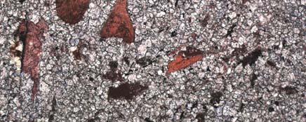
164 Sample 42 (Dolomitic fossiliferous limestone) Sample 44 (Fossiliferous calcareous dolomite) Sample 48 (Micritic dolostone) 147

165 Sample 61 (Fossiliferous limestone) (Note: SEM image incorrectly labeled as A10) Sample 62 (Fossiliferous limestone) Sample 64 (Fossiliferous dolomitic limestone) 148

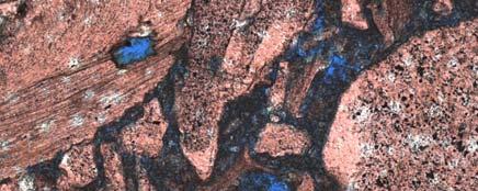
166 Sample 69 (Dolostone) (Note: SEM image incorrectly labeled as A10) Sample 70 (Dolostone) Sample 71 (Fossiliferous limestone) 149

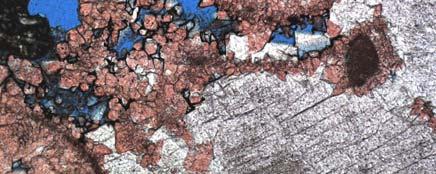
167 Sample 72 (Sandy fossiliferous limestone) Sample A10 (Micritic fossiliferous limestone) Sample A24 (Pelletal limestone) (Note: SEM image incorrectly labeled as A10) 150

168 APPENDIX F STATIC AND DYNAMIC MODULI DATA 151

169 152

170 APPENDIX G VRH AVERAGE CALCULATION Calculation of Voigt-Ruess-Hill Young s modulus for limestone and dolomite using the average mineralogy. The Young s moduli for various mineral components were calculated using the data available in Mavko et al. (1998) and Gomez (2007). 153

171 154