Study of the effects of magnetic field on the properties of combustion synthesized iron oxide nanoparticles

Transcription

1 Louisiana State University LSU Digital Commons LSU Master's Theses Graduate School 2005 Study of the effects of magnetic field on the properties of combustion synthesized iron oxide nanoparticles Nagaraju Komuravelli Louisiana State University and Agricultural and Mechanical College, Follow this and additional works at: Part of the Mechanical Engineering Commons Recommended Citation Komuravelli, Nagaraju, "Study of the effects of magnetic field on the properties of combustion synthesized iron oxide nanoparticles" (2005). LSU Master's Theses This Thesis is brought to you for free and open access by the Graduate School at LSU Digital Commons. It has been accepted for inclusion in LSU Master's Theses by an authorized graduate school editor of LSU Digital Commons. For more information, please contact

2 STUDY OF THE EFFECTS OF MAGNETIC FIELD ON THE PROPERTIES OF COMBUSTION SYNTHESIZED IRON OXIDE NANOPARTICLES A Thesis Submitted to the Graduate Faculty of the Louisiana State University and Agricultural and Mechanical College in partial fulfillment of the requirements for the degree of Master of Science in Mechanical Engineering In The Department of Mechanical Engineering By Komuravelli Nagaraju B.Tech, Jawaharlal Nehru Technological University, 2002 December, 2005

3 Dedicated To MY PARENTS and FAMILY ii

4 ACKNOWLEDGEMENTS First and foremost, I would like to thank my major professor Dr.Tryfon Charalampopoulos who has been instrumental in accomplishing my work. Without his guidance and teaching, this work would not have been possible. I sincerely thank him for his patience and technical insight in motivating me throughout this work. I would also like to thank Dr. Aravamudhan Raman and Dr. Wen Jin Meng, for spending their valuable time and lending their expertise in thoroughly reviewing my thesis. I also thank Dr. Mendrella, ECE department, Louisiana State University for his valuable suggestions which helped to further proceed during my research work. I thank Dr. Jiang for helping me in performing TEM and XPS analyses in Material Characterization Center, Louisiana State University. I express my sincere gratitude to my parents and my wife for their continuous support in all aspects. I would like to have the same kind of motivation and support from them forever. I also thank Dr. Young, Dr. Ditusa, Mr. Randy, Department of Physics, Louisiana State University, for all the help they provided during my research work. I am very thankful to all my roommates, Dinesh, Vijay, Sachin, Susheel and Naveed who have been my family here and lent me their unconditional support. Last but not the least, I would like to acknowledge my lab mates and my friends at LSU who made my stay memorable and enjoyable. iii

5 TABLE OF CONTENTS DEDICATION.... ii ACKNOWLEDGEMENTS.. iii LIST OF TABLES vii LIST OF FIGURES.. viii LIST OF SYMBOLS xii ABSTRACT.. xv CHAPTER 1. INTRODUCTION Summary Need for Studying the Morphology of Particulates Measurement Techniques and Methodology Proposed Work CHAPTER 2. LITERATURE SURVEY Generation of Chain like Nanoparticles by Iron-pentacarbonyl Induced Flames Characterization of Aggregates Magnetism and Types Diamagnetism Paramagnetism Ferromagnetism Antiferromagnetism Ferrimagnetism Properties of Magnetic Materials Hysteresis Magnetic characterization of nanoparticles Effects of particle size on magnetic properties CHAPTER 3. EXPERIMENTAL FACILITIES Burner Supply Feeding System Gas supply Additive feeding Electro-Magnet Thermophoretic Sampling System Positioning System Probe positioning Positioning of the thermocouple iv

6 CHAPTER 4. EXPERIMENTAL PROCEDURES Calibration Calibration of Ironpentacarbonyl mass flowrate Calibration of pneumatic actuator system Flames and Temperature Measurements The flames Temperature measurements Monitoring of Fe(CO) 5 Mass Flow Rate Particle Sampling Thermophoretic sampling Electromagnet CHAPTER 5. RESULTS AND DISCUSSION Samples from Thermophoretic Sampling Effect of Magnetic field on Diffusion Flames XPS Analysis Analysis of Magnetic Properties of Iron Oxide Nanoparticles using SQUID 65 CHAPTER 6. SUMMARY OF RESULTS REFERENCES.. 72 APPENDICES A. Properties of Iron Pentacarbonyl A.1 Physical data A.2 Safety data B. Values of Magnetic Field at Different Locations in the Air Gap C. Magnetic Force Acting on a Gas Group C.1 Force due to a magnetic field C.2 Field produced by the chain aggregates C.3 Faraday s law C.3.1 Inductance. 83 C.3.2 Calculation of L 84 C.3.3 How L is derived.. 85 D. Hysteresis Curves. 88 E. Samples Taken at Various Conditions E.1 Samples taken at various cylinder temperatures E.2 Samples taken at various flow rates of Fe(CO) E.3 Samples taken at various heights above the burner surface.. 93 F. TEM Micrographs of Samples Taken at Conditions shown in Table G. More TEM Micrographs of Samples at Various Cylinder Temperatures v

7 H. Magnetic Recording. 99 H.1 Magnetic recording - An introduction H.2 Recording H.3 Reading H.4 A Prototypical tape system H.5 The Media H.5.1 Particulate media H.5.2 Film deposition H.6 Recorders H.6.1 Open reel (reel-to-reel) recorders. 110 H.6.2 Cassette recorders I. Magnetic Effects of Iron Compounds on Binding Energy VITA 118 vi

8 LIST OF TABLES 1. Summary of various studies on Nano sized aggregates Summary of different types of Magnetic behavior Summary of various studies on Magnetic characterization of Nanoparticles Sampling conditions I Sampling conditions II Sampling conditions III Temperature values at different axial locations taken at 55 C cylinder temperature and 35/450 cc/min flowrate Forces developed due to Magnetic field around the Diffusion flame for different field values Magnetic parameters of the samples taken at different conditions Typical ranges for Magnetic properties in various storage devices vii

9 LIST OF FIGURES Figure.1.1 Structures of chain-like aggregates... 3 Figure1.2 Structure of a Hexagonally Closely Packed (HCP) single Nano crystal. 4 Figure 2.1 Atomic / Magnetic behavior of diamagnetic materials.. 14 Figure 2.2 Atomic / Magnetic behavior of paramagnetic materials Figure 2.3 Atomic / Magnetic behavior of ferromagnetic materials 17 Figure 2.4 Atomic / Magnetic behavior of antiferromagnetic materials. 18 Figure 2.5 Figure 3.1 Atomic / Magnetic behavior of ferrimagnetic materials.19 Experimental set up for the synthesis of chain like aggregates.. 28 Figure 3.2 Gas supply system. 30 Figure 3.3 Additive-feeding system 32 Figure 3.4 Pneumatic actuator and thermophoretic sampling system Figure 4.1 Set up for the calibration system Figure 4.2 Calibrated mass flowrate of Iron Pentacarbonyl at 25 C cylinder temperature.. 40 Figure 4.3 Electromagnet around the burner tube Figure 4.4 Axial temperature measurements for CO/air Diffusion flames at various heights above the burner surface at 450 cc/min of CO Figure 4.5 Magnetic lines of force at different locations in the air gap Figure 4.6 View of the electromagnet designed Figure 4.7 View of the thermophoretic sampling system viii

10 Figure 5.1 TEM Micrograph: sample taken at 10mm height above the burner surface with total flowrate of 450 cc/min and carrier flow rate of 35 cc/min at the cylinder temperature of 45 C without any Magnetic field around the CO/air Diffusion flame Figure 5.2 Figure 5.3 TEM Micrograph: sample taken at 10mm height above the burner surface with total flowrate of 450 cc/min and carrier flow rate of 35 cc/min at the cylinder temperature of 45 C with a Magnetic field of 0.4 Tesla around the CO/air Diffusion flame 55 TEM Micrograph: sample taken at 10mm height above the burner surface with total flowrate of 450 cc/min and carrier flow rate of 35 cc/min at the cylinder temperature of 45 C with a Magnetic field of 0.4 Tesla around the CO/air Diffusion flame 56 Figure 5.4 CO- room air Diffusion flame images at different velocities 58 Figure 5.5 Figure 5.6 Figure 5.7 Figure 5.8 Figure 6.1 Effect of the flame temperature on Inhomogeneous fields as a function of position from the burner surface XPS spectrum of an Iron Oxide Nanoparticles sample taken at 450 cc/min CO, 35 cc/min Fe(CO) 5 and at 10mm above the burner surface with and without Magnetic field High resolution spectra of Fe-2p and O-1s with and without Magnetic field.. 64 Variation of magnetization vs. temperature at different conditions. 66 Hysteresis curve of a sample taken at 50nm.70 Figure C.1 Schematic representation of Faraday s law.. 82 Figure C.2 Forces acting in a current coil.. 85 Figure C.3 Mechanical work done in a current coil.. 87 Figure D.1 Hysteresis curves of the samples taken at10nm, 35 C cylinder temperature, 10mm above burner surface ix

11 Figure E.1 Figure E.2 Figure E.3 Figure E.4 Figure E.5 Figure E.6 Figure E.7 Figure E.8 Figure E.9 Figure E.10 Figure E.11 Figure E.12 Figure F.1 Samples collected at a fixed flowrate 35/450 cc/min at 20 mm height with and without Magnetic field at 23 C cylinder temperature 89 Samples collected at a fixed flowrate 35/450 cc/min at 20 mm height with and without Magnetic field at 35 C cylinder temperature 89 Samples collected at a fixed flowrate 35/450 cc/min at 20 mm height with and without Magnetic field at 45 C cylinder temperature 90 Samples collected at a fixed flowrate 35/450 cc/min at 20 mm height with and without Magnetic field at 55 C cylinder temperature 90 Samples collected at a fixed cylinder temperature of 35 C at 20 mm height with and without Magnetic field at a flow rate of 450cc/min CO and 25cc/min Fe(CO) Samples collected at a fixed cylinder temperature of 35 C at 20 mm height with and without Magnetic field at a flow rate of 450cc/min CO and 35cc/min Fe(CO) Samples collected at a fixed cylinder temperature of 35 C at 20 mm height with and without Magnetic field at a flow rate of 450cc/min CO and 45cc/min Fe(CO) Samples collected at a fixed cylinder temperature of 35 C at 20 mm height with and without Magnetic field at a flow rate of 450cc/min CO and 55cc/min Fe(CO) 5 92 Samples collected at a fixed cylinder temperature of 35 C at a flow rate of 450cc/min CO and 35cc/min Fe(CO) 5 at 12 mm height with and without Magnetic field 93 Samples collected at a fixed cylinder temperature of 35 C at a flow rate of 450cc/min CO and 35cc/min Fe(CO) 5 at 20mm height with and without Magnetic field 93 Samples collected at a fixed cylinder temperature of 35 C at a flow rate of 450cc/min CO and 35cc/min Fe(CO) 5 at 30mm height with and without Magnetic field 94 Samples collected at a fixed cylinder temperature of 35 C at a flow rate of 450cc/min CO and 35cc/min fe(co) 5 at 36mm height with and without Magnetic field 94 Samples of 10nm collected at 35 C cylinder temperature, 10mm above burner surface 450cc/min CO and 20cc/min Fe(CO) 5 95 x

12 Figure F.2 Figure F.3 Figure F.4 Figure F.5 Figure G.1 Figure G.2 Samples of 20nm collected at 35 C cylinder temperature, 16mm above burner surface 450cc/min CO and 25cc/min Fe(CO) 5 95 Samples of 50nm collected at 35 C cylinder temperature, 10mm above burner surface 450cc/min CO and 35cc/min Fe(CO) 5 96 Samples of 20nm collected at 45 C cylinder temperature, 10mm above burner surface 450cc/min CO and 35cc/min Fe(CO) 5 96 Samples of 50nm collected at 45 C cylinder temperature, 10mm above burner surface 450cc/min CO and 45cc/min Fe(CO) 5 97 Samples collected at 35 C cylinder temperature, 10mm above burner surface 450cc/min CO and 55cc/min Fe(CO) Samples collected at 45 C cylinder temperature, 10mm above burner surface 450cc/min CO and 55cc/min Fe(CO) Figure H.1 Example of a hysteresis plot of a gamma Ferric Oxide sample 99 Figure H.2 Simple recording system Figure H.3 Variation of analog signal in recording. 101 Figure H.4 A simple reading system 102 Figure H.5 A typical tape system Figure H.6 Particulate Magnetic media 105 Figure H.7 Typical Magnetic materials 105 Figure H.8 Plating technique to create metal films Figure H.9 Thermal evaporation technique Figure H.10 E-Beam evaporation technique Figure H.11 DC and RF sputtering. 110 Figure H.12 Reel-to-Reel tape recorder system Figure H.13 Typical cassette recorders Figure I.1 Magnetic moment and angular momentum xi

13 LIST OF SYMBOLS χ χ o H M B C T θ T c T N susceptibility of gas group susceptibility of air applied magnetic field magnetization of a material magnetic field at different locations in air gap Curie constant temperature temperature constant Curie temperature Neel temperature y mass flow rate of Fe(CO) 5 x R F G T i k p m mass flow rate of CO distance from one end of the magneto the center of air gap magnetic force acting on the gas group gauss tesla current boltzmann constant dipole moment N number of atoms in a unit volume f fraction of dipole moments µ o permeability of free space xii

14 µ permeability of the material W l d m a E φ t L q U energy stored in magnetic matter differential length of the chain aggregate diameter of a single spherical particle moment of a chain aggregate aspect ratio electric field magnetic flux time inductance charge total magnetic energy stored in the magnetic material R resistance of the rectangular current coil N F 1, F 2 B 1, B 2 Φ 12 V number of turns of the rectangular current carrying coil forces acting from both ends of the rectangular current carrying coil magnetic field acting at both ends of the rectangular current carrying coil magnetic flux that flows from first end of the coil to the second end of coil velocity f frequency of the analog signal in a reading system e induced voltage F magnetic surface flux in a simple reading system r orbit radius xiii

15 c j q p h λ U velocity of light angular momentum force on a moving charge de Broglie s momentum Planck s constant wavelength energy function xiv

16 ABSTRACT Nanosized chain-like aggregates were developed in an iron pentacarbonyl-carbon monoxide (Fe(CO) 5 CO) air diffusion flame system. Magnetic field was applied around the diffusion flame using an electromagnet with an intensity of 0.4 Tesla. Transmission Electron Microscopy (TEM) analysis was performed to observe the behavior of the chains formed and to study the effect of magnetic field on these chains. These chain aggregates consist mainly of Fe 2 O 3, which play a vital role in magnetic storage devices. X-ray Photon Spectroscopy (XPS) were carried out to confirm that the chain aggregates consist of mainly γ-fe 2 O 3. The effect of magnetic field on diffusion flames was observed clearly and the color of the flame also became brighter indicating the increase in the flame intensity. The temperature increase at different locations in the flame was between C. The effects of the application of external magnetic field on Fe(CO) 5 CO air diffusion flame were studied. The magnetic properties of the iron oxide particles formed were investigated using a Super-conducting Quantum Interference Device (SQUID) magnetometer. It was observed that the magnetic properties such as coercivity, susceptibility and permeability favor the formation of oxides that can be used in magnetic storage devices when a magnetic field was applied. xv

17 Chapter 1. Introduction 1.1 Summary Nowadays a wide variety of particulate commodities are made by flame technology. The advantages of flame technology include flexibility, product quality, cleanliness and low capitol cost. The generated particulates possess various shapes such as random aggregates, cluster like, and chain-like structures. Study of nanosized chain-like aggregates and their formation mechanisms in chemically reacting systems such as flames is badly needed in research and practical applications. Information about the size and shape of particulates is critical in predicting the growth and oxidation of particulates in the combustion systems. It is also important in the synthesis of materials such as ceramics using the aerosol route, in engines, incinerators and boilers for efficient pollution control. Also, the knowledge of the chain - like aggregates is useful in many practical areas such as superconducting materials, magnetic storage devices, multi phase systems, vapor deposition studies and bio-medical applications. The present study focuses on the generation of chain-like aggregates consisting of spherical primary nanoparticles through combustion synthesis and the effect of magnetic field on these aggregates formed by diffusion flames. These aggregates were characterized in an iron pentacarbonyl-carbon monoxide (Fe(CO) 5 CO) air diffusion flame system without the application of external magnetic field [1]. X-ray diffraction measurements were used to identify the chemical states of the particulate components. The results indicated that the aggregates formed in this flame consisted predominantly of primary particles of iron oxide (Fe 2 O 3 ). In addition various iron oxides like Fe 3 O 4 and FeO were also formed. 1

18 This thesis is organized as follows. In this Chapter, the need for accurate knowledge of the effects of magnetic field on size and morphology of primary particles and their agglomerates are discussed and the proposed work is presented. In Chapter 2, previous works on the subject are reviewed, pointing to the need for further study on the subject. Chapter 3 deals with the experimental set up and the detailed procedures for the experimental measurements. Chapter 4 discusses the methods for collecting the samples, the calibration processes, sampling techniques and the calculations for the magnetic field. In Chapter 5 the results are analyzed and discussed. The study is concluded in Chapter 6 by putting forth the outcomes of the work, and the summary of the results as well as recommendations for future work. 1.2 Need for Studying the Morphology of Particulates It has been observed that the variation in the morphology and properties is a distinct characteristic of flame-synthesized particles [2, 3] when they are used in various applications such as the magnetic storage devices, bio-medical applications and industrial applications. Several areas of particulate formation require precise determination of the particle size in the sub-micron range as well as morphology. For example, it has been found that in the case of silica formed in flames, the measured growth rates for the particles extracted from the flames (as determined by the nitrogen absorption method) were two orders of magnitude slower than the model predictions. This is especially true at early stages of particle formation under flame conditions where the self-preserving size distribution breaks down. Knowledge of the initial distribution function is significant for two reasons [4]: 2

19 (i) (ii) For proper inversion of optical data; and For relating process variables such as feedstock and flow rates with the product quality [2]. The particulates composed of approximately spherical nanosized units are called aggregates, whereas the basic spherical units are referred to as primary particles. Because of Brownian motion and high number density of the units, typically ranging from 3x10 9 to 4x10 12 particles/cm 3 [1] gas for additive-doped flames, the primary particles generally do not exist individually in the flame; rather they coagulate into various types of aggregates. The aggregates produced by the flames could be of variable structures such as clustered, chain-like as shown in Fig. 1.1 and randomly structured aggregates. Figure1.1: Structures of chain-like aggregates [5] Chain-like aggregates are frequently observed in emissions of engines and other combustion systems like burners, furnaces, generators, and these systems have generated significant interest for their particularly structured shapes and their optical and radiative 3

20 properties. The properties of various types of particles formed were observed to be different. As such the focus of this study is on the chain like aggregates, as they are used in research and practical areas [6]. An example of a single Hexagonally Closely Packed (HCP) nano crystal in an Iron Oxide (FeO) chain-like aggregate, viewed in the isometric view, is shown in Fig Figure1.2: Structure of a Hexagonally Closely Packed (HCP) Iron Oxide single Nano crystal [7] The complete characterization of particulates including the distribution of particle size, number density of primary particles and the diameter of primary particles per aggregate as well as their optical properties were carried out in previous studies [4, 5]. 4

21 1.3 Measurement Techniques and Methodology Two techniques have been used to characterize nanoparticles in flames: in-situ and ex-situ. The in-situ optical technique has been proven powerful to yield particle size and morphology information. The in-situ light scattering approach yields accurate agglomerate parameters of particulates. However, this technique requires accurate knowledge of refractive index and is very sensitive to the structure of the aggregates, which is typically unknown in flame systems [1-6]. The structure of aggregates formed strongly depends on the operating conditions, which lead to difficulties in data interpretation. Hence, ex-situ techniques were used to collect and characterize particles in this study. Ex-situ technique is a different process compared to in-situ technique. In this method, particles are collected iso-kinetically. Samples for transmission electron microscopy are supported on a thin electron transparent film, to hold the specimen in place while in the objective lens of the TEM. Only samples that are self - supporting do not need some additional support film. The particles formed here are in the form of aggregates and so they are not self-supporting [8]. For this particular application 200-mesh carbon coated copper grids were selected as support films for samples, as copper is not attracted by magnetic field and external analysis was carried out. Particles are again collected on these grids in the presence of magnetic field. TEM is also employed with the ex-situ technique in which, information about the size and shape of the aggregates can be obtained. Sample preparation in TEM analysis is very time consuming which is overcome by this technique, wherein the samples are directly obtained on the grids, which can be analyzed by TEM. Information about the size, variation of aspect ratio with respect to the 5

22 concentration of additive added to the primary fuel in different flames and the evaporator cylinder temperatures, can be obtained by particle sampling. Furthermore, the particles collected with and without magnetic field are analyzed using a SQUID (Super-conducting Quantum Interference Device) magnetometer (See Chapter 3 for description), which shows the variation of magnetic properties as function of flow rates of Fe(CO) 5 and at different positions in the flame. 1.4 Proposed Work The purpose of the present study is to characterize and study the properties of the chain like aggregates collected with and without the application of a dc external magnetic field. Toward this end, the ex-situ technique was employed for the extraction of samples. Aggregates were withdrawn with sampling probes. The samples were collected on carbon-coated copper grids for TEM analysis and magnetic property analysis, and the agglomerate parameters were determined. The temperatures at which chain aggregates were formed were monitored using platinum vs. platinum-10% rhodium(pt vs Pt - 10% Rh) thermocouple probe. The selection of this particular flame system and fuel/oxidizer combination is justified since the primary particles formed in this type of flame have a natural tendency to form linear strings of aggregates [6]. An electromagnet was designed which generated a dc field ranging between 1.1 Tesla (T) to 1.5 T, which would exert an effect on the shape and structure of the diffusion flame. The value of the field was selected based on the results of previous works on the effects of magnetic field on diffusion flame structures [9-13]. The fields used earlier were 6

23 much higher than the field used in our study. Various researchers used different fields ranging from T. The results and discussions are presented in Chapter 5. 7

24 Chapter 2. Literature Survey In this Chapter, the formation of nanoparticles and chain like aggregates in flames, their morphological characteristics, effect of magnetic field on flames and magnetic properties of iron oxide nanoparticles are discussed. 2.1 Generation of Chain like Nanoparticles by Iron-pentacarbonyl Induced Flames The formation of iron oxides was studied previously in this laboratory by zhang [1]. Iron oxide nanoparticles (maghemite and magnetite) were formed by thermal decomposition of Fe(CO) 5 in the presence of residual oxygen of the system and by consecutive aeration. TEM analysis yielded primary particle sizes, aspect ratio and fuel feed rate, temperature of evaporation as function of vertical position in the flame. Recently [2, 3], chain-like aggregates were synthesized via the gaseous phase. This approach entails the use of specific fuel additives such as iron pentacarbonyl vapor. Here the additive fuels are heated to their evaporating temperatures, and are introduced into a flame for further decomposition and chemical reactions. The metal oxide vapors formed through this process subsequently nucleate and condense to form primary particles. Welldefined shapes of the aggregates were obtained by controlling the combustion parameters. The production of chain-like aggregate particles was attempted in 1958 by an exploding metal wire method, giving branched chains [14]. Chain-like aggregates were generated by exploding a copper wire of known diameter. Primary particles of uniform diameter were obtained by this method. The chain-like aggregates were stored in this method and as a result, distortions of the aggregate configuration were observed. This 8

25 was a major disadvantage of the process. Also controlling the process to produce uniformly dispersed chains was a difficult task. Herzer et al. [15] annealed amorphous ribbons of iron alloys to produce α-iron of ultra fine grain structures. The temperature dependence of these structures revealed two different magnetic phases corresponding to grains and grain boundary phases. These structures were nanocrystalline and exhibited excellent soft magnetic properties, which are widely used in storage devices. Bogdan et al. [16] performed an experiment to find the effect of crystallographic orientation on grain size distribution. The control of grain size statistics is essential in the manufacture of granular thin films used in high-density recording. Cobalt and Nickel alloy layer structures were analyzed. These layers act as magnetic layer and soft under layer respectively to distinguish between grains and grain boundaries. Images of the magnetic layer were observed with HRTEM (High Resolution TEM) images. The grain size distribution was determined using a high number of layers per sample and the boundary maps were obtained manually by tracing out the grain boundaries on the lattice image. The crystallographic orientation of magnetic layer was determined by epitaxial matching with nickel layer. The higher symmetry of magnetic layer increases grain size dispersion, which is required for magnetic recording. Kameda [17], using computer programs, found that the nanostructured metallic and ceramic materials have unique mechanical and magnetic properties. Nanostructured magnetic materials have been successfully fabricated during the past decade using an amorphous precursor processing method. During this process, partial and full transformations of amorphous precursors were prepared by melt spinning into nanocrystalline phases without introducing impurities and defects. This method is a viable route to develop soft 9

26 and hard magnetic nanostructured materials. The advantage of this method is the consolidation of mechanically alloyed powders and heavy deformation that yield impurity precipitation and structural defects. Bean et al. [18] found that the magnetic technique of particle size measurement was based on the observed magnetization curve for an appropriate system of ferromagnetic particles. When a magnetic field is applied to a suspension of small ferromagnetic particles, they are partially aligned by the field, and partially disordered by thermal motion, thereby exhibiting an overall paramagnetism. Single domain particles were treated as giant molecules to deduce the magnetic moment per particle and hence the particle size. The average magnetic moment per particle was obtained from this analysis and the average particle size was then determined. From this method sizes of ferromagnetic particles in the range from 20A-100A were easily measured, but particles smaller in diameter could not be measured. The magnetic granulometry method is firmly grounded and is capable of wider applicability. In this study, nanoparticles were produced in the author s laboratory by combustion synthesis and the effects of external magnetic field on particles magnetic properties are determined. The studies discussed above are summarized and shown in Table Characterization of Aggregates Various studies have been carried out for characterizing nanoparticles formed in combustion processes. The chain concept of aggregates was first given by Cohan and Watson [19] by TEM. The shape of the carbon black aggregates formed in their processes revealed considerable information about the structure of aggregates. This provided the basis for the analysis of structural characterization of aggregates by various Electron Microscopy processes. 10

27 Table 1: Summary of various studies on Nanosized aggregates Author / Year Chace and Moore / 1953 Bean et.al / 1954 Herzer et. al / 1990 Charalampopoulos / 1993 Z.Zhang & Charalampopoulos / 1995 Bogdan et. al / 2002 Kameda et. al / 2005 Experiment Technique Exploded Copper wire Method Magnetic field was applied to suspension of small ferromagnetic particles Annealing of amorphous ribbons of iron alloys Use of Fe(CO) 5 as additive fuel along with diffusion flame CO-air diffusion flame Device which gives effect of crystallographic orientation on grain size distribution on different materials Numerical programs Type of Particles Formed Chain like Aggregates Particles in order of Angstroms α-iron of ultra fine grain structure Nanosized aggregates were formed Nano-particles were formed Different grains and grain boundaries were observed Result Aggregates were formed with uniform diameter Magnetic moments of particles were obtained Nanocrystalline structures of iron were formed Well defined shapes were obtained by controlling combustion parameters Aspect ratio distributions, size and morphology distributions Different orientations of grains were observed - Nanoparticles have unique mechanical and magnetic properties Comments Aggregates need to be stored for use which resulted in distortions Nanoparticles were not able to be suspended Excellent soft magnetic properties were observed which were used in magnetic storage devices Further analysis is being done for this type of particles Nanoparticles were formed which gave an idea for further analysis of properties Helps in Manufacture of granular thin films Properties of nanosized magnetic materials and ceramic materials were obtained It was found that the morphological analysis of different grades of carbon black provided reasonable results regarding the distribution of aggregate sizes. This study gives a better understanding of the mechanism of formation of the aggregates. Later many researchers specifically studied the size distribution, aspect ratio distribution and distribution of numbers of aggregates formed by combustion processes, 11

28 but found that the particles are large in diameter and had broad coverage range. The results obtained did not reflect the complete formation of properties within the flame. 2.3 Magnetism and Types In this section, a brief account of the magnetic properties of materials is provided. All materials can be classified in terms of their magnetic behavior falling into one of five categories depending on their bulk magnetic susceptibility. Susceptibility is a measure of the degree to which a substance may be magnetized. It is defined as the ratio of the intensity of the induced magnetization I (Tesla) to the causative magnetic field H (Tesla) i.e., Magnetization Susceptibi lity, χ = Eqn (1) MagneticField Susceptibility has been shown to be proportional to the volume percentage of magnetic material contained in a medium. The two most common types of magnetism are diamagnetism and paramagnetism, which account for the magnetic properties of most of the elements of the periodic Table at room temperature. Such elements are usually referred to as non-magnetic, whereas those, which are referred to as magnetic, are actually classified as ferromagnetic. The only other type of magnetism observed in pure elements at room temperature is antiferromagnetism. Magnetic materials can also be classified as ferrimagnetic although this is not observed in any pure element but can only be found in compounds, such as the mixed oxides, known as ferrites, from which ferrimagnetism derives its name. The value of magnetic susceptibility falls into a 12

29 particular range for each type of material and this is shown in Table 2 with some examples. Table 2: Summary of different types of Magnetic behavior [20] Type of Magnetism Susceptibility Atomic/Magnetic Behavior Diamagnetism Small & Negative Atoms have no magnetic moment Paramagnetism Small & Positive Atoms have randomly oriented magnetic moment Ferromagnetism Large & positive, function of applied field, microstructure dependent Atoms have parallel aligned magnetic moments Antiferromagnetism Small & Positive Atoms have mixed parallel and antiparallel aligned magnetic moments Example/Susceptibility Au/χ * 10-6 Cu/χ *10-6 β-sn/χ Pt/χ * 10-6 Mn/χ * 10-6 Fe/χ ~ 100,000 Cr/χ * 10-6 Ferrimagnetism Large & positive, function of applied field, microstructure dependent Atoms have antiparallel aligned magnetic moments Ba/χ ~ Diamagnetism In a diamagnetic material the atoms have no net magnetic moment when there is no applied field. Under the influence of an applied field (H) the spinning electrons precess and this motion, which is a type of electric current, produces a magnetization (M) in the opposite direction to that of the applied field. This is the reason behind the negative susceptibility of diamagnetic materials as shown in Fig All materials have a diamagnetic effect; however, it is often the case that the diamagnetic effect is masked by 13

30 the larger paramagnetic or ferromagnetic term. The value of susceptibility is independent of temperature. The magnetic behavior of diamagnetic materials is as shown in Fig M H Figure 2.1: Atomic / Magnetic behavior of diamagnetic materials [8] Paramagnetism There are several theories of paramagnetism, which are valid for specific types of material. The Langevin model, which is true for materials with non-interacting localized electrons, states that each atom has a magnetic moment, which is randomly oriented as a result of thermal agitation. The application of a magnetic field creates a slight alignment of these moments (as shown in Fig.2.2) and hence a low magnetization in the same direction as the applied field. M H Figure 2.2: Atomic / Magnetic behavior of paramagnetic materials [8] 14

31 As the temperature increases, the thermal agitation will increase and it will become more difficult to align the atomic magnetic moments and hence the susceptibility will decrease. This behavior is known as the Curie law and is shown below in Eqn.2, where C is a material constant called the Curie constant [8]. C χ = T Eqn (2) Materials which obey this law are materials in which the magnetic moments are localized at the atomic or ionic sites and where there is no interaction between neighboring magnetic moments. The hydrated salts of the transition metals are examples of this type of behavior as the transition metal ions, which have a magnetic moment, are surrounded by a number of non-magnetic ions / atoms, which prevent interaction between neighboring magnetic moments. In fact the Curie law is a special case of the more general Curie-Weiss law (Eqn.3), which incorporates a temperature constant (θ) and derives from Weiss theory, proposed for ferromagnetic materials, that incorporates the interaction between magnetic moments [19]. C χ = T θ Eqn (3) In this equation θ can either be positive, negative or zero. Clearly when θ = 0 then the Curie-Weiss law equates to the Curie law. When θ is non-zero then there is an interaction between neighboring magnetic moments and the material is only paramagnetic above a certain transition temperature. If θ is positive then the material is ferromagnetic below the transition temperature and the value of θ corresponds to the transition temperature (Curie temperature, T C ). If θ is negative then the material is antiferromagnetic below the 15

32 transition temperature (Néel temperature, T N ), though, the value of θ does not relate to T N. It is important to note that this equation is only valid when the material is in a paramagnetic state. It is also not valid for many metals, as the electrons contributing to the magnetic moment are not localized. However, the law does apply to some metals, e.g. the rare earths, where the 4f electrons, that create the magnetic moment, are closely bound. The Pauli model of paramagnetism is true for a material where the electrons are free and interact to form conduction band. This model is valid for most paramagnetic metals. The Pauli paramagnetization value is used to obtain the theoretical value of susceptibility of magnetic materials. In this model the conduction electrons are considered essentially to be free and under an applied field an imbalance between electrons with opposite spin is set up leading to a low magnetization in the same direction as the applied field. The susceptibility is independent of temperature, although the electronic band structure may be affected, which will then have an effect on the susceptibility Ferromagnetism Ferromagnetism is only possible when atoms are arranged in a lattice and the atomic magnetic moments can interact to align parallel to each other. This effect is explained in classical theory by the presence of a molecular field within the ferromagnetic material, which was first postulated by Weiss in This field is sufficient to magnetize the material to saturation. In quantum mechanics, the Heisenberg model of ferromagnetism describes the parallel alignment of magnetic moments in terms of an exchange interaction between neighboring moments [20]. 16

33 Weiss postulated the presence of magnetic domains within the material, which are regions where the atomic magnetic moments are aligned (Fig. 2.3). The movement of these domains determines how the material responds to an external magnetic field and as a consequence the susceptibility is a function of the applied magnetic field strength. Therefore, ferromagnetic materials are usually compared in terms of saturation magnetization (magnetization when all domains are aligned) rather than susceptibility. In the Periodic Table of elements only Fe, Co and Ni are ferromagnetic at and above room temperature. As ferromagnetic materials are heated, the thermal agitation of the atoms implies that the degree of alignment of the atomic magnetic moments decreases and hence the saturation magnetization also decreases. Eventually the thermal agitation becomes so great that the material becomes paramagnetic; the temperature of this transition is the Curie temperature, T C (Fe: T C =770 C, Co: T C =1131 C and Ni: T C =358 C). Above the Curie temperature, T C, the susceptibility varies according to the Curie-Weiss law. M H Figure 2.3: Atomic / Magnetic behavior of ferromagnetic materials [8] 17

34 Figure 2.3 explains the typical behavior of ferromagnetic materials. When thermally agitated, the magnetization of the material increases until a certain value is reached i.e., the Curie temperature and behaves as a paramagnetic material when the temperature is further increased Antiferromagnetism In the periodic table the only element exhibiting antiferromagnetism at room temperature is chromium. Antiferromagnetic materials are very similar to ferromagnetic materials but the exchange interaction between neighboring atoms leads to the antiparallel alignment of the atomic magnetic moments (Figure 2.4). M H Figure 2.4: Atomic / Magnetic behavior of antiferromagnetic materials Therefore, the magnetic field cancels out and the material appears to behave in the same way as a paramagnetic material. Like ferromagnetic materials these materials become paramagnetic above a transition temperature, known as the Néel temperature, T N. (For Chromium, T N =37ºC) Ferrimagnetism Ferrimagnetism is only observed in compounds, which have more complex crystal structures than pure elements. Within these materials the exchange interactions lead to parallel alignment of atoms in some of the crystal sites and anti-parallel alignment of 18

35 others (Figure 2.5). The material breaks down into magnetic domains, just like a ferromagnetic material and the magnetic behavior is also very similar, although ferrimagnetic materials usually have lower saturation magnetizations. M H Figure 2.5: Atomic / Magnetic behavior of ferrimagnetic materials For example in Barium ferrite (BaO.6Fe 2 O 3 ) the unit cell contains 64 ions of which the barium and oxygen ions have no magnetic moment, 16 Fe 3+ ions have moments aligned parallel and 8 Fe 3+ aligned anti-parallel giving a net magnetization parallel to the applied field, but with a relatively low magnitude as only ⅛ of the total ions contribute to the net magnetization of the material [20]. 2.4 Properties of Magnetic Materials In discussing magnetic materials it is convenient to regard a magnetic field as giving rise to magnetic induction. The magnetic induction has two components, one due directly to the magnetic field and the other to the intensity of magnetization of the material M (Tesla) produced by the field. The Magnetization is related to the field strength H (Tesla) by the equation M = χh Eqn (4) where χ is the magnetic susceptibility of the material. 19

36 2.4.1 Hysteresis If an increased magnetizing field H is applied on an unmagnetised bar of a ferromagnetic substance and a curve of M vs. H is plotted, a point is reached beyond which the intensity of magnetization remains constant and is said to be saturated. Now if the magnetizing field is decreased gradually to zero, it is found that the intensity of magnetization instead of being zero has a certain value. This value of intensity of magnetization for which H=0, is called residual magnetism or remnant magnetization. Again a reverse magnetic field is applied to reduce a magnetically saturated structure from remanence to zero magnetic induction. This field value is called as the coercivity. In the whole process, there is a loss of energy in taking a magnet through a cycle, and it appears as heat in the specimen. The net work done in taking the specimen completely through a Hysteresis cycle equals the total area enclosed in the entire M-H loop [21]. Different magnetic materials have different values of coercivity and remnant magnetization values and hence the susceptibilities Magnetic characterization of nanoparticles Inhomogeneous magnetic fields have been found to promote combustion reactions in diffusion flames. This phenomenon was first observed by Faraday [22] in Faraday observed that when a magnetic field was applied, a candle flame distorted its shape forming of an equatorial disk. This formed the basis for the study of magnetic effects on diffusion flames. Recently, Wakayama [23] found that when a fuel gas flowed in the direction of decreasing field strength, the burning velocity was found to increase. A homogeneous magnetic field was generated in the central area of an electromagnet with a gradient field. Methane gas or a mixture of methane and air flowed through a glass pipe. 20

37 The effect of inhomogeneous magnetic fields was studied by measuring the flame temperature and the area of the flame front. The comparison of diffusion flames with and without magnetic field revealed that the flame became more brilliant immediately after the application of the field and returned to the original state after the removal of field. The flame temperature also increased rapidly when the field was turned on and returned to the original value when it was turned off. Wakayama also studied the magnetic effects on hydrogen flames by measuring the temperature and the absorption spectrum. It was found that the flame without a field appeared to be flat shaped. When the field was applied, the flame became blue and triangular and turned more brilliant. These observations led him to conclude that magnetic field also promoted combustion. Wakayama [24] also studied about the synthesis of materials under magnetic field and magnetic control of gas flow and promotion of combustion. A new kind of magnetic effect was introduced called the Magnetohydrodynamics. These effects have been widely used in the area of electromagnetic processing of materials. It was found that the magnetic attractive force acting on paramagnetic oxygen gas induces gas flows and affects combustion. From this study, it was inferred that strong magnetic fields provide a new environment to synthesize new materials Effects of particle size on magnetic properties The effect of particle size on magnetic properties of nano-crystalline γ-fe 2 O 3 has been studied [25] using a DC magnetization technique, as a function of temperature and magnetic field. A super paramagnetic-type blocking process is observed in the Zero-fieldcooled (ZFC) and field-cooled (FC) magnetization. The ZFC and FC magnetization curves, recorded under an applied magnetic field of 100 Oersted for all the three samples 21

38 showed irreversibility. In this process, nanocrystalline samples of γ-fe 2 O 3 were prepared using a reverse micelle technique. The nanoparticles of different average particle size were obtained by annealing the as-prepared sample at different temperatures. It was observed that Coercivity increased with increasing particle size, while the saturation magnetization decreased with increasing particle size. Large-scale production of the iron oxide nanoparticles with this process was observed to be very difficult, as it requires a lot of time. Characterization of iron oxide nanoparticles was carried out [26] in a Fe 2 O 3 -SiO 2 composite prepared by a sol-gel method. The composite was prepared by a gelation method that adopts tetraethoxysilane and iron (III) nitrate as starting materials. The dried gel was treated at increasing temperatures, and the samples were characterized by XRD (X ray diffraction), TEM and magnetic susceptibility measurements. Nanosized iron oxide (III) particles were observed in the samples treated at low temperature (~300 C). Also XRD and TEM exhibited the formation of γ-fe 2 O 3 crystalline particles, which were super paramagnetic in nature. At higher temperatures typically above 300 C, there was no increase in the particles sizes but in turn, there was a transition from antiferro magnetic behavior to ferrimagnetic behavior. Also, further increase in temperature gave rise to the formation of α-fe 2 O 3. Atomic reorganization also was seen during these transition periods. Synthesis of iron oxide (γ-fe 2 O 3 ) i.e., maghemite and magnetite nanoparticles was carried out [27] by thermal decomposition of Fe(CO) 5 in the presence of residual oxygen of the system and by consecutive aeration. The particles were investigated by HRTEM (High resolution TEM), XRD and Mossbauer spectroscopy. Fe(CO) 5 was injected into a 22

39 mixture containing octyl ether and oleic acid at a fixed temperature. The resulting mixture was slowly heated and refluxed. This process was repeated for different molar ratios (3.04mmol 6.08mmol) for obtaining maghemite and magnetite particles of various sizes. TEM analysis was done on samples prepared by depositing a drop of diluted nanoparticles solution in toluene on a carbon-coated copper grid and drying it naturally. Cu Kα radiation was used for obtaining XRD patterns. Mossbauer spectra were recorded using a constant-acceleration Mossbauer spectrometer in which the isomer shift values were reported with respect to the Fe metal. The magnetic data were obtained using a SQUID. SQUID (an acronym for Superconducting Quantum Interference Device) is based on the concepts of flux quantization and Josephson tunneling through a weak link. One of the functions of a SQUID is to make extremely sensitive measurements of magnetic fields. The SQUID used in this study can measure a magnetic moment with a range of sensitivity from 10-8 to 2 emu in the standard configuration and can measure over 300 emu. There are several varieties of SQUIDs in use in modern laboratories today. In this analysis MPMS-SQUID (Magnetic Property Measurement System SQUID) is being used which is a highly integrated instrument system, designed to be a primary research tool in the complicated study of magnetism in matter. TEM images revealed that the size of nanoparticles decreased as the molar ratio of oleic acid to Fe(CO) 5 increased. This observation was also made by Hyeon et al.[28]. The particle size of the nanoparticles showed a trivial change before and after aeration process. The XRD patterns showed that the aerated particles matched with those of maghemite and magnetite. The larger nanoparticles showed higher intensity and the narrower peak width. The repeated aeration and heating of magnetite evolved maghemite nanoparticles. 23

40 However, the repeated aeration and reflux could not convert maghemite to hematite (α- Fe 2 O 3 ), which is the most stable phase of iron thermodynamically [29]. The Moessbauer spectra represented the super paramagnetic property of the particles. Hysteresis curves were generated using SQUID magnetometer. The magnetization curves showed that the particles were increasing proportionately with temperature, which represented ferromagnetic behavior. The coercivity and remnance (will be discussed in the following Chapters) values from the magnetization curves of some particles were not discernible indicating that the particles were super paramagnetic. However, the future work of the aeration method was to produce particles using Thermophoretic sampling system through which particles were able to be formed in a large scale and were more distinctly collected without any disturbances. A system was also developed [30] to magnetically measure biological antigen antibody reactions with a SQUID magnetometer. Antibodies were labeled with magnetic nanoparticles of γ-fe 2 O 3, and the antigen-antibody reactions were measured by detecting the magnetic field from the magnetic nanoparticles. A set up was built which detected the nanoparticles by weight. Magnetic particles as small as 600 pg (picogram) were detected. However, the process has a very limited application to only antigen-antibody reactions. The various studies on magnetic characterization of nano particles are shown in Table 3. The system in this study uses carbon monoxide as the fuel into which iron pentacarbonyl (Fe (CO) 5 ) is seeded at a given flow rate. This system was designed to overcome the difficulties faced in various mentioned research works and to obtain more efficient and useful magnetic properties so that practical applications can be carried out in the future. Thermophoretic sampling system was used to collect iron oxide nanoparticles. 24

41 Table 3: Summary of various studies on Magnetic characterization of Nanoparticles Author / Year Faraday / 1847 Wakayama / 1993 Wakayama / 1997 Williams et al. / 1996 Ennas et al. / 1998 Mukadem et al. / 2004 Experiment Technique Magnetic Field around a candle flame Magnetic Field effects around methane-air diffusion flames Synthesis of materials obtained by applying magnetic field around diffusion flames Biological Antigen- Antibody reactions were performed using SQUID magnetometer Synthesis of materials using Solgel method DC Magnetization technique Woo et al. / 2004 Characterization by Thermal decomposition method & by consecutive aeration process Komuravelli / 2005 Magnetic characterization of particles formed by CO-air diffusion flame Particles Result Comments / characterized Limitations - Deflection of candle This experiment flame at high magnetic formed the basis fields for magnetic field effects on flames - Burning velocity of the Gradient field flame increased. Flame effects were became more brilliant studied and thinner when a field was applied Nanoparticles were formed Nanoparticles were formed - Magnetohydrodynamics (MHD) effects were observed Nanocrystalline particles were formed Nanoparticles were formed Nanoparticles were formed Hysteresis curves were obtained TEM & XRD analysis was carried out Zero Field Cooled (ZFC) and Field Cooled (FC) curves were obtained Hysteresis curves were obtained using SQUID TEM, XRD & SQUID analysis is being carried out Electromagnetic processing of materials was possible Limited application due to Antigen-Antibody reactions Large scale production of particles was difficult Synthesis would be better if particles were collected by Thermophoretic Sampling Thermophoretic sampling method is being used for sampling - Synthesis of the particles was done using HRTEM, XPS, EDS (electron diffraction spectroscopy) and SQUID magnetometer. The crystal structure, composition and magnetic properties of the particles were determined using these measurements which include coercivity, susceptibility and remnant magnetization. Particles were collected at different flow rates under the following conditions. The total flow rate [Fe(CO) 5 and CO] 25

42 was kept at 450 cc/min and the flow rate of Fe(CO) 5 was varied in the range of 25 cc/min to 55 cc/min. 26

43 Chapter 3. Experimental Facilities The magnetic effects on CO/air diffusion flame and the synthesis of chain-like aggregates were studied using a specifically designed experimental facility. The facilities designed and fabricated for this study enabled to study the properties of the aggregates formed. The experimental setup consists of following subsystems: electromagnet, additive feeding, sampling and driving mechanism, gas supply and burner. The particulates formed using this experimental setup were extracted and the properties were studied using available instrumentation in the LSU campus. The samples were examined under TEM. [JEOL, Model 2010 HRTEM]. This instrument provided high magnification to ensure the samples to be viewed very clearly. The resolution is as high as 250K, which is adequate to resolve the iron oxide particles from the background matrix of the sample collector [carbon coated Cu grid acts as the background here]. A SQUID magnetometer [Quantum Design] was used to analyze the magnetic properties of the samples. Hysteresis loops were generated using the SQUID and the coercivity and remnant magnetization, which are properties useful in soft magnetic material applications were calculated. A schematic of the chain like aggregate generator experimental set up is presented in Figure 3.1. The detailed descriptions of each subsystem are presented in this Chapter. 3.1 Burner A ¼ inch diameter stainless steel tube was used as a diffusion burner in this study. The fuel is directed from the gas supply to the surface of the burner through the tube, 27

44 whereas the atmospheric air acts as the oxidizer i.e., oxygen required for combustion is taken from the surrounding air. Pneumatic Actuator Adjustable Stand Honey Comb Stabilizer Solenoid Valve Oscilloscope Electromagnet Burner Battery Charger Figure 3.1: Experimental set up for the synthesis of chain like aggregates Three different burners were also tested during the early attempts to generate straight chain aggregates. The first burner tested by Zhang [5] was a multi-element flat flame diffusion burner supplied by Research Technologies [Model RD15]. The design of the burner prevents flame from flash back. However, during the preliminary test it was found that most fuel element tubes were blocked by particles through wall deposition. The second burner tested [5] was a water-cooled flat flame premixed burner, designed and constructed in the Laboratory. During the test, flashback occurred due to the elevated temperature in the rim of burner chamber, and the iron oxides clogged the honeycomb. The third burner used was a concentric tube diffusion burner. The burner had three concentric stainless steel (316) tubes. The fuel was directed to the surface of the burner through the central tube, whereas oxidizer is supplied through second outer annular tube and mixes with the fuel above the burner surface. Nitrogen gas is provided by the outer 28

45 most tube to prevent the surrounding air from diffusing into the flame. The diameter of the inner tube was ¼, and the annular interval between the tubes is 1/8. The aggregates were collected using this burner. The fuel used in this study was CO burning in atmospheric air and as such a concentric tube burner was not required. This set up was better suited to accommodate the electromagnet which was poisoned around the flame. 3.2 Supply Feeding System The supply-feeding system was designed to deliver fuel and purging gases into the burner. The amount of each gas flowing through the burner was controlled and monitored accurately using flow-meters and needle valves. Added to this, the system also is provided with a design to deliver oxidizer, dilution and shroud gases. Iron additive was mixed with carbon monoxide in the burner tube through this system. The description of the system is provided below Gas supply Figure 3.2 shows the gas supply system used to generate the Fe(CO) 5 - CO diffusion flame. The system is designed in such a way that the flow rate in each gas line can be varied with needle valves. Gases are supplied here from different gas tanks. Carbon monoxide gas is passed in one line and purging nitrogen is passed from a different gas tank to purge any gas line. In this system the flow rates of gases were regulated using different flow meters and flow regulators. The flow meters monitor the gas is flowing through the line and the regulators are used to control the flow of the gases. The gases used here, i.e., carbon monoxide and nitrogen, are a high purity grades [99%, supplied by Lincoln Big Three, Inc]. 29

46 Figure 3.2: Gas supply system The critical flow rate of carbon monoxide is controlled by a needle valve and it is monitored with a Brooks Rotameter [Emerson Electric Co., Series No /2]. Nitrogen is passed through the fuel line after each run so as to purge the line. The fuel additive (iron pentacarbonyl) flow rate is monitored by a thermal type digital gas flow meter [Hastings, Model HFM 200] with a fluctuation of less than ±2% of the full scale flow rate of 50 standard liters per minute (slpm). Since iron pentacarbonyl (Fe(CO) 5 ) is highly corrosive, the system supply lines were purged with nitrogen after each run to prevent the additive gas - line from corroding. In addition, the whole gas supply system, including the burner and digital flow meter, is purged with nitrogen after the burner is shut down to make sure that there are no deposits of the gas on the walls of the gas tube. 30

47 3.2.2 Additive feeding Iron pentacarbonyl was chosen as additive fuel along with CO. The choice of this additive was based on previous works that in this system, chain-like aggregates were formed. The property of Fe(CO) 5 is that it can be easily vaporized and carried by carrier gases like propane, carbon monoxide and nitrogen. It also decomposes very slowly in liquid phase under room temperature. Other properties of iron pentacarbonyl can be found in Appendix. A. In this set up the system is designed in such a way that the amount of iron pentacarbonyl vapor delivered to the main gas line can be known and is controllable. A stainless steel cylinder, with a 2.5-inch of diameter and 6-inch length, is used to hold the additive. It also is used as an evaporator. A fiberglass taped heating wire [Omegalux, Model FGH ] was wrapped around the cylinder as insulation. As a result, a constant pre-set temperature within the range of freezing point (-15ºC) and boiling point (103ºC) can be set. The temperature chosen here was in the range of 23ºC to 55ºC. A PID microprocessor controller [Omega, Model CN 9000] was employed to control the temperature of the vaporization cylinder to within ±1ºC. The method of adjusting and controlling the temperatures will be discussed in detail in the following Chapter. Carbon monoxide gas here functions as a carrier gas. The gas flows from the cylinder and part of it is by-passed from the main line so that it mixes with the column of liquid Fe(CO) 5 and bubbles the Fe(CO) 5 vapor. Further dilution of the mixture is achieved by the bulk CO flow, and it is directed to the surface of the burner for subsequent ignition. The amount of additive introduced into the main line is determined with a calibration procedure, which involves measuring the amounts of iron pentacarbonyl condensed for a given set of 31

48 conditions. A condensation coil is used to collect the condensed iron pentacarbonyl vapor. The schematic of the additive feeding system is shown in Figure 3.3. The calibration procedures are described in detail in the following Chapter. Figure 3.3: Additive - feeding system [5] The quantities of fuel additive and fuel need to be accurately monitored. As such, great care was exercised to prevent the deposition of Fe(CO) 5 on the inner surface of the line via condensation. Specifically, the whole fuel line from the downstream of evaporator cylinder is wrapped and heated with electrically insulated heating wire [ACE GLASS INC., Model 12065, yielding a maximum temperature of 594ºC]. The external surface of the heating tape is insulated thermally insulated with glass fiber insulator [LEWCO, Model FT60-2]. The main line temperatures are monitored by a thermometer [OMEGA, Model 115TC] at four different points along the line. A temperature controller [OMEGA, Model 6100] is used to maintain the main line temperature at 85ºC. As a result the condensation and deposition of the iron pentacarbonyl vapor on the inner walls of the line is minimized. 32

49 3.3 Electro-Magnet An electromagnet was designed to generate variable DC-magnetic fields for the study of magnetic field effects on diffusion flame and the properties of the aggregates. Previous studies revealed that a magnetic field in the range of T was required to deflect any diffusion flame [21 27]. A C-shaped electromagnet was designed for the application of magnetic field on the CO/air diffusion flame. A permanent magnet provided by the Department of Physics & Astronomy, LSU was converted to an electromagnet. The permanent magnetic field was measured to be 1530 Gauss and after converting, the magnet yielded values of magnetic intensity up to 4,000 Gauss. The main parts involved in building the electromagnet are iron core permanent magnet, battery charger, copper wire for winding and gaussmeter. The distance between the poles of the magnet is 5.2 cm. The field lines within the air gap were measured with a Gaussmeter [Model 475 Lake Shore Cryotronics, inc]. In order to increase the field strength the air gap was reduced to 3.0 cm. The field lines were plotted and they showed higher values of the field strength with 3.0 cm gap (see figure 4.5). Reducing the air gap further was not possible as it was difficult for the burner tube to be placed between the air gap. The process of measuring the field values is explained in the following chapter. The permanent magnet was converted to electromagnet by winding copper wire around each leg of the magnet. The power source used for the electromagnet was a 120/180 V DC battery charger [Schumacher Fleet Multi-Amp 180/200 amp starter charger, Electrical Engineering Department, LSU]. The current required to generate the required field was 20±2 amperes. The battery charger here was able to generate more than 20 amperes current. Two electrode clips of the battery charger were connected to the 33

50 ends of the 14 gauge copper-wires of the electromagnet. After switching the battery on, it was observed that the field enhanced considerably. A 14-gauge AWG wire was selected around each leg for the winding of the C-shaped permanent magnet. The material selected for the wire was copper with an electrical conductivity of 640 mho/m. 3.4 Thermophoretic Sampling System The thermophoretic sampling system designed and built in previous works [5] was used for the collection of particles in the present study on the carbon coated copper grids. A thermophoretic probe is provided so that it is attached to the pneumatic actuator and when the trigger is activated, the probe moves into the flame for a period of time ( milliseconds) The particle motion towards the cold surface of the collection grid is driven by the thermophoretic force acting on the (gas + particle) mixture and is proportional to the temperature gradient. The cold surface of this grid also quenches the reaction of particles that are deposited on the surface by virtue of the thermophoretic force. The advantage of using thermophoretic sampling is that, as opposed to other sampling processes, it eliminates the potential for further agglomeration of particles, The sampling system consists of a pneumatic cylinder, solenoid valve, and oscilloscope, which control the position and movement of the Thermophoretic probe. The system is shown in the Figure 3.4 The pneumatic used is a double acting pneumatic actuated cylinder [BIMBA, Model MRS-04-DXP] of ¾ diameter and 3 stroke. It is driven by an air pressure of 40 psi through an air-controlled directional 4-way solenoid valve [ASCO, Series 8017]. The calibration of the position and movement of the probe is carried out using a Hall effect 34

51 switch [BIMBA, Model HSC-09] mounted on the cylinder. A nitrile-based permanent magnet is mounted on the piston to operate the BIMBA Hall Effect (BHE) switch. Figure 3.4: Pneumatic actuator and thermophoretic sampling system [5] The switch is connected in series with a power supply and further to an oscilloscope so that the signal generated may be displayed and monitored. As such, the residence time of the thermophoretic probe in flame can be set a-priori. The output in the oscilloscope doesn t display any signal until the sensor is just above the magnet, which is present in the pneumatic cylinder. The principle followed here is that of Hall effect i.e., when a magnet is directly below any sensor, which senses any signals, there is a disturbance in the current distribution, which produces a potential difference across the output. The circuitry amplifies the potential difference and triggers the oscilloscope. The sampling system is designed so that a slight variation in time is sensed and is displayed in the oscilloscope screen. Also, by recording the position of the piston along with the 35

52 oscilloscope signal, the position of the probe and its movement is accurately determined. This is done in the process of calibration, which is described in the next Chapter. As discussed earlier, the thermophoretic probe is mounted on the piston shaft. The probe used in this sampling set up is a thin stainless steel strip with dimensions of 20mm X 4mm X 0.2 mm. It is also rigid enough to minimize any small vibration and also small enough to reduce the air circulation induced by the probe motion. The carbon coated copper grid [Electron Microscopy Sciences, Model CF200 Cu, 200 mesh] is placed on the tip of the probe and is taped manually on the edges using a high temperature fiberglass tape. The carbon-coated grids are selected because of their stability under any electron beam during the TEM or SQUID analysis. Compared with other coatings, Cu grids withstand relatively high temperatures [ K]. The exposure time is limited in the range of 250 to 360 milliseconds as it minimizes the oxidation of grids in the flame environment. The exposure time is also appropriate to avoid collection of significant number of particles which would render the discernment of aggregate morphology difficult. The four-way solenoid valve is triggered using a trigger switch in the valve control box, which sends a signal to the oscilloscope. The signal by the magnet is triggered by another relay switch so that the potential difference developed is seen in the oscilloscope. 3.5 Positioning System Probe positioning The position of the probe with respect to the burner surface is important in order to obtain reproducible measurements of the chain aggregates formed above the burner surface. The accurate positioning of the probe relative to the burner surface was 36

53 accomplished with the help of a vertical movement mechanism in which a roller is moved manually so that the movement is monitored using a ruler attached to it. Displacements as small as 0.5mm can be measured using this system. All the systems discussed above are placed on two rigid tables designed to withstand the load of each system. The tables were designed using solid works and the load analysis was done to check the bending moment induced by the load. The maximum load the table could withstand was found to be very high (4853 Newton) than that of the load of the systems used for the experiment Positioning of the thermocouple The thermocouple used for measuring temperatures was positioned above the burner surface within the flame using the positioning system described in Section above. Before using the thermocouple calibrations were done so that accurate measurements could be achieved. The detailed procedures of calibrations are explained in the next chapter. 37

54 Chapter 4. Experimental Procedures In this chapter, the detailed procedures followed for the measurements along with their calibrations are presented. 4.1 Calibration Calibration of Ironpentacarbonyl mass flowrate The calibration of the fuel additive system was carried out by measuring the condensed mass of iron pentacarbonyl vapor in a glass condensation coil. The calibration is carried by a carrier gas for a particular set of flow rates and time periods at fixed cylinder temperatures. A certain amount of Iron pentacarbonyl (200 ml) was taken in the vaporization cylinder maintained at 25±1 C. The procedure of calibration is as follows. Figure 4.1: Set up for the calibration system 38

55 Figure 4.1 shows the calibration system for the Fuel Additive. The calibration system was maintained at room temperature condition i.e., 25±1 C and was monitored with thermometer [Omega, Model 115TC]. The pyrex glass coil is the collecting coil initially filled with glass beads to increase the deposition surface area of condensing vapor. Before the calibration process the inner and outer surfaces of the tube are cleaned thoroughly with ethyl alcohol. The coil is then dried with compressed air and then immediately sealed with caps. The weight of the condensation coil is then taken on an analytical balance with an accuracy of 0.5mg [SCIENTECH, Model 5220]. Fe(CO) 5 freezes very fast at low temperature. So, the condensation tube was immersed in an ice bath filled with mixture of ethylene glycol and dry ice maintained at constant temperature, -15 C which is high enough to prevent Fe(CO) 5 from freezing and low enough to ensure the complete condensation of the vapor. The condensation coil was connected to the gas, CO, and the additive feeding system as shown in the previous chapter (Fig.3.3). The primary gas CO, is passed through the cylinder, carrying Fe(CO) 5 vapor out and passed through the by-pass line for about 5 10 minutes for establishing a constant flow rate. As soon as the steady state was reached a stop clock was switched on which had a predetermined time period around mins. As soon as the time limit was reached, the coil tube was disconnected from the system and was sealed again with the caps. The outer surface of the coil was then cleaned and dried thoroughly and the weight of the coil was noted. The difference of the two weights provided the total mass of Fe(CO) 5 deposited on the tube for a given flow rate and time period. Thus, the mass flow rate of iron pentacarbonyl vapor was determined. 39

56 Fig 4.2 shows the calibration curve. Each point in the calibration curve represents an average of three calibration runs with a maximum fluctuation of ±0.03 g/hr. Calibration of Fe(CO) 5 Fe(CO)5 (g/hr) y = 0.019x R 2 = mass flowrate Linear fit of mass flow rate carrier gas flow rate (cc/min) Figure 4.2: Calibrated mass flowrate of Iron Pentacarbonyl at 25 C cylinder temperature A linear least squares fit of the curve was y = 0.019*x Eqn (4.1) with a correlation coefficient of was obtained. Here in the equation 4.1, y represents the mass flow rate of iron pentacarbonyl an x represents the flow rate of carrier gas CO (cc/min) through the evaporator cylinder. The uncertainty may be due to fluctuation of temperature and the deposition of iron pentacarbonyl vapor on the line from cylinder to ice-bath. The carriage flow rates ranging from 20 cc/min to 100 cc/min correspond to Fe(CO) 5 mass flow rates produced by the fuel additive vaporization system from g/hr to g/hr with an accuracy of ±0.03 g/hr. The weights of the condensation coil before and after testing gases flowing through the system without iron 40

57 pentacarbonyl added in it should be identical. All the uncertainties are within the allowable measurement error range. The results are accurate as well as reproducible. Thus, the concentration of Fe(CO) 5 vapor seeded into the flame can be accurately controlled by adjusting the carrier gas flow rate Calibration of pneumatic actuator system The exposure time of the sampling grid to the flame and the transit time of the probe used to be controlled properly to avoid overlap of aggregates and the difficulties in data analysis were determined using a pneumatic actuator system. If the exposure time is longer during sampling, more particles are collected on the grid and the analysis becomes difficult. If the exposure time is short, very few particles are collected on the grid during sampling, which is not suitable for analysis. The exposure time of the probe to the flame environment is calculated by measuring the duration time of the piston at the end of the cylinder. The BHE switch is positioned at one end of the cylinder, while the magnet on the piston is on the other end. For a given pulse, the piston moves to the end of the cylinder where the switch is located and returns to its original position. The piston remains at the end of the cylinder for a predetermined time period. The oscilloscope generates a signal when the piston is located exactly below the switch. The trigger is generated by the potential difference caused by the magnet on the piston. The time measured here is the probe exposure time to the flame environment. By setting the pulse duration, the exposure time of the probe to the flame environment can be varied and also controlled. For the present work, the exposure time is in the range of 250 to 350 ms, depending on the sampling location and the concentration of iron pentacarbonyl seeded in the flame 41

58 The piston speed should be measured to determine the transit time of the probe to the flame. In this method, the BHE switch is mounted in the midpoint of the cylinder. For each trigger, the piston activates the switch twice while moving back and forth, and the oscilloscope records two sharp signals. The piston speed and the transit time can be determined by measuring the time interval between the peaks of the two signals and subtracting the piston duration time. The probe control system is calibrated to move the probe with a speed of m/s. An ideal probe control system is that which would instantaneously insert the Thermophoretic probe into the flame for a well-defined, controllable interval without causing any disturbance to the motion of the flame gases. The signals were checked repeatedly and reproducible probe paths were observed. 4.2 Flames and Temperature Measurements The flames In the present experiment, a carbon monoxide air diffusion flame was used for testing. It was observed that until a particular flow rate was reached, the flame was not steady. It was found to be sustaining for flowrates above 180 cc/min. When the flow rate increased to above 500 cc/min, the flame started becoming unstable, i.e., a flickering of the flame was observed and so it was not suitable for sampling. The CO flame seeded with iron pentacarbonyl was stable in the range of 210 to 450 cc/min. Tests showed that at a fuel flow rate of 450 cc/min, the size of the flame was suitable for investigation of particulate morphology. The electromagnet was placed around the diffusion flame as shown in Figure 4.3. The diffusion flames show different configurations at different flow rates. 42

59 Figure 4.3: Electromagnet around the burner tube When a fuel gas flowed in the direction of decreasing field strength, the burning velocity was found to increase. No magnetic effect was observed when the fuel gas flowed into homogeneous fields. The application of inhomogeneous fields promotes combustion reaction. It was observed that the flame became more brilliant after applying field and returned to the original state after the field was turned off. The flame temperature also increased. The effect of magnetic field on the CO/air diffusion flame used here can be clearly seen in the following Chapter Temperature measurements The temperature profiles of the carbon monoxide and room air diffusion flame were measured as function of the height of the burner surface for the diffusion flame. A k-type thermocouple was used with a bead diameter of 0.2 mm for measuring the temperatures. The thermocouple was placed on a translating mechanism, and was placed in the center of the burner surface. The flame measurements were measured for both flames i.e., with and without magnetic fields at a mass flow rate of 450 cc/min carbon monoxide. Figure 43

60 4.4 shows the variation of temperature with the height of the burner surface. It is also observed that when a magnetic field is applied the temperature increased. Axial Temperatures for CO/air Diffusion Flames at Various Heights above the burner surface with and without magnetic field Temperature (K) Temperature w/o field Temperature with field Axial Distances (mm) Figure 4.4: Axial temperature measurements for CO/air Diffusion flames at various heights above the burner surface at 450 cc/min of CO 4.3 Monitoring of Fe(CO) 5 Mass Flow Rate The additive mass flow rate is dependent on the flow rate of the carrier gas and the temperature of the evaporator cylinder. The concentration of iron pentacarbonyl can be controlled by adjusting the carrier gas flow rate or the evaporator cylinder temperature. The seeded flame needs to be stable and equilibrium must be reached so that the system is ready for sampling. Before running the flame, the evaporator cylinder is filled with 200 ml iron pentacarbonyl liquid. The gas line heater, evaporator cylinder, and the temperature controllers are turned on so that the entire gas line and cylinder are preheated to the desired temperature of 90 C. Then the flame is ignited by opening the needle 44

61 valves to let the fuel gas totally go through the by pass line. When an equilibrium was established and the flame was stable after around 5 to 10 minutes, the needle valve which is connected to the by pass system is opened and the CO flow is diverted to the evaporator cylinder to carry iron pentacarbonyl out to the burner. After 4 to 6 minutes, the seeded flame becomes stable and equilibrium is established. At this condition the system is ready for sampling. Another way of adjusting the concentration of iron pentacarbonyl is by controlling the temperature of evaporator cylinder. In this case, the above-mentioned procedure is followed but the only difference is that the flow rate of the carrier gas is constant. The amount of iron pentacarbonyl vapor seeded into the flame can be varied by adjusting the heating rate of the cylinder. Various temperatures at 23, 35, 45, 55 C of evaporator cylinder were used for this study. The temperatures and the procedures used in this part of the study are same as those in reference [5]. The entire gas supply system was purged with high-pressure nitrogen after every run of the flame i.e., including the burner, and digital flow meters as soon as the burner is switched off. After each sampling the filter holder on which the grid is placed was cleaned with acetone and dried with compressed air to prevent contamination of particles, which deposit on the surface of the filter holder. 4.4 Particle Sampling The samples required for analysis were collected using extractive sampling and Thermophoretic sampling. Extensive extractive sampling was performed previously [5] for the size distribution of primary particles and the morphology of the chain-like aggregates. 45

62 4.4.1 Thermophoretic sampling In this study, Thermophoretic sampling was used to collect samples for further analysis. In the thermophoretic sampling, the probe was initially at room temperature and then it was suddenly inserted into the hot flame gases. A temperature gradient is now established. The temperature gradient drives small particles formed in the flame moving towards the probe and depositing on the cold surface of the probe. Three time scales are involved in Thermophoretic sampling process. They are quenching time, transition time or travel time and exposure time. The quench time is the time required for a solid particle to traverse from the hot flame gases to the cold probe surface. The velocity of the cold gases is 0.23 m/s. The temperature of the probe surface during the sampling has been estimated to be 500 K when the residence time is approximately 250 ms. For the CO/air diffusion flame, as the height above the burner surface increases, the temperature increases. The transition time is the time required for the probe traversing through the flame to the center without capturing any particles along all the way. As long as the transition time is less than quench time, the number of particles captured during the transition can be neglected. In our study, the transition time is 10ms and the minimum quenching time is about 40 ms. As such, the number of particles captured during the transition is expected to be insignificant. The next important time scale is the exposure time. It is the time required for the grid surface to collect sufficient number of aggregates. The exposure time of the probe in the flame is long enough to present a cold surface to the flame borne particles. Also the cold surface quenches the further agglomeration of the particles that are already captured. 46

63 Other time scales of importance for the thermophoretic sampling like the disturbance time which is the time required for the flow field around the probe after its insertion to achieve a velocity almost equal to the values corresponding to the steady flow conditions. The effect of disturbance introduced by the motion of the probe to the flow field around is expected to be very low as the sampling time is much longer than the time required for the flow field to be recovered. As such, the disturbance is neglected [5]. 4.5 Electromagnet As mentioned in the earlier Chapter, an iron core electromagnet was built so that the field produced with a permanent magnet is enhanced. Before starting the diffusion flame, the electromagnet was tested to measure the increased field strength. The free ends of each leg of the magnet act as positive and negative ends. These ends are connected to a battery charger [Schumacher-Fleet Multi-amp Fast Starter Charger-Model SE 3000, 180/200A, for 6, 12, 18, 24Volts], which provides adjustable current in the range of amperes. The magnetic field lines were plotted with the help of a Gaussmeter [Model 475- Lake shore Cryotronics Co.] at different locations in the air gap. It was found that the field increased by 30% beyond the permanent magnetic field. The increase is not up to the expected field because of two main reasons. The material of the permanent magnet being iron is one of the reasons and it saturates after a certain field value is reached within it. The second reason is the reduction of electrical energy due to heat losses from the coil. The air gap for the present electromagnet was 3cm. Reducing it further might help in increasing the field but the placement of the burner will be a difficult task. So the best possible air gap was chosen here (See Figure 4.3). The field lines in the air gap are 47

64 shown in Figure 4.5. The values of magnetic field at different locations in the air gap are shown in the Appendix B. Intensities at Different Locations in the Airgap vertical axis m m Magnetic Intensity (kg) center of air gap 3mm to the rightside from center 3mm to the leftside from center 6mm to the leftside from center 6mm to the rightside from center Figure 4.5: Magnetic lines of force at different locations in the air gap As such, the calibrations were performed to extract the samples from the flame at given conditions. The following figures (4.6 & 4.7) show the electromagnet designed and the Thermophoretic sampling system used to collect the particles. 48

65 ` Figure 4.6: View of the electromagnet designed Figure 4.7: View of the thermophoretic sampling system 49

66 Chapter 5. Results and Discussion In this Chapter the measurements for the compositional and magnetic properties of the samples with and without magnetic field are presented. The particle composition was determined using X-ray Photo Electron Spectroscopy (XPS), whereas the magnetic properties such as Remnant magnetization as well as Coercivity were determined using a SQUID magnetometer. The detailed discussions are given in this Chapter. 5.1 Samples from Thermophoretic Sampling The main objective of the study is to develop a stable flame, in which the nano chain like aggregates are formed, and to observe the effects of the applied magnetic field on the properties of these aggregates. TEM analysis yields information on the morphological properties of the aggregates. TEM analysis was carried out on a number of carbon coated copper grids representing different operating conditions. The analysis was carried out on samples taken at different locations at different temperatures. Tables 4, 5 & 6 give the conditions at which the sampling was carried out. The TEM micrographs are shown in the Figure 5.1(a), (b) and 5.2 (a), (b). The inset pictures in figures 5.1(a) and 5.2 (a) represent the diffraction pattern of the corresponding samples. Figure 5.3 represents the single particle on which the diffraction pattern was taken and further analysis was performed to identify the crystal shape. The diffraction analysis was performed using the TEM diffraction patterns and it was found that the samples contain Hexagonally Closed Packed (HCP) crystals. Fe 2 O 3 particles formed were observed to be hexagonal in shape. 50

67 Table 4: Sampling conditions-i Variable Cylinder Temperature ( C) Fixed Flowrate 35/450* cc/min at 20 mm height with and without magnetic field** Temperature ( C) 23 Without Magnetic Field Random & very few Straight Chains 35 Clustered chains Straight 45 Chains & Random Chains Clear straight 55 chains and random chains Morphology With Magnetic Field Less Random & few straight Chains Clustered Chains with many particles Longer Chains with more particles Long straight chains * (Carrier gas Flowrate / Total gas Flowrate) ** (See Appendix E for figures) 51

68 Table 5: Sampling conditions-ii Variable Flowrate (cc/min) Fixed Cylinder Temperature 35 C at 20 mm height with and without magnetic field Fuel CO Without Magnetic Field Random Chains & Straight Chains Straight Chains Straight chains Clustered Chains Morphology With Magnetic Field Longer Straight Chains Longer Straight Chains More Random and Straight Chains Random and Clustered Chains 52

69 Table 6: Sampling conditions-iii Variable Height (mm) Fixed Flowrate 35/450 cc/min at cylinder temperature 35 C with and without magnetic field Height (mm) Morphology Without Magnetic Field Random Clustered Chains Straight Chains Random and Straight chains Very few straight chain particles With Magnetic Field Many clustered particles Many longer Straight Chains Random Chains with less clustered particles Very few straight chain particles The main factor, which affects the formation of the chain like aggregates, is the change of additive concentration, which can be controlled by adjusting heated cylinder temperature and carrier gas flow rate. XPS analysis was carried out on the nanoparticles formed and they were observed to be iron oxide particles. Fe 2 O 3 and Fe 3 O 4 particles being magnetic were affected when a magnetic field was applied. As such, when a field was applied around the CO/air diffusion flame, the color of the flame appeared to be different. The properties of the magnetic particles were observed to be changing when a magnetic field was applied. 53

70 (a) Figure 5.1: TEM Micrograph: sample taken at 10mm height above the burner surface with total flowrate of 450 cc/min and carrier flow rate of 35 cc/min at the cylinder temperature of 45 C without Magnetic field around the CO/air Diffusion flame (b) 54

71 (a) (b) Figure 5.2: TEM Micrograph: sample taken at 10mm height above the burner surface with total flowrate of 450 cc/min and carrier flow rate of 35 cc/min at the cylinder temperature of 45 C with a Magnetic field of 0.4 Tesla around the CO/air Diffusion flame 55

72 Figure 5.3: TEM Micrograph: sample taken at 10mm height above the burner surface with total flowrate of 450 cc/min and carrier flow rate of 35 cc/min at the cylinder temperature of 45 C with a Magnetic field of 0.4 Tesla around the CO/air Diffusion flame Experiments in the first set were performed under different cylinder temperatures of 23, 35, 45, and 55 C (Table 4) with a total fuel Flowrate 450 cc/min and a carrier 35 cc/min, and samples were taken accordingly at 20mm height above the burner surface. The experiments were also performed under fixed cylinder temperature condition, 45 C and a total flow rate of 450 cc/min. The alternative way to change the concentration of Fe(CO) 5 seeded into the flame is by changing the carrier flow rate. Samples were collected at a height of 20mm above the burner surface with carrier gas flow rates of 25, 35, 45 and 55cc/min (Table 5). It was observed by TEM analysis that the chain-like aggregates tend to develop into branched chains or even more complicated structures as 56

73 the concentration increases. Samples were also collected within the flame along the centerline at the heights of 12, 20, 30 and 36mm (Table 6). At the same conditions, magnetic field was applied around the flame and samples were taken and TEM analysis was done. It was also observed that when the magnetic field was applied, the chain like particles formed possessed higher coercivities and less amount of magnetic work was needed in a particular cycle which implies that the formation of chain like aggregates is rapid when magnetic field was applied. 5.2 Effect of Magnetic Field on Diffusion Flames The diffusion flame appeared to be different when a magnetic field was applied. Snapshots of the CO/air diffusion flame without any seeding of additive were taken at different velocities of CO. These are shown in Fig. 5.3 (A) to Fig. 5.3 (C) The effect of inhomogeneous magnetic fields on the CO/air diffusion flame was studied. When the magnet was placed in the direction of increasing magnetic field, the flame became more intense and the color of the flame became brighter as shown in the figure. Figure 5.4 shows a comparison of diffusion flames with and without magnetic field. Furthermore, the flames at different flow rates were observed to become more brilliant immediately after applying the field and returned to the original state after the cutoff. The flame temperature also increased as shown in Figure 4.4 and returned to the original value when it was turned off. The values of the temperatures are shown in Table 7. 57

74 5.2 cm/sec of CO A. No Field With Field 3.9 cm/sec of CO B. No Field With Field 2.6 cm/sec of CO C. No Field With Field Figure 5.4(A), (B), (C): CO- room air Diffusion flame images at different velocities 58

75 Table 7: Temperature values at different axial locations taken at 55 c cylinder temperature and 35/450 cc/min flowrate Axial Distance (mm) Temperature w/o field (±2 K) Temperature with field (±2 K) Figure 5.5 shows the dependence of the flame temperature on the product of the magnetic field and its gradient (dh/dr) at 2.5 cm above the center of the burner surface Flame temperature Vs Inhomogeneous fields 1400 Flame Temperature H*(dH/dR) (T2/m) Figure 5.5: Effect of the flame temperature on Inhomogeneous fields as a function of position from the burner surface 59

76 Similar measurements are being carried out in the laboratory using a premixed flames and non premixed flames. In the presence of a homogeneous field, the flame doesn t change its shape. The temperature as such also doesn t change. These experimental results show that an inhomogeneous magnetic field promotes combustion in the diffusion flames. In the present study, the flame appeared to be thin and more brilliant when a magnetic field was applied. The magnetic force acting on the gas group under an inhomogeneous field [See Appendix. C] is given by F = (χ- χ 0 )*H*dH/dR Eqn (5.1) where χ and χ 0 denote the volume magnetic susceptibilities of the gas group and air, respectively. Here χ is the value of volume magnetic susceptibility of oxygen (+1.5 X10-7 emu) and χ 0 is the value of susceptibility of carbon monoxide (-0.5 X 10-7 emu) [20]. Table 8: Forces developed due to Magnetic field around the Diffusion flame for different field values Current (Amperes) (From Battery Charger) Intensity, H (Gauss, G) Gradient, dh/dr (G/cm) Force (dynes/cm 3 )

77 The magnetic force values developed on the gas group are given in Table 8 at various current values in the Battery Charger. Since the gas density is very small (~1 mg/cm 3 ), the magnetic force is expected to affect the gas flow considerably. The force in the uniform field is zero. Here, the magnetically induced transfer of air and fuel gases suggests the possibility of an inhomogeneous magnetic field to affect combustion reactions in diffusion flames and as such the field developed is non-uniform. The rate of diffusion of air to the reaction zone increases because air adjacent to diamagnetic gas group is attracted towards a stronger field. The dependence of flame temperature and the intensity on gradient field can be explained by this mechanism. All of the oxygen gas necessary for combustion is supplied from the surrounding air in the diffusion flame. Therefore, a larger decrease in the flamefront area was observed in the diffusion flame. Also the concentration of paramagnetic oxygen gas in air is much higher than that of paramagnetic chemical species in diffusion flames. Therefore, oxygen gas plays an important role to determine the effect of magnetic field on flames. The deflection of diffusion flames due to magnetic field can be explained by considering the change in the behavior of the flame caused by field gradient. The burning velocity of the flame increases when the rate of air to the reaction zone is increased. The present result explains the behavior of diffusion flames in a magnetic field. 5.3 XPS Analysis X-ray Photoelectron Spectroscopic studies (XPS) of the samples were carried out on a Kratos AXIS 165 X-ray Photoelectron Spectroscope [Materials Characterization 61

78 Center, LSU]. The Kratos Axis 165 XPS is equipped with a high performance multitechnique surface analysis system. Intensity vs Binding Energy O1s Fe 2p Intensity (cps) C1s Binding Energy, B.E. (ev) (a) With Magnetic Field Intensities vs Binding Energy Intensities C1s O1s Fe 2p Binding Energy (B.E.) (b) Without Magnetic Field Figure 5.6(a), (b): XPS Spectrum of an Iron Oxide Nanoparticles sample taken at 450 cc/min CO, 35 cc/min Fe(CO) 5 and at 10mm above the burner surface with and without Magnetic field 62

79 This technique provides information about the core electronic levels in atoms and molecules and has been frequently used in recent analysis of nanoparticles. Figure 5.6 (b) shows the XPS spectrum of a sample taken at 450 cc/min of CO and at a cylinder temperature of 35 C and at a height of 10 mm above the burner surface. The sample was taken in the absence of magnetic field around the flame. Figure 5.6 (a) shows the XPS spectrum of a sample taken at the same conditions but with magnetic field applied. It was observed that the intensities of iron (Fe) and Oxygen (O 2 ) increase in the presence of magnetic field. This observation further confirmed that the particles formed in this flame contain Fe 2 O 3 nanoparticles and also Fe 3 O 4 nanoparticles. In this study, samples were collected at different conditions of evaporator cylinder temperatures (see Tables 4, 5 & 6 ), different heights between the air gap and at a constant flow rate of CO at 450 cc/min. Survey spectra were taken between O and 1200 ev. The O-1s and Fe-2p binding energy (See Appendix I) values from the Fig 5.6(a), (b) correspond to that of maghemite (Fe 2 O 3 ) and magnetite (Fe 3 O 4 ). The Carbon-1s peaks were also observed which show that the samples are indeed taken on carbon grids (carbon coated cu grids). Similar spectra were measured for samples taken with and without magnetic field at different conditions. High-resolution spectra of Fe-2p and O-1s indicate that the intensities of the samples increase when magnetic field is applied around the diffusion flame. The variation is shown in the Figure 5.7(a) (b). The peak energy values of the binding energy values matched with that of Fe 2 O 3 (maghemite) and Fe 3 O 4 (magnetite). The high-resolution spectra were observed in a similar manner for all the samples taken 63

80 at various cylinder temperatures at different flow rates of the additive and at different heights from the burner surface. Intensity vs Binding Energy for O-1s Intensity With Magnetic Field Without Magnetic Field Binding Energy (B.E.) (a) Intensity vs Binding Energy for Fe-2p Intensities (cps) Binding Energy (B.E.) With Magnetic Field Without Magnetic Field (b) Figure 5.7: High resolution spectra of Fe-2p and O-1s with and without Magnetic field 64

81 This reconfirms along with TEM analysis that the nanoparticles obtained from the diffusion flame correspond to Fe 2 O 3 and also Fe 3 O 4 particles. 5.4 Analysis of Magnetic Properties of Iron Oxide Nanoparticles using SQUID The magnetic properties of the iron oxide nano particles were analyzed using a SQUID magnetometer [Condensed Matter and Material Science Laboratory, Chemistry Department, LSU]. The sample is loaded first into the SQUID magnetometer and the conditions are set in the computer for the generation of the change in magnetization with temperature and also to generate the hysteresis curves [See Appendix D for Hysteresis Curves of one sample with and without magnetic field]. The maximum field applied on the sample in this study was 5 T. The variation of magnetic moment developed by the nanoparticles with that of temperature were generated first and then the hysteresis curves were generated in the computer. Figure 5.8 shows the variation of magnetization of iron oxide nanoparticles with temperature. Figures 5.8(a), (b) represent the variation of magnetization with temperature for samples of 20nm diameter at a constant field of 100 Oe with and without magnetic field. Figures 5.8(c), (d) represent the variation of magnetization with temperature for samples of 50nm at a constant field of 100 Oe with and without magnetic field. Figures 5.8(e), (f) represent the variation of magnetization with temperature for samples of 10nm at a constant field of 100 Oe. The conditions of sampling for 20nm diameter particles were at 35 C cylinder temperature at 10mm above the burner surface at a flow rate of 450 cc/min CO and 35 cc/min of Fe(CO) 5. 50nm particles were formed at 45 C cylinder temperature at same flow conditions. 10nm particles were formed at 25 C cylinder temperature at same flow conditions. 65

82 Magnetization (emu/g) Magnetization vs Temperature 8.00E E E E E E E E E Temperature (K) Magnetization (em u/g) Magnetization vs Temperature 7.00E E E E E E E E Temperature (K) (a) Without Magnetic Field (b) With Magnetic Field Magnetization (emu/g) Magnetization vs Temperature 3.50E E E E E E E E Temperature (K) Magnetization (emu/g) Magnetization vs Temperature 4.50E E E E E E E E E E Temperature (K) (c) Without Magnetic Field Magnetization vs Temperature (d) With Magnetic Field Magnetization vs Temperature M agnetization (em u/g) 2.50E E E E E E Temperature (K) M agnetization (em u/g) 1.80E E E E E E E E E E Temperature (K) (e) Without Magnetic Field (f) With Magnetic Field Figure 5.8: Variation of magnetization vs. temperature at different conditions 66

83 It is observed that the magnetization increases when the samples are taken with magnetic field. The nature of the curves in figures 5.8 (a) to fig 5.8 (d) represent a ferrimagnetic property at room temperature (see Table 9). The nature of the curves in figures 5.8(e) and (f) represent a paramagnetic property at room temperature [24]. It suggests that there is some interaction among particles with ferrimagnetic property. Also there is a little interaction among particles with paramagnetic property. The hysteresis of iron oxide nano particles is observed and the values of the magnetizations are calculated. The magnetic parameters of various samples are calculated and are shown in Table 9. The TEM micrographs for the samples taken at the conditions shown in Table 9 are shown in the Appendix F. The coercivity and remanence values are not noticeable at 300 K for few samples, indicating a super paramagnetic behavior [27]. It is observed that the values of magnetization obtained are less than the actual magnetization values of maghemite and magnetite. This is due to the mass of the particles, the existence of a surface layer with reduced magnetization, and some diamagnetic contribution from the particles. [29]. It is also observed that the different sizes of particles have different magnetization values. This is due to various reasons like the composition, strain and imperfections. The hysteresis curves obtained with the samples taken at different conditions (Tables 4, 5 & 6) have the properties i.e., Remnant Magnetization, Coercivity and Saturation Limits, which are required in improving the recording densities in magnetic recording (See Appendix H). 67

84 Table 9: Magnetic parameters of the samples taken at different conditions Samples taken at 450cc/min flow of CO 10nm, 35 C cylinder Temperature, 10mm above burner surface 20nm, 35 C cylinder Temperature, 16mm above burner surface 50nm, 35 C cylinder Temperature, 10mm above burner surface 20nm, 45 C cylinder Temperature, 10mm above burner surface 50nm, 45 C cylinder Temperature, 10mm above burner surface Remnant Magnetization, emu/g Without Magnetic Field With Magnetic Field Without Magnetic Field Coercivity, Amp/m With Magnetic Field Saturation Magnetization (Emu/g) Without Magnetic Field With Magnetic Field

85 Chapter 6. Summary of Results The objective of this study was to synthesize iron oxide aggregates and to analyze the effect of magnetic field on the CO/air diffusion flame by various means. The accomplishments of this work may be summarized as follows: 1. A carbon monoxide air diffusion flame supported on ¼ tube burner was developed, tested and built. The test showed that the most stable flow rate range for CO gas was around 300 to 500 cc/min with seeding. 2. The flame was analyzed with temperature measurements, which gave the typical diffusion flame temperature profile. A temperature of around 1400K was observed to be the maximum temperature when a magnetic field was applied around the diffusion flame. 3. The fuel additive system with CO gas as carrier gas was calibrated. It was done in such a way that the amount of iron pentacarbonyl flowing seeded into the flame was exactly known. 4. A permanent magnet was converted to an electromagnet, which increased the magnetic field of the magnet by 30%. This was designed to apply magnetic field around the diffusion flame. 5. The aggregates were characterized with the help of Transmission Electron Microscopy (TEM) analysis. Adjusting either the flow rate of iron pentacarbonyl or temperature of the evaporator cylinder controlled the formation of chain aggregates. If the temperature of evaporator cylinder was high, then longer chains were observed (See Appendix G for TEM Figures). 69

86 The chains observed were longer when a magnetic field was applied around the flame. The percentage of longer chains formed when the magnetic field was applied is to be determined. 6. Diffraction pattern analysis of the TEM photographs was carried out for deciding the crystal structure of the samples taken. It was concluded that the crystal structures of the samples formed were Hexagonal Closely Packed (HCP) structures, which correspond to the structure of Ferric Oxide. 7. X-ray Photon Spectroscopy (XPS) was carried out to check the intensity variation of the samples with binding energy. It was observed that the peak values of the binding energies corresponded to that of maghemite and magnetite. Magnetization vs Intensity 1.50E E-02 Magnetization (Amp/m) 5.00E E E E E-02 Intensiy (Amp/m) Figure 6.1: Hysteresis curve of a sample taken at 50nm 70

87 8. The magnetic properties of the samples were analyzed using a SQUID magnetometer. It was observed that the samples formed are magnetic and also the values of the magnetization increased by 30% when a magnetic field was applied around the CO/air diffusion flame. 9. Hysteresis Curve of a Sample of 50nm diameter From the data set of the above obtained values, the coercivity was found to be 120 amp/m (Tables 4, 5 & 6). The coercivity values for samples used in different applications are shown in Table 10 (Appendix). 71

88 REFERENCES 1. Z.Zhang. Controlled combustion synthesis of iron oxide nanoparticles. Master s Thesis, LSU, Baton Rouge, May, G.D.Ulrich. Flame synthesis of fine particles. Chem. Eng. News, August 6:6-18, S.E.Pratsinis and S.Mastrangelo. Material synthesis in aerosol reactors. Chemical Engineering Progress, T.T.Charalampopoulos and G.Shu. Optical properties of combustion-synthesized iron oxide aggregates. Applied Optics, 42, No.19: Z.Zhang and T.T.Charalampopoulos. Controlled combustion synthesis of nanosized iron oxide aggregates, 26 th Symposium (International) on Combustion/The Combustion Institute, , T.T.Charalampopoulos. Morphology and dynamics of agglomerated particulates in combustion systems using light scattering techniques. Prog. Energy Combust. Sci., 18:13-45, G.Kasper, S.N.Shong, and D.T.Shaw. Controlled formation of chain aggregates from very small metal oxide particles. Journal of Am. Ind. Hyg. Assoc., 41, J.Lawton and F.J.Weinberg. Electrical Aspects of Combustion, Clarenton, Oxford, Chaps. 1-8, J.Lawton and F.J.Weinberg. Electrical Aspects of Combustion, Clarenton, Oxford, , A.G.Gaydon and H.G.Wolfhard. Flames, Chapman & Hall, London, p.136, N.I.Wakayama. Magnetic acceleration and deceleration of O 2 gas streams injected into air. IEEE Transactions on Magnetics, 31, No.1: , E.G.Chace and H.R.Moore. Exploding Wires, 1-4: , G.Herzer. Grain size dependence of coercivity and permeability in nanocrystalline ferromagnets. IEEE Transactions on Magnetics, 26, No.5: ,

89 16. B.Valcu, Y.Takahashi and H.N.Bertram. Effect of crystallographic orientation on grain size distribution. Journal of Applied Physics, 92, No.10: , J.Kameda. Nanostructured magnetic materials. Office of Naval Research International Field Office, Tokyo, Japan. 18. C.P. Bean and I.S. Jacobs. Magnetic granulometry and super-paramagnetism, Journal of Applied Physics, 27, No.12: , L.H.Cohan and J.H.L.Watson. Shape factor and other fundamental properties of carbon black. Rubber Age, 63, No.6: 687, D.N.Vasudeva. Fundamentals of Magnetism and Electricity, 7 th edition, S.Chand and Co., , M.Faraday. On the diamagnetic conditions of flame and gases. Philosophical Magazine and Journal of Science, 31:210, N.I.Wakayama. Magnetic promotion of combustion in diffusion flames. Combustion and Flame, 93: , N.I.Wakayama. Synthesis of materials under magnetic field and magnetic control of gas flow and combustion. Nippon Kinzoku Gakkaishi, 61, No.12: , M.D.Mukadam, S.M.Yusuf, P.Sharma and S.K.Kulshreshtha. Particle sizedependent magnetic properties of γ-fe 2 O 3 nanoparticles, Journal of Magnetism and Magnetic Materials, : , G.Ennas et. al. Characterization of iron oxide nanoparticles in an Fe 2 O 3 composite prepared by a sol-gel method, Chemistry of Materials, 10: , K.Woo et. al. Easy synthesis and magnetic properties of iron oxide nanoparticles, Chemistry of Materials, 16: , T. Hyeon, S.S.Lee, J.Park, Y.Chung, and H.B.Na. Synthesis of highly crystalline and monodisperse maghemite nanocrystallites without a size-selection process. J. Am. Chem. Soc., 123: , D.B.Williams. Transmission Electron Microscopy. Plenum Press: New York and London,

90 30. K.Enpuku et.al. Detection of magnetic nanoparticles with superconducting quantum interference device (SQUID) magnetometer and application to immunoassays. Japanese Journal Applied Physics, 38:L1102-L1105, T.T.Charalampopoulos. An automated light scattering system and a method for the in situ measurement of the index of refraction of soot particles. Review of Scientific Instruments, Vol-58 No. 9: , C. Mee and E. Daniel, Magnetic recording, Vol - I, McGraw Hill, C. Mee and E. Daniel, Magnetic recording, Vol - III, McGraw Hill,

91 Appendices A. Properties of Iron Pentacarbonyl The Properties of Fe(CO)5 are presented here [Alpha Products, 1987]. A.1 Physical data Molecular formula: Fe(CO) 5 Boiling point: 103 C Freezing / Melting point: -25 C Solubility in water: insoluble Evaporation rate (butyl acetate = 1): greater than 1 Vapor density (air = 1): 6.75 Appearance under room temperature: yellow to dark red liquid Odor: nearly odorless A.2 Safety data Flammability: flammable Toxicity: Toxic Iron pentacarbonyl may cause skin and eye irritation. Inhalation and / or ingestion may cause shock, loss of consciousness and headaches occasionally accompanied by fever, cyanosis and cough due to pulmonary edema. 75

92 Appendix B Values of Magnetic Field at Different Locations in the Air Gap B in KGauss DC, i=max Vertical Position (mm) 6mm to the left from the center of Air gap 3mm to the left from the center of Air gap Center 3mm to the right from the center of Air gap 6mm to the right from the center of Air gap

93 Appendix C Magnetic Force Acting on a Gas Group C.1 Force due to a magnetic field: When a magnetic field (inhomogeneous) is set up around a diffusion flame, the flame burns with higher intensity. (Higher Intensity meaning the temperature increase of the flame because more quantity of air and fuel gas mixture flows through the burner). This can be explained as follows: The magnetic force acting on a gas group (the force may be around any flame which is being set up) under an inhomogeneous field is given by Equation C.1 F = (χ-χ o ). H. ( H/ R) Eqn (C.1) where H is the magnetic intensity in Tesla (T). R is the radius in meters (m). F is in T 2 /m. The magnetic intensity may be explained as follows. Magnetic intensity is an expression of the force that a magnetic field exerts on a theoretical unit magnetic pole. The magnitude of the force experienced by it is called as the magnetic intensity or strength of the magnetic field. It is usually represented by H. First, we need to know how the above expression (eqn.c.1) is related to the temperature. In the above equation, χ is the susceptibility of the gas group (paramagnetic), which we are using (generally negative value). χ 0 is the susceptibility of the oxygen, which is surrounding the gas group. It is this susceptibility, which is related to the temperature. Magnetic susceptibility is a measure of the intensity of the magnetization of a substance when it is placed in a magnetic field. The force acting around the diffusion flame due to the oxygen surrounding is to be subtracted to know the actual magnetic force acting on a gas group under an inhomogeneous field. 77

94 Consider the magnetic susceptibility of a paramagnetic substance (gaseous, liquid or solid state). A paramagnetic material is one whose atoms do have permanent magnetic dipole moments as in the oxygen atoms. If a magnetic field is applied to such a material, the dipole moments try to line up with the magnetic field, but are prevented from becoming perfectly aligned by their random thermal motion. Let there be N atoms in a unit volume, each having a magnetic moment p m (Amp-meter 2 ). In an applied magnetic field there are only two possibilities for the dipoles-either the dipoles are aligned parallel to the field or aligned anti-parallel to the field. The magnetization at a given temperature and applied field depends on the excess number of magnetic moments aligned parallel to the field over those aligned anti parallel. So, the fraction of moments aligned parallel to the field is to be known. The thermal energy of the substance is given by 3kT Eqn (C.2) where k is the Boltzmann constant (Joule/Kelvin) and T is the temperature (Kelvin) Also the energy of the orientation of the dipoles is the induction field, B, (1 Tesla = 1 Newton/(A/m)) of the substance having a dipole moment p m. (Amperemeter 2 ). It is given by Equation C.3 B. p m (Joule) Eqn (C.3) which corresponds to the energy due to the induction field. Hence the fraction of dipole moments (f) in the paramagnetic material aligned parallel to the field is given by Equation C.4 (B. p m /3kT) Eqn (C.4) 78

95 Thus the higher the temperature, the more seriously the thermal vibrations interfere with the alignment and also smaller is the excess fraction of aligned moments. As such, the magnetization (M (Ampere turns /meter), in general case) here is given by the dipole moment of the total number of dipoles present, i.e., M = N.p m.f = (N.p 2 m.b)/(3.k. T) Eqn (C.5) (from Eqn (C.4)) Letting B= µ o.h (where µ o is the permeability of the material) we get M = (N.p 2 m. µ o.h)/(3.k. T) Eqn (C.6) Hence, the susceptibility, χ is given by χ = M/H = (N.p 2 m. µ o )/(3.k. T) Eqn (C.7) But, M/H is the magnetic susceptibility. So, now we can say that the susceptibility in a paramagnetic substance is inversely related to the temperature. This observation is also called as the Curie law. As the susceptibility, χ, comes in the equation representing the magnetic force acting on a gas group, the relation between the magnetic force and the temperature can be explained. In all magnetic matter, energy is stored. This stored energy, W is given by the general expression i.e., W=1/2.µ. H 2 Eqn (C.8) (Appendix C.1). But, at every point along the radius, the intensity of the magnetic field changes as the field is inhomogeneous. As such, the gradient of the magnetic intensities are taken into consideration and so the gradient magnetic field concept arises. Also the permeability, µ is related to the susceptibility by the relation, µ = µ o (1 + χ) Eqn (C.9) where µ o is the permeability in free space 79

96 So, W= 1/2. µ o (1 + χ). H 2 Eqn (C.10) (From Eqn (C.9)) where H is the magnetic field intensity (Tesla) Differentiating the above equation with respect to the radius (to get the gradient magnetic field), we get W/ R = Force, F = 1/2. µ o (1 + χ). 2H. H/ R Eqn (C.11) Hence the equation for the magnetic force acting on a gas is obtained by subtracting the above equation with the force acting because of the oxygen surrounding the flame, i.e., F = 1/2. µ o (1 + χ o ). 2H. H/ R Eqn (C.12) Subtracting Eqn (C.10) from Eqn (C.11) we get the magnetic force acting on a gas group as F= (χ-χ o ). H. H/ R Eqn (C.13) In this way the magnetic force acting on a gas group can be explained. The next step in this is to design a magnet in order to study the effect of magnetic field on diffusion flames. The maximum intensity of the magnet should be determined for this to be done. The intensity is calculated as follows. There are two magnetic fields to be considered i.e., one is the field produced by the chain aggregates and the other is the maximum field of the magnets to be used. In calculating the maximum magnetic field produced by the magnet first the field produced by the aggregates should be taken into account (see figure below). In calculating this, a single chain of spherical particles is considered to be a single dipole. This is assumed because the magnetic field produced by the whole chain of spherical particles is 80

97 obviously greater than that of a single spherical particle. As we require the maximum intensity, this can be a valid assumption. C.2 Field produced by the chain aggregates A current value, which can be varied, is to be noted first. Then the length of the chain aggregates can be calculated with the help of the aspect ratio vs diameter graph in [10]. The length of the chain is calculated by using the formula a=l/d where l is the length of the chain and d is the diameter of a single spherical particle and a is the aspect ratio. The chain aggregate will have pole strength as it is considered as a single dipole. This moment of the chain aggregate is calculated by the basic formula, m=i*a Eqn (C.14) where i is value of the current and A is the value of a single spherical particle. The moment in turn is calculated by the formula M=2*m*l Eqn (C.15) Using this value of M, the value of the field produced by the chain aggregate is calculated using the formula Eqn (C.16) From the intensity values obtained, the distance of the magnets from the flame can be calculated. Then the change in the intensity with respect to the orientation of the aggregates can be calculated assuming a chain aggregate as a deflection magnetometer. 81

98 C.3 Faraday s law: Any change in the magnetic environment of a coil of wire will cause a voltage (Emf) to be induced in the coil. No matter how the change is produced, the voltage will be generated. The change could be produced by changing the magnetic field strength, moving a magnet toward or away from the coil, moving the coil into or out of the magnetic field, rotating the coil relative to the magnet, etc. Faraday s law is a fundamental relationship, which comes from Maxwell s third equation i.e., the line integral of the electric field around a closed loop is equal to the negative of the rate of change of the magnetic flux through the area enclosed by the loop i.e., r r E. ds = dφ / dt Eqn (C.17) Figure C.1: Schematic representation of Faraday s law The induced emf in a coil is equal to the negative of the rate of change of magnetic flux times the number of turns in the coil. Voltage generated, V= - N ( φ )/ ( t)...eqn (C.18) where N=number of turns φ =Magnetic flux 82

99 The negative sign in Equation (C.17) comes is explained by the Lenz s law i.e., when an emf is generated by a change in magnetic flux according to Faraday s law, the polarity of the induced emf is such that it produces a current whose magnetic field opposes the change which produces it. C.3.1 Inductance: Inductance is typified by the behavior of a coil of wire in resisting any change of electric current through the coil. Arising from the Faraday s law, the inductance L may be defined in terms of the emf generated to oppose a given change in current. As such, Emf = -L (( i)/( t)) Eqn (C.19) Units of Inductance: volt-second/ampere = Henry Consider a circuit in which a current i amperes flows. Let the inductance be L. The induced emf in the circuit resulting from changing magnetic flux leads to the expenditure of energy in order to set up a magnetic field in a region of space. This energy can be recovered and used, for example to generate heat in a resistance. Also this energy is stored in a magnetic field. Equation (32) gives the induced emf. If a charge of dq is present, the amount of work required to move that charge is given by dw = -(emf) dq = L (di/dt). dq = L.i.di...Eqn (C.20) (as dq/dt = i) Therefore the energy required to build up the current from 0 to i is obtained by integrating Eqn (10) i.e. i U = dw = L idi = 1/2 L i 2...Eqn (C.21) 0 As said above, the energy is not expended but stored, which can be used to heat up the resistance. Suppose the resistance is R, and the current i is flowing steadily in the 83

100 circuit with inductance L, the emf produced due to inductance will be equal to that produced due to the resistance i.e., -L (di/dt) = i.r Eqn (C.22) The inductance acts so as to try to maintain the current constant as mentioned above (steady current is flowing). Since in its absence the current would decrease, di/dt is negative. The inductance thus supplies the energy to force the current through the resistance. The instantaneous rate of energy dissipation will be -L i (di/dt) = i 2 R Eqn (C.23) In the above equation, the left-hand term is positive as i and di/dt will be of opposite signs. The total energy supplied to the resistance is the integral of this expression over the time while both di/dt and i are not zero. Eqn (C.23) already gives the expression for the total energy. It is equal to i2 Rdt. The total energy stored is given by U = 1/2 L i 2 Eqn (C.24) C.3.2 Calculation of L: For calculating the inductance L, a long uniform coil, whose end effects can be neglected and whose flux lowers at the ends, is considered. Now, the number of turns is N 2 instead of N, as in L = (Nφ)/(i) Eqn (C.25) (See C.1.1) φ is also proportional to N. Hence, φ = (µ 0 Ni/l) Eqn (C.26) where l is the length of the coil. Substituting, the above in L we have L= (µ 0 N 2 A/l) Eqn (C.27) 84

101 Now substituting Eqn C.27 in Eqn C.24 we have U = ½. i 2 ((µ 0 N 2 A)/l) Eqn (C.28) U above is the energy stored in the whole volume. The energy per unit volume is given by U/vol = ½. µ 0. i 2 N 2 /l 2 Eqn (C.29) But the magnetic field is, B = (µ 0.N.i)/l As such we have, Energy stored per unit volume = ½ B 2 /µ 0 Eqn (C.30) C.3.3 How L is Derived Mechanical Work Done in Moving a Coil in a Magnetic Induction Field: Let a coil carry a constant current I in a magnetic field. Assuming the current driven by an external current is positive in counter clockwise direction, the forces acting on the sides are given by F 1 = B 1 ib and F 2 = B 2 ib. As B is perpendicular to the x-y plane, B only increases with x. Figure C.2: Forces acting in a current coil The net external work done in moving the loop to the right a distance dx is dw = F.dx = (F 2 -F 1 ) dx = i.b B 2 -B 1 dx Eqn (C.31) 85

102 The change in flux when the loop is moved distance dx is b. B 2 -B 1.dx = -dφ Eqn (C.32) As such Eqn. (C.31) becomes dw = -i. dφ Eqn (C.33) For N turns in the coil, the mechanical work done is dw = -N.i. dφ... Eqn (C.34) Here the usual sign convention applies i.e., for i. Counter clockwise is positive and φ is positive when it is outward, toward the observer. In the above, i is positive and dφ is negative and as such the external work done is positive. Consider two magnetic circuits brought together. Let the coils carry constant currents i 1 and i 2 and have N 1 and N 2 turns respectively. If the two coils are widely separated, the amount of external work required to bring coil 1 up to the vicinity of coil 2 is given by dw= -N 1.i 1. dφ 12 Eqn (C.35) dφ 12 is the additional flux that links the coil 1 by virtue of the current in coil 2. The total mechanical work done (from Equation C.35) in bringing the coils together from far apart is W= -N 1 i 1 φ 12...Eqn (C.36) Similarly, if the coil 1 is fixed then by moving coil 2 from far apart is W=-N 2 i 2 φ 21 Eqn (C.37) Equation C.36 and Equation C.37 are equal as the final states are equivalent. As such, N 1 i 1 φ 12 = N 2 i 2 φ

103 Hence, (N1φ 12 )/(i 2 ) = (N 2 φ 21 )/(i 1 ) Eqn (C.38) Figure C.3: Mechanical work done in a current coil These ratios are called the mutual inductance M between the two coils. It is the flux linkage in one coil due to unit current in the other coil. Eqn C.38 is applied when two coils are present. If a single coil is present, then the inductance existing is the self-inductance, L which can be given by L = (N 1 φ 11 )/i 1 Eqn (C.39) which can be written as L=(Nφ)/i. This is how L can be derived. 87

104 Appendix D Hysteresis Curves Hysteresis Curves of One of the Samples 10nm, 35 C Cylinder Temperature, 10mm Above Burner Surface (a) With Magnetic Field (b) Without Magnetic Field Figure D.1: Hysteresis curves of samples taken at10nm, 35 C cylinder temperature, 10mm above burner surface 88

105 Appendix E E.1 Samples taken at various cylinder temperatures (a) Without Field (b) With Field Figure E.1: Samples Collected at a Fixed Flowrate 35/450 cc/min at 20 mm Height With and Without Magnetic Field at 23 C Cylinder Temperature Q (a) Without Field (b) With Field Figure E.2: Samples collected at a fixed flowrate 35/450 cc/min at 20 mm height with and without Magnetic field at 35 C cylinder temperature 89

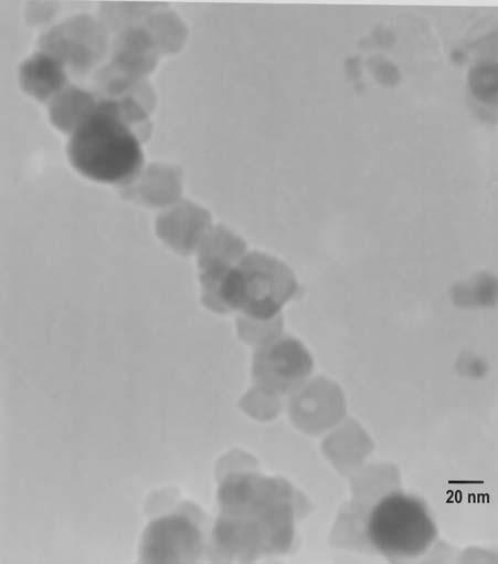
106 (a) Without Field (b) With Field Figure E.3: Samples collected at a fixed flowrate 35/450 cc/min at 20 mm height with and without Magnetic field at 45 C cylinder temperature (a) Without Field (b) With Field Figure E.4: Samples collected at a fixed flowrate 35/450 cc/min at 20 mm height with and without Magnetic field at 55 C cylinder temperature 90

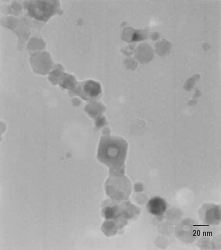
107 E.2 Samples taken at various flow rates of Fe(CO) 5 (a) Without Field (b) With Field Figure E.5: Samples collected at a fixed cylinder temperature of 35 C at 20 mm height with and without Magnetic field at a flow rate of 450cc/min CO and 25cc/min Fe(CO) 5 (a) Without Field (b) With Field Figure E.6: Samples collected at a fixed cylinder temperature of 35 C at 20 mm height with and without Magnetic field at a flow rate of 450cc/min CO and 35cc/min Fe(CO) 5 91

108 (a) Without Field (b) With Field Figure E.7: Samples collected at a fixed cylinder temperature of 35 C at 20 mm height with and without Magnetic field at a flow rate of 450cc/min CO and 45cc/min Fe(CO) 5 (a) Without Field (b) With FieldFigure Figure E.8: Samples collected at a fixed cylinder temperature of 35 C at 20 mm height with and without Magnetic field at a flow rate of 450cc/min CO and 55cc/min Fe(CO) 5 92

109 E.3 Samples taken at various heights above the burner surface (a) Without Field (b) With Field Figure E.9: Samples collected at a fixed cylinder temperature of 35 C at a flow rate of 450cc/min CO and 35cc/min Fe(CO) 5 at 12 mm height with and without Magnetic field (a) Without Field (b) With Field Figure E.10: Samples collected at a fixed cylinder temperature of 35 C at a flow rate of 450cc/min CO and 35cc/min Fe(CO) 5 at 20mm height with and without Magnetic field 93

110 (a) Without Field (b) With Field Figure E.11: Samples collected at a fixed cylinder temperature of 35 C at a flow rate of 450cc/min CO and 35cc/min Fe(CO) 5 at 30mm height with and without Magnetic field (a) Without Field (b) With Field Figure E.12: Samples collected at a fixed cylinder temperature of 35 C at a flow rate of 450cc/min CO and 35cc/min fe(co) 5 at 36mm height with and without Magnetic field 94

111 Appendix F TEM Micrographs of Samples Taken at Conditions shown in Table 9 (a) Without Field (b) With Field Figure F.1: Samples of 10nm collected at 35 C cylinder temperature, 10mm above burner surface 450cc/min CO and 20cc/min Fe(CO) 5 20 nm (a) Without Magnetic Field (b) With Magnetic Field Figure F.2: Samples of 20nm collected at 35 C cylinder temperature, 16mm above burner surface 450cc/min CO and 25cc/min Fe(CO) 5 95

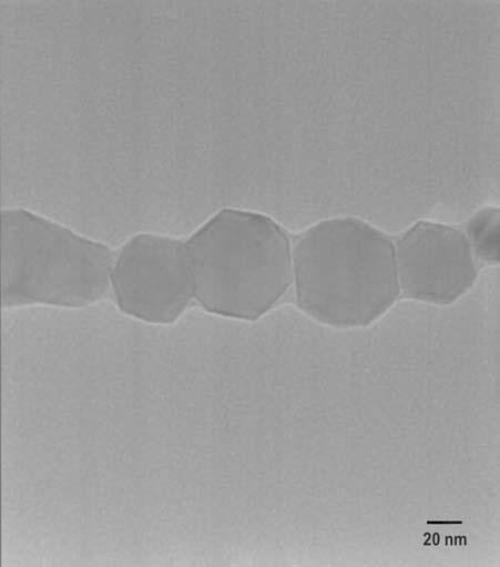
112 (a) Without Magnetic Field (b) With Magnetic Field Figure F.3: Samples of 50nm collected at 35 C cylinder temperature, 10mm above burner surface 450cc/min CO and 35cc/min Fe(CO) 5 (a) Without Magnetic Field (b) With Magnetic Field Figure F.4: Samples of 20nm collected at 45 C cylinder temperature, 10mm above burner surface 450cc/min CO and 35cc/min Fe(CO) 5 96

113 (a) Without Magnetic Field (b) With Magnet Field Figure F.5: Samples of 50nm collected at 45 C cylinder temperature, 10mm above burner surface 450cc/min CO and 45cc/min Fe(CO) 5 97

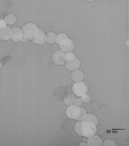
114 Appendix G TEM Micrographs of Samples at Various Cylinder Temperatures (a) Without Magnetic Field (b) With Magnetic Field Figure G.1: Samples collected at 35 C cylinder temperature, 10mm above burner surface 450cc/min CO and 55cc/min Fe(CO) 5 (a) Without Magnetic Field (b) With Magnetic Field Figure G.2: Samples collected at 45 C cylinder temperature, 10mm above burner surface 450cc/min CO and 55cc/min Fe(CO) 5 98

115 Appendix H Magnetic Recording H.1 Magnetic recording - An introduction Ferromagnetic materials are characterized by magnetization curves and Hysteresis curves. The magnetic media is often not completely saturated in magnetic recording. The external magnetic fields (H) are held below the maximum fields for saturation, and the induced magnetization (M) is correspondingly less. Thus, the induced remanent magnetization is less than the maximum M r (infinity). A more complex, but highly informative plot contains both the Hysteresis information and the remanent magnetization information. An example of such plot is illustrated for gamma ferric oxide is shown in Figure H.1. Figure H.1: Example of a hysteresis plot of a Gamma Ferric Oxide sample [32] 99

116 In the figure, M(H), aligned" is the Hysteresis curve for the particles after magnetic alignment. "M(H), random" is the Hysteresis curve for the particles with random orientation. M r (H) is the remanent magnetization curve. M ar (H) is the remanent magnetization curve for ac bias. M d (H) is the remanent magnetization after saturation in the positive field direction and successive application of a DC field in the negative direction. H.2. Recording The simplest recording system consists of a ring-shaped electromagnet with a ferrous core mounted over a ferromagnetic surface traveling at a velocity V. Since the core of the electromagnet is ferrous, the flux will preferentially travel through the core. Thus, the core is deliberately broken at an air gap. In the air gap, the flux will create a fringing field that extends some distance from the core. The signal current through the electromagnet generates a fringing magnetic field H. The fringing magnetic field H then creates a remanent magnetization on the ferromagnetic surface. Thus, the ferromagnetic surface now has become permanently magnetic. The magnetic particles in the surface act like little bar magnets themselves and create their own fringing magnetic field H above the ferromagnetic surface. Figure H.2: Simple recording system [32] 100

117 Now, assume an analog signal into the electromagnet. The analog signal will create an analog variation in H (See Figure H.3). Since the surface is moving in time, then the analog variation of the signal in time is translated into a magnetic remanent variation on the surface in space. Figure H.3: Variation of analog signal in recording [32] Thus, a very important number in magnetic recording is the spatial variation which corresponds to a signal frequency. If an incoming analog signal has a frequency f, then the characteristic wavelength of the pattern written on the magnetic media has a wavelength given by [32] It is important that the magnetic media chosen has a small enough spatial resolution to be able to support the desired frequency range at the given velocity. In many cases, the velocity may be increased in order to record the desired frequencies for magnetic media with lower spatial resolutions. 101

118 H.3. Reading The simplest reading system consists of the same head that was used to write the data on the ferromagnetic surface traveling at the same velocity V. The head now passes over the fringing magnetic fields H above the ferromagnetic surface. The voltage then induced in the electromagnet is proportional to the spatial (i.e. time, since the tape is moving) derivative of the magnetic field created by the permanent magnetization in the material [32]. Figure H.4: A simple reading system Where e = induced voltage, N = number of turns, F = magnetic surface flux and V = velocity H.4 A Prototypical tape system A typical audio tape recorder has three heads: erase, record and reproduce (See Figure H.5). During recording, the tape first moves over the erase head, where all trace of 102

119 earlier programming is removed. The erase head must also leave the head in the maximum random condition for lowest possible noise. Figure H.5: A typical tape system [32] Therefore, the erase head gap length is large to provide a strong erasing field. The erase head is also fed with an ac signal in order to minimize noise. Next the tape moves over the record head. The record head is usually fabricated with a gap size on the order of thickness of the magnetic coating. This provides a compromise between low and high frequency response. Additionally, the signal going into the record head is usually altered in two major ways from the original signal. First, an ac component is added to the signal to linearize the response. Secondly, the frequency spectrum is altered to compensate for losses that occur in the recording process for short wavelength (high frequency) signals. This compensation process (called pre-equalization) has the ultimate goal of giving the tape recorder a flat frequency response up to its maximum design frequency. Finally, the 103

120 tape moves over the reproduce head. The reproduce head is usually fabricated with a small gap in order to maximize short wavelength (high frequency) response. The inductive pick-up generates a signal which is the derivative of the flux, so the signal must be integrated. Additional equalization must be added (called post-equalization) to compensate for losses that occur in the reading process for short wavelength (high frequency) signals -- again with the intent of providing the recorder with a flat frequency response. H.5. The Media A variety of magnetic media have been used over the years. Very early recorders used ferrous wire (the "wire recorder" referred to in older books). However, most modern magnetic media use a thin layer of ferromagnetic material supported by a non-magnetic substrate. The magnetic layer can be formed of magnetic particles (such as gamma ferric oxide) in a polymer matrix. Alternatively, the layer can be a vacuum deposited metal or oxide film. The use of a thin magnetic layer permits many possible configurations for the substrate. Audio recording is largely dominated by tapes, but drums and rigid disks are also used. Digital recording at one time was completely dominated by tapes, but today has moved to flexible or rigid disks. Magnetic media are differentiated into "hard" and "soft" media. Hard media require large applied fields to become permanently magnetized. Once magnetized, large fields are required to reverse the magnetization and erase the material. Such media, with large saturation remanence and high coercivity are appropriate for such applications as computer data storage. Soft media, on the other hand, require relatively low fields to become magnetized. These low remanence, low coercivity, materials are more 104

121 H.5.1 Particulate media The ideal particulate magnetic media has isolated long ellipsoidal particles suspended either longitudinally or transversely in a matrix (See Figure H.6). Figure H.6: Particulate Magnetic media Real magnetic materials are clearly less perfect! Some photographs are reproduced below in Figure H.7 Figure H.7: Typical Magnetic materials Particulate magnetic media are most commonly used in audio tape applications. In order to insure recorder and reader compatibility, the ac bias, signal current and frequency equalization have been standardized. Thus, the coercivity, remanence and thickness are essentially set by the standardization. Improvements in performance include such things as particle alignment and morphology. Thus, in order to provide improved performance, several different standards have been established. These are summarized below in Table