EVALUATION OF FINE PARTICULATE MATTER POLLUTION SOURCES AFFECTING DALLAS, TEXAS. Joseph Puthenparampil Koruth, B.Tech.

Transcription

1 EVALUATION OF FINE PARTICULATE MATTER POLLUTION SOURCES AFFECTING DALLAS, TEXAS Joseph Puthenparampil Koruth, B.Tech. Thesis Prepared for the Degree of MASTER OF SCIENCE UNIVERSITY OF NORTH TEXAS May 2012 APPROVED: Kuruvilla John, Major Professor Srinivasan Srivilliputhur, Committee Member Aleksandra Fortier, Committee Member Costas Tsatsoulis, Dean of the College of Engineering James D. Meernik, Acting Dean of the Toulouse Graduate School

2 Puthenparampil Koruth, Joseph. Evaluation of fine particulate matter pollution sources affecting Dallas, Texas. Master of Science (Mechanical and Energy Engineering), May 2012, 92 pp., 15 tables, 36 illustrations, references, 38 titles. Dallas is the third largest growing industrialized city in the state of Texas. The prevailing air quality here is highly influenced by the industrialization and particulate matter 2.5µm (PM 2.5 ) has been found to be one of the main pollutants in this region. Exposure to PM 2.5 in elevated levels could cause respiratory problems and other health issues, some of which could be fatal. The current study dealt with the quantification and analysis of the sources of emission of PM 2.5 and an emission inventory for PM 2.5 was assessed. 24-hour average samples of PM 2.5 were collected at two monitoring sites under the Texas Commission on Environmental Quality (TCEQ) in Dallas, Dallas convention Centre (CAMS 312) and Dallas Hinton sites (CAMS 60). The data was collected from January 2003 to December 2009 and by using two positive matrix models PMF 2 and EPA PMF the PM 2.5 source were identified. 9 sources were identified from CAMS 312 of which secondary sulfate (31% by PMF2 and 26% by EPA PMF) was found to be one of the major sources. Data from CAMS 60 enabled the identification of 8 sources by PMF2 and 9 by EPA PMF. These data also confirmed secondary sulfate (35% by PMF2 and 34% by EPA PMF) as the major source. To substantiate the sources identified, conditional probability function (CPF) was used. The influence of long range transport pollutants such as biomass burns from Mexico and Central America was found to be influencing the region of study and was assessed with the help of potential source contribution function (PSCF) analysis. Weekend/weekday and seasonal analyses were useful in understanding the behavioral pattern of pollutants. Also an inter comparison of the model results were performed and EPA PMF results was found to be more robust and accurate than PMF 2 results.

3 Copyright 2012 By Joseph Puthenparampil Koruth ii

4 ACKNOWLEDGMENT First of all I would like to thank God the almighty for giving me the wisdom and knowledge and most of all health which was required to complete this research. It is an honor for me to thank Dr. Kuruvilla John, my thesis supervisor, to whom I am greatly indebted for providing me with valuable suggestions and guidance. I also thank him for providing me with research assistantship and tuition support throughout my course of this study, without which this research would have been very difficult. I would like to take this opportunity to thank Dr. Srinivasan Srivilliputhur and Dr. Aleksandra Fortier for being on my thesis committee and providing me with their valuable advice and suggestions. Last but not the least, I would like to thank my friends and my family for encouraging me and supporting me. iii

5 TABLE OF CONTENTS Page ACKNOWLEDGMENT... iii LIST OF TABLES... vi LIST OF FIGURES... vii CHAPTER 1 INTRODUCTION Study Area Goals and Objectives... 3 CHAPTER 2 LITERATURE REVIEW... 5 CHAPTER 3 DATA AND METHODOLOGY Data Collection Methodology Statistical Analysis for Raw Data PMF 2 Model EPA PMF 3.0 Model Conditional Probability Function (CPF) Potential Source Contribution Function Analysis (PSCF) CHAPTER 4 RESULTS AND DISCUSSION Raw Data Time Series Analysis Comparison of Various PM 2.5 Monitoring Data Source Apportionment Analysis Using PMF Species Selection Factor Determination and Identification iv

6 4.3.3 Source Profile Identification Source Contributions Conditional Probability Function (CPF) Source Apportionment Analysis Using EPA PMF Species Selection Source Profile Identification and Contribution Conditional Probability Function (CPF) Potential Source Contribution Factor (PSCF) Analysis CHAPTER 5 INTER-COMPARISON OF PMF 2 AND EPA PMF 3.0 MODEL RESULTS CHAPTER 6 CONCLUSION AND RECOMMENDATIONS APPENDIX A GRAPHS AND TABLES USED IN PMF 2 ANALYSIS APPENDIX B GRAPHS AND TABLES USED IN EPA PMF 3.0 ANALYSIS APPENDIX C GRAPHS USED FOR INTER COMPARISON OF THE MODEL RESULTS. 87 REFERENCES v

7 LIST OF TABLES Table 1: Details of TCEQ CAMS 312 and CAMS Table 2 : List of days with high PM 2.5 concentration for CAMS 312 and CAMS Table 3: Species distribution in traffic source profile at CAMS 312 and CAMS Table 4 : Species distribution for industrial source profile at CAMS 312 and CAMS Table 5 : Species distribution for aged sea salt profile of CAMS 312 and CAMS Table 6 : Species distribution for biomass profile of CAMS 312 and CAMS Table 7: Species distribution for roadside crustal profile of CAMS 312 and CAMS Table 8: Species distribution for secondary sulfate II profile of CAMS 312 and CAMS Table 9: Species distribution for crustal profile of CAMS 312 and CAMS Table 10: Species distribution for secondary nitrate profile of CAMS 312 and CAMS Table 11: Species distribution for secondary sulfate profile of CAMS 312 and CAMS Table 12: Species distribution for secondary sulfate II comingled with industrial profile of CAMS 312 and CAMS Table 13: Comparison of source profiles identified from CAMS 312 by PMF 2 and EPA PMF Table 14: Comparison of source profiles identified from CAMS 60 by PMF 2 and EPA PMF Table 15: Variation in concentration of the sources in hot and cold seasons Page vi

8 LIST OF FIGURES Figure 1: Location of the TCEQ CAMS in Dallas County... 3 Figure 2: Time series analysis ( ) for CAMS 312 and CAMS 60 (a) yearly (b) seasonal and (c) monthly Figure 3: Time series analysis of PM 2.5 for CAMS 312 and CAMS60 for '03-' Figure 4: 24 hours back trajectories on days with high PM 2.5 concentrations at (a) CAMS 312 and (b) CAMS Figure 5: PM 2.5 speciated data versus PM 2.5 TEOM for CAMS 312 and CAMS Figure 6 : Fpeak analysis for 9 factors of CAMS Figure 7 : Fpeak analysis for 8 factors of CAMS Figure 8: Source contributions observed at CAMS 312 for Figure 9 : Source contribution observed at CAMS 60 for Figure 10: CPF plots for traffic profile for CAMS 312 and CAMS Figure 11: CPF plots for aged sea salt profile for CAMS 312 and CAMS Figure 12: CPF plots for biomass profile for CAMS 312 and CAMS Figure 13: CPF plots for crustal profile for CAMS 312 and CAMS Figure 14: CPF plots for secondary sulfate profile for CAMS 312 and CAMS Figure 15: CPF plots for secondary nitrate profile for CAMS 312 and CAMS Figure 16: CPF plots for industrial source profile for CAMS 312 and CAMS Figure 17: CPF plots for secondary sulfate II comingled with industrial source for CAMS Figure 18: CPF plot for secondary sulfate II for CAMS Figure 19 : Residual analysis output of sulfur from EPA PMF 3.0 GUI for CAMS Figure 20 : O/P scatter plot for sulfur from EPA PMF 3.0 of CAMS Figure 21 : O/P time series analysis for sulfur of CAMS Figure 22 : Source contribution and percentages of each factors of CAMS Page vii

9 Figure 23 : Source contribution and percentages of each factors of CAMS Figure 24: CPF plot for CAMS 60 for secondary sulfate II and road side crustal Figure 25 : PSCF analysis of biomass burns on Dallas using CAMS Figure 26 : PSCF analysis of biomass burns on Dallas using CAMS Figure 27: PSCF analysis of secondary sulfates on Dallas using CAMS Figure 28: PSCF analysis of secondary sulfates on Dallas using CAMS Figure 29 : PSCF plots for crustal dust showing that the dust is transported from Africa for CAMS Figure 30 : PSCF plots for crustal dust showing that the dust is transported from Africa for CAMS Figure 31 : Comparative illustration of source identified from CAMS 312 using PMF 2 and EPA PMF Figure 32: Comparative illustration of source identified from CAMS 60 using PMF 2 and EPA PMF Figure 33: Weekend-weekday analysis at CAMS 312 using PMF2 and EPA PMF Figure 34 : Weekend-weekday analysis for common sources at CAMS 60 using PMF2 and EPA PMF Figure 35: Seasonal analysis for CAMS 312 inter-comparison of results for sources where (a) winter (b) spring (c) summer (d) fall Figure 36: Seasonal analysis for CAMS 60 inter-comparison of results for common sources where (a) winter (b) spring (c) summer (d) fall viii

10 CHAPTER 1 INTRODUCTION Particulate matter pollution is an area of major interest in the urban regions on this planet. Ambient particulate matter is increasingly becoming a concern around the globe due to its negative effects on human beings. Major health hazards identified are respiratory problems and health effects leading to premature mortality. This is mostly due to the increased exposure to fine particulate matter less than 2.5μm classified as PM 2.5, which includes organic carbon, elemental carbon and oxygenated hydrocarbons (Metzger et al., 2004). Studies on the health effects of particulate matters that have been conducted based on seasonal and sub seasonal results showed that death rates are high in winter than in summer and as a result of short-term episodes (Burnett et al.,1998). In addition, PM 2.5 contributes to visibility impairment and acid deposition (Watson, 2002). Several of these studies on health hazards and environmental impact resulted in the United States Environmental Protection Agency (US-EPA) in the year 1997 to declare fine particulate matter as one of the criteria air pollutant and introduced new standards for PM 2.5 (Federal Register, 1997). It is important to understand which emission sources contribute to the elevated daily PM 2.5 levels and what control strategies must be applied to keep it within the standard limits. The key aspect of air quality control lies in identifying the correct sources of the pollutant. Each state in the US has a state implementation plan (SIP) and regulatory bodies that impose laws and regulatory actions to meet the national ambient air quality standards (NAAQS). In order for them to execute regulatory actions it is vital to identify the proper source profiles. Therefore, an increased emphasis on the particulate matter analysis is required. 1

11 The source receptor model has been proven to be an important tool in the identification of particulate sources by calculating the concentration of pollutants at the receptor site (Hopke P. K, 1991). In this study, a highly speciated ambient air quality data based on a 24-hour sampling was collected at two receptor sites from January 2003 through December 2009 in Dallas, Texas. Dallas is the third largest city in the state of Texas (ALMANAC Facts Profile, 2011) with a population of approximately 1.2 million as of 2010 (Census Bureau, 2010). It is a rapidly growing urban area with increasing air quality concerns. To date, there have been no major PM 2.5 source apportionment studies conducted in Dallas. The aim of the current study was to identify and quantify the sources of PM pollution and to compare the results of two source apportionment models. 1.1 Study Area Air quality data from two ambient monitoring sites in Dallas are used in this study. The Texas commission on environmental quality (TCEQ) operates and maintains continuous ambient monitoring stations (CAMS) that measure PM 2.5, PM 10, NO X, SO 2, O 3, CO and other air quality parameters. CAMS 312 and CAMS 60 were located at an approximate distance of 6 miles apart, at 32º 46' 27'' North, -96º 47' 52'' West and 32º 49' 12'' North, -96º 51' 36'' West respectively in Dallas county. The locations of the study areas and the TCEQ CAMS sites are shown in Figure 1. Table 1 provides further details of these sites. 2

12 CAMS 60 CAMS 312 Figure 1: Location of the TCEQ CAMS in Dallas County Table 1: Details of TCEQ CAMS 312 and CAMS 60 CAMS No Region Site Location EPA SITE County ID 0312 Dallas 717 south Akard st, Dallas Dallas, TX 060 Dallas 1415 Hinton Street, Dallas, TX Dallas There are number of other TCEQ sites monitoring several air quality parameters but since this study was focused on PM 2.5 emission, only these two sites were considered. Both sites 24- hour averaged PM 2.5 concentration data collected every 3 rd day. 1.2 Goals and Objectives The primary goal of this study was to identify and quantify the sources for PM 2.5 emission in Dallas, Texas. Data from CAMS 312 and CAMS60 was analyzed to identify the sources of PM 2.5 using source apportionment techniques such as PMF2 and EPA PMF 3.0. The results are compared to understand the ability of the two models to perform source apportionment and also 3

13 to ensure the accuracy of the results. In prior studies over similar urban airsheds, industrial sources and vehicular emissions were identified having a huge role affecting the air quality in those areas. It was hypothesized that similar sources would have a major role in air quality of Dallas. In order to substantiate this hypothesis, source receptor analysis was performed and source contributions were identified with the help of PMF2 and EPA PMF 3.0. Following are the major objectives of this study: Perform time series analysis to evaluate the PM 2.5 concentration trends Conduct data analysis to understand the robustness of the collected data Identify the source profiles and corresponding source contribution for each site Understand the effect of meteorological factors on the distribution of PM 2.5 by using condition probability function (CPF) Evaluate two source apportionment models (PMF2 vs. EPA PMF) Conduct potential source contribution function analysis (PSCF) to identify the upwind source region affecting the air quality in the study area Chapter 2 describes recent studies conducted using source apportionment models. Chapter 3 focuses on the methodology. Results and discussions are described in Chapter 4 where detailed analysis results of PMF2 and EPA PMF are included. Inter comparison of the model results are summarized in Chapter 5 and finally Chapter 6 provides conclusions from this study and recommendations for future studies. Appendices A and B list the emission inventory and outputs from PMF2 and EPA PMF 3.0, respectively. Additional graphs and tables from inter comparison of models are given in Appendix C. 4

14 CHAPTER 2 LITERATURE REVIEW Pollution in the atmosphere, a subject of major concern, can be attributed to many chemical species such as ozone, volatile organic carbon (VOCs), carbon monoxide, particulate matter etc. Out of this particulate matter smaller than 2.5µm is responsible for serious health problems and major environmental issues. The serious effects of particulate matter pollution and its strong relation to mortality was the subject of the studies conducted by Dockery et al. (1993). By studying data related to mortality due to cardiovascular and respiratory diseases, the authors were able to find a strong effect of air pollution on the death rates. This study had an important role in the EPA s decision to regulate PM 2.5 (EPA, 1996). Owing to the importance of this topic, Klemm et al. (2000) reconstructed and replicated the analysis and produced results, which matched the original findings of Dockery et al. (1993). There are several source apportionment models in use today viz., chemical mass balance (CMB) receptor model, positive matrix factorization (PMF), principal component analysis/absolute principal component scores (PCA/APCS) and UNMIX. Each of the models has its pros and cons; for example, CMB is time consuming and has a difficult methodology when it comes to measurement of source profiles. The source profiles are limited to certain urban areas of United States and Europe (Song et al., 2006). A study conducted by Miller et al. (2002) compared PMF, CMB, PCA/APCS and UNMIX. This study concluded that PMF was the able to extract the major sources and appeared to be the best, and that UNMIX responded well to variablity in data. However, none of these models could identify sources which contributed to less than 5% of the total measured concentration. Understanding the higher accuracy of PMF as compared to other models, in discerning sources, PMF was used for source apportionment in the 5

15 current study. Also for the very same reason PMF was widely used by resarchers in earlier similar studies. Identifying the source is the most difficult part in any source apportionment model. Researchers in the past have identified the composition of many source profiles such as crustal dust, industrial dust, traffic, aged sea salt, biomass etc. (Lee et al., 2008; Karnae and John 2011). Having such information on source profile eases the approach towards a definitive agreement of a particular source. The source profiles such as traffic, industrial dust, roadside crustal dust etc. are mostly common in major urban air sheds in the United States (Lee et al., 2008), Europe (Laupsa et al., 2009) and Australia (Chan et al., 2011). PMF is a multivariant receptor model which is based on the least square technique (Paatero, 1997).Whereas multilinear engine, another model used to solve various multilinear problems (Paatero, 1999), is more flexible as it incorporates rotational functions and is accurate in identifying the source profiles. Both these techniques are widely used for source apportionment but have the drawback of not being user friendly as these are DOS based programs. For this reason EPA developed a more user friendly tool, EPA PMF V1.1. Recent studies found that there were differences in the results obtained using EPA PMF V1.1 and PMF 2 on sites in Chicago while identifying the minor sources (Kim and Hopke, 2007). This was because the EPA PMF V1.1 did not provide any rotational functions as implemented in PMF 2 (Hwang and Hopke, 2011). For this very reason, US EPA upgraded EPA V1.1 to EPA PMF 3.0 which uses multilinear engine ME-2 as its skeleton (EPA PMF 3.0, 2008). Ramadan (2003) showed that there are many uncertainties in PMF2 and that there is better source identification by ME-2. This leads to the hypothesis that EPA PMF 3.0, which is derived from ME-2, would provide better source apportionment results than PMF 2. 6

16 As mentioned earlier there have been a number of research studies conducted using PMF 2 in many places across the globe. However very few studies have done a comparative analysis of PMF2 and EPA PMF 3.0 (Chan et al., 2011; Hwang and Hopke 2011). Hence the current study also focuses on comparing the two model results. The location of the pollutant source is identified by a conditional probability function (CPF) which uses wind speed and wind direction data to complete this task. There are several long range transport pollutants affecting the study region which are identified using a procedure called potential source contribution function (PSCF) analysis. Karnae and John (2011) found that the biomass burns in Central America region and secondary sulfates from Ohio River Valley affect the urban air shed of Corpus Christi, Texas. Dallas has complex and multiple emission sources and is impacted by seasonally varying wind patterns. Studies by Xie and Berkowitz (2006) conducted in similar regions were supported by CPF and PSCF analyses in identifying the sources; therefore it would be justifiable to use CPF and PSCF in the current study. 7

17 CHAPTER 3 DATA AND METHODOLOGY The data from both the Texas Commission on Environmental Quality (TCEQ) monitoring sites continuous ambient monitoring stations (CAMS) 312 and CAMS 60 were collected and were analyzed using PMF models. Further, in this section PM 2.5 data acquisition, source apportionment analysis, conditional probability function (CPF) and potential source contribution function analysis (PSCF) are discussed. 3.1 Data Collection As previously mentioned, two sites in Dallas, Texas were selected for data collection related to the current study. The 24-hour averaged PM 2.5 data from TCEQ CAMS 312 and CAMS 60 are collected every 3 days using a Whatman Teflon filter of 47 mm diameter with a pore size of 2µm and quartz pre weighted filters. These filters are shipped to Research Triangle Institute (RTI) in North Carolina (Karnae and John, 2011) for analysis. RTI takes this sample and does a gravimetric and chemical analysis using energy dispersive X-ray fluorescence. Water soluble ions are analyzed using chromatograph (EMEP/CCC, 1996) and the carbon species are analyzed using thermo-optical transmittance (M.E Brich, 1996). The results of this analysis are archived in TCEQ repository. The data from January 2003 to December 2009 was requested and acquired from TCEQ was used in this study. 3.2 Methodology The robustness of the data is confirmed by comparing with the 24-hour averaged concentration obtained from a tapered element oscillating microbalance (TEOM) with the 8

18 speciated filter mass data. Two different source apportionment models which follow the principle of positive matrix factorization (PMF) are used in this study. To substantiate the source profiles results, conditional probability function (CPF) and potential source contribution function (PSCF) are also used. The methodologies employed in this study are explained in the following section Statistical Analysis for Raw Data Raw data collected from TCEQ sites are compared with 24-hour average TEOM data from a nearby site to understand the robustness of the collected data. Statistical analysis of plotting the two data sets in a scatter plot and performing linear fit helps in examining the data. If the regression coefficient is poor the data needs to be verified and discarded as needed. The TEOM data values would be lesser than the speciated data as there is a possibility of the volatile organic compounds and other semi-volatile elements escaping during the measurement process. Whereas in speciated data measurement these elements are captured on the Teflon filters and considered during the measurement. When the plot is divided into two sections the majority of the data points should be towards the speciated data axis, hence proving that speciated data being used are robust and also includes the volatile compounds. The raw data needs to be analyzed for yearly and seasonal trends to understand the variation of PM over the years and also the behavioral pattern during seasonal change. Also high PM 2.5 days should identified and 24-hour backward trajectory analysis needs to be performed to understand how the transport of pollutant has occurred. 9

19 3.2.2 PMF 2 Model Basic Theory Positive matrix factorization (PMF) developed by Paatero (1997) does factor analysis using equation 1 and this equation serves as the basis of the analysis. (1) where x represents the mass concentration matrix of order two by two, is the mass concentration of the j th species and i th sample. g represents the matrix of source contributions, is the PM 2.5 concentration from the k th factor in the i th sample. f is the matrix of source profile, is mass concentration of the j th species in the k th factor and is the residual associated with the concentration of the j th species in the i th sample. The objective of PMF is to minimize of the sum of residual equation (EPA PMF 3.0, 2008) which is given as ( ) [ ] [ ] where (2) is data uncertainty for the j th species in the i th sample. PMF2 varies the matrix G and F simultaneously in each iterative step (Hopke, 2000). There are cases where a species is not measured as its concentration value goes below the method detection limit (MDL), also there would be cases where there are no values measured. Hence MDL for each species is used to determine the accuracy in the measurement of the concentration of the species. 10

20 Species Selection There would be species which are observed but may not be consistent and may be an insignificant portion in mass concentration of source samples; also, they are found to have relatively less lifetime in the ambient air (Liu, Shao, Zhang, Fu, and Lu, 2005). To identify which species needs to be included in the source apportionment analysis Hopke has suggested the method of using signal to noise ratio (S/N) (Paatero and Hopke, 2003). Equation (3) used to calculate S/N for PMF 2.0. S/N = { } (3) where is the concentration amount of the j th species collected at i th interval of time, which is greater than the MDL. is the mean of the MDL of j th species and is the count of number of values less than the MDL. With the S/N ratio is used for species selection. Species with S/N ratio less than 0.2 were classified as bad species and they are eliminated from further analysis. Species with S/N ratio between 0.2 and 2 are considered as weak and finally for the species that has S/N ratio above 2 is considered as Strong (Paatero and Hopke, 2003) Data Preprocessing Data preprocessing is one of the primary steps of source apportionment analysis. Once this step is completed then the data has to be properly arranged for further analysis. There might be days for which PM 2.5 species data would be missing; those days are removed. There are dates where all species are missing and these should be eliminated from the data set, as well. 11

21 Estimation of Weights Hopke (2000) has mentioned how to create concentration and uncertainty file. In order to minimize the error estimate the following methods were applied. If the >MDL ij = for the determined value for data below (4) for missing values, where is the mean Determination of the Number of Factors PMF requires the user to choose number of factors beforehand. This is one of the primary steps that need to be followed. A brief idea of sources in the region under analysis would be an added benefit in reducing the time. Vector space rotation is controlled using the Fpeak value, which is yet another important parameter in PMF. It is very hard to find a unique solution even if there is a global minimum in the least fitting process (Hopke, 2000). Fpeak value ranges from -1 to 1 with zero as the central value. Keeping Fpeak at zero can produce a central solution whereas varying the values can provide sharp peak values. Hence Fpeak values are varied in order to reduce the rotational ambiguity and to get an optimal solution (Kim and Hopke, 2008). Final PMF solution is obtained by series of iteration. 12

22 3.2.3 EPA PMF 3.0 Model EPA PMF 3.0 has similar theory and equations as PMF2. When compared with PMF2, EPA PMF 3.0 has greater accuracy and lesser uncertainty as it uses multilinear engine (ME) as a skeleton for EPA PMF 3.0 as mentioned in before section. There are few differences in how the species selections are performed and determination of Q value which are mentioned in the following section Species Selection The additional analyses performed by EPA PMF 3.0 for species selection are explained below Species Selection In EPA PMF 3.0 there is a significant difference in calculation of signal to noise ratio. EPA PMF 3.0 uses equation (4) to calculate S/N (EPA PMF 3.0, 2008). S/N = ( ) (5) The classification of weak, strong and bad species are as presented by Paatero and Hopke (2003) (EPA PMF 3.0, 2008). Bad species are eliminated from further analysis. In this model S/N is not the ultimate method of species selection in EPA PMF Residual Analysis The histogram showing the percent of all scaled residuals can be located in the graphical user interface (GUI). These plots are helpful in understanding the fit of each species. If the species has a good distribution it is considered to be strong and ones with a wider distribution 13

23 and poor fit are classified as weak whereas the species which has poor distribution are classified as bad. Further analysis between runs can be performed using the following equation ( ) (6) where r is scaled residual, i is the species sample, j is variable and k and l are separate runs. The d values for each species are summed up for each runs. This expressed as a matrix of base run pair and is examined for large variation which proves the different runs are different solutions and not an output of mere rotation (EPA PMF 3.0, 2008) Observed/Predicted (O/P) Scatter Plot The O/P scatter plot in the GUI helps identify the robustness of the model. The species observed and predicted concentrations are shows as graphical image in the GUI. The species with poor correlation coefficient values needs to be classified as weak or bad (EPA PMF 3.0, 2008) Observed/ Predicted (O/P) Time Series The O/P times series in the GUI displays is having the same data of O/P scatter plot but displayed as time series. If the predicted value is not fitting with the observed value then the species should be down weighted or eliminated from further analysis (EPA PMF 3.0, 2008) Determination of Factors Number of factors is determined by the user s knowledge on the region and the potential sources surrounding the receptor site. The fit of the model would finally determine if the selected 14

24 number of factors are appropriate or not, bootstrap runs are performed to understand this. The variability of the factors are given by as the mean of 5 th, 25 th, 75 th and 95 th percentile of median of the Q (robust) values this helps in determining the number of factors. Also EPA PMF 3.0 provides a facility to perform different iterations in same run. Hence enabling the user to evaluate different runs and determine the number of factors Conditional Probability Function (CPF) Identifying the sources would not be enough to quantify the emissions. The physical location of each source groups must be identified to substantiate the results. For this conditional probability function (CPF) is used. The results of the PMF analysis and surface wind direction are used to calculate CPF. It may be defined as CPFΔθ = where is number of times the source contribution estimate of PMF exceeds the 75 th percentile of all the concentration of a give factor from a given site and is the total number of sample from same wind sector (Kim and Hopke, 2004). A polar coordinate plot is made based on the magnitude of CPF and angle of the associated wind direction. This point out the location from where the fractions of samples are coming from. There are some assumptions associated with CPF analysis that the air parcel is arriving at a receptor site in a straight line path from the source. This assumption stands true only for sources, which are in proximity to the receptor, but in general, this is not true (Xie and Berkowitz, 2006). CPF is an approximate method but with the understanding of the region it can aid in identifying the sources. 15

25 3.2.5 Potential Source Contribution Function Analysis (PSCF) Potential source contribution function analysis (PSCF) has been used widely to identify the regional sources that increase the level of pollutant concentration. PSCF is calculated with probability of concentration in each points and are calculated using the following equation where is the number of points having concentration above a threshold and represents the number of endpoints of back trajectories that pass through each grid cell (Karnae and John, 2011). And the backward trajectories required for the analysis is generated using a model developed by National oceanic and atmospheric administration (NOAA), which is called hybrid single particle Lagrangian integrated trajectory (HYSPLIT4) model. The concentration level of the pollutant in each of the endpoint is calculated. Using the geographical information system (GIS) a spatial grid of required resolution is generated and a threshold of 75 th percentile is set for the apportioned mass of each source. There could be uncertainties in grid cells with low number of trajectory endpoints caused by higher PSCF values, this needs to be reduced and is done by multiplying the PSCF values with an arbitrary weight function W (Karnae and John, 2011). W the weight function is expressed as the following ( ) { 16

26 CHAPTER 4 RESULTS AND DISCUSSION A detailed analysis was performed on the air quality data obtained from two TCEQ sites (CAMS 312 and CAMS 60) using two source apportionment models (EPA PMF 3.0 and PMF2). The data from these two sites were analyzed and a time series analysis was performed for both the sites. In addition, a 24-hour back trajectory analysis was performed for days with high PM 2.5 concentration and the corresponding results are explained along with the results from the source apportionment models involved in this study are explained in this chapter. 4.1 Raw Data Time Series Analysis The time series analysis for the raw speciated data was performed for two sites in Dallas, CAMS 312 and CAMS 60, using the averages of the total PM 2.5 measured in these sites. Averages are used because both the sites have different observation dates and number of observations. The time series analysis was performed based on annual, seasonal and monthly data as shown in figure 2. (1)Total PM 2.5 Vs Year for the CAMS 312 and CAMS 60 Average PM 2.5,µgm Years CAMS 312 CAMS 60 (a) 17

27 (2) Total PM 2.5 Vs Seasons for CAMS 312 and CAMS 60, '03-'09 Average PM 2.5,µgm Spring Summer Fall Winter CAMS 312 CAMS 60 Seasons (b) Average PM 2.5,µgm (3) Total PM 2.5 Vs Months for CAMS 312 and CAMS 60, '03-'09 CAMS312 CAMS60 Months (c) Figure 2: Time series analysis ( ) for CAMS 312 and CAMS 60 (a) yearly (b) seasonal and (c) monthly From figure 2(a), it was observed that CAMS 312 had higher PM 2.5 concentration during all years. A careful analysis of the trends revealed a decrease of 3.5 ppb (25%) for CAMS 312 during the study period, while a 3 ppb (24%) decrease was noted at CAMS 60 for the same study period. Year 2005 had the highest PM 2.5 concentration observed for the analyzed years. Figure 2(2) shows the seasonal variations of PM 2.5 concentrations. Summers showed the highest average concentration of 14 ppb and the lowest concentrations were observed during the winters with an 18

28 average concentration of 11 ppb. This is further explained in figure 2(c), which shows the average PM 2.5 concentration distributed over the months. PM 2.5 concentration was observed to increase during to the warm summer months of May through September and showed lower levels during the other months. The time series analysis for the hourly PM 2.5 concentration was completed and is shown in figure 3. It was noted that there were fewer days with PM 2.5 concentrations above 30µgm -3. CAMS 312 recorded 10 high PM 2.5 days for the entire time period and CAMS 60 recorded 5 high PM 2.5 days, and these are shown in table 2. Figures 3(a) and (b) shows the time series plot of measured PM 2.5 for CAMS 312 and CAMS 60, respectively. The points above the red dotted line indicate high PM 2.5 concentration days. Table 2 : List of days with high PM 2.5 concentration for CAMS 312 and CAMS60 CAMS 60 CAMS 312 Days Concentration µgm - 3 Days Concentration µgm - 01/27/ /27/ /06/ /6/ /09/ /9/ /21/ /21/ /07/ /20/ /27/ /7/ /19/ /8/ /15/

29 (a) (b) Figure 3: Time series analysis of PM 2.5 for CAMS 312 and CAMS60 for '03-'09 A 24-hours backward trajectory analysis using NOAA s HYSPLIT4 was performed on the identified high PM 2.5 days. From figures 4 (a) and (b) it was found that some of the air 20

30 parcels traveled from outside the state and some even over the Gulf of Mexico. To understand further about these long range transport of pollutants, a detailed PSCF analysis was conducted using back trajectory data. (a) Figure 4: 24 hours back trajectories on days with high PM 2.5 concentrations at (a) CAMS 312 and (b) CAMS 60 (b) 4.2 Comparison of Various PM 2.5 Monitoring Data TCEQ employs the tapered element oscillating microbalance (TEOM) to measure PM 2.5 mass concentrations on a continuous basis. Data reported from TEOMs are typically reported as hourly averaged concentration values. PM 2.5 mass concentrations collected using the TEOM at CAMS 60 was used for a correlational analysis with mass concentration data from the filter based speciated mass data collected at CAMS 60 and CAMS 312. Hourly TEOM data from January 2003 to December 2009 was collected and the 24-hour averages were calculated. Since speciated data was not available for every day the TEOM data was arranged to match the days 21

31 for which the speciated data was present. Figure 5(a) shows the correlation between TEOM and speciated data for CAMS 312. (a) (b) Figure 5: PM 2.5 speciated data versus PM 2.5 TEOM for CAMS 312 and CAMS 60 The correlation coefficient was noted to be 0.75 and from the figure it can be identified that most of the data points were over the 45 o line (marked in blue) this possibly highlights the mass loss due to volatile compounds being vaporized during TEOM measurement. whereas the speciated data includes all the species. Figure 5(b) shows a similar analysis for CAMS 60 where the correlation coefficient was noted to be The colocated site (CAMS 60) showed a higher corelation than CAMS 312. The results noted from this analysis proved that the data acquired from the two speciated sites was reasonably robust and that this can be further analyzed and used for source apportionment analysis. 4.3 Source Apportionment Analysis Using PMF 2 PMF 2 was applied to concentration data obtained from both the sites to perform a detailed source apportionment analysis. The steps undertaken and the corresponding results are mentioned in the subsequent sections. 22

32 4.3.1 Species Selection Equation (3) serves as the basis for species selection. As mentioned in section , the S/N ratio determines the classification of the species and based on this the species were either included or excluded. A total of 62 species were collected from CAMS 312, after using the S/N ratio, 25 species were identified to be strong species, while 10 species were identified to be weak, and the rest (27 species) were considered to be bad or poor species and the bad species were eliminated from further analysis. At CAMS 60, the total number of collected species was 63 and based on the S/N ratios 28 species were identified as strong, 13 as weak and these were retained for the analysis, while the remainder (22 species) were eliminated. Appendix A contains the complete list of species classified by their respective strengths Factor Determination and Identification Factor identification is an important part of the PMF analysis. The theoretical Q value was compared with the actual Q value to confirm fewer errors. Furthermore, an Fpeak analysis was performed on the modeled results; where the main objective was to find a flat bottom curve in the plot of Q versus Fpeak. Figures 6 and 7 highlight the 9 factors plot for CAMS 312 and the 8 factors plot for CAMS 60. This illustrates that the 9 factor and 8 factor plots showed a flat bottom and thus these were considered for further analysis. The other Fpeak analyses are included in Appendix A. 23

33 Figure 6 : Fpeak analysis for 9 factors of CAMS 312 Figure 7 : Fpeak analysis for 8 factors of CAMS Source Profile Identification Nine sources were identified for CAMS 312, based on the composition of the different chemical species in it. The source profiles identified were: traffic, industrial, aged sea salt, biomass, roadside crustal, secondary sulfate II, secondary sulfate, crustal and secondary nitrate. Whereas at CAMS 60 8 factors were identified and the corresponding source profiles identified 24

34 included: secondary sulfate, aged sea salt, a co-mingled of secondary sulfate II with industrial sources, crustal, traffic, industrial, biomass and secondary nitrate. (a) Traffic Source Profile This source is characterized by organic carbon, elemental carbon, OC1, OC2, OC3, OC4. The table 3 compares the percentage distribution of each element observed at both the sites. Table 3: Species distribution in traffic source profile at CAMS 312 and CAMS 60 Elements CAMS 312 CAMS 60 OC 91.50% 75.20% EC 18.10% 6.70% OC % 17.40% OC % 16.60% OC % 13.20% OC % 18.30% These species are the byproducts of hydrocarbon combustion. Usually these species are emitted from internal combustion engines in vehicles. Hence this source was identified as traffic/vehicular exhaust (Laupsa et.al, 2009). From table 3 we can conclude that CAMS 312 showed a slightly higher influence of traffic and the reason for this was due to the fact that the site is located adjacent to major highways and traffic arteries. (b) Industrial Source profile This source is composed of zinc, iron, lead, manganese and trace amounts of arsenic and yttrium, and is considered as a typical industrial source signature (Lee et al., 2008). Table 4 illustrates the percentage distribution of species observed at both sites. 25

35 Table 4 : Species distribution for industrial source profile at CAMS 312 and CAMS 60 Elements CAMS 312 CAMS 60 Fe 6.00% 6.50% Zn 0.65% 0.60% Pb 0.12% 0.11% Mn 0.15% 0.17% Ca 2.00% 6.30% Cu 0.33% 0.28% CAMS 312 and CAMS 60 are surrounded by small scale industries such as grinding, recycling, industrial equipment manufacturers and electronic component manufacturing industries. These industries emit the above mentioned elements. From this composition along with the study of the area, it can be concluded that this factor was primarily an industrial source. (c) Aged Sea Salt Source Profile Aged sea salt is often identified with the increased presence of sulfate ion and ammonium ion along with sodium ion as chloride ion is easily displaced by the former ions. Sources with this profile can be classified as aged sea salt (Kim and Hopke, 2008). Table 5 : Species distribution for aged sea salt profile of CAMS 312 and CAMS 60 Elements CAMS 312 CAMS 60 Na 16.34% 12.83% Na % 14.52% Cl 0.49% 0.73% Key species in this factor profile include Na, Na +, Cl - and some trace amounts of other species. This factor was thus classified as aged sea salt. The mass concentration of aged sea salt 26

36 noted at CAMS 312 was 4.7% and it was 5.4% for CAMS 60. These levels were considered as reasonable due to the fact the Dallas is an inland urban area. (d) Biomass Source Profile Biomass burns (Oguleia et al., 2006) also known as wood burning (Liua et al., 2005) or vegetative burns (Wu et al., 2007) is often identified by the presence of potassium and organic carbon in the measured PM 2.5 concentration as these key species are released to atmosphere during the combustion process associated with the burning of biomass. Table 6 : Species distribution for biomass profile of CAMS 312 and CAMS 60 Elements CAMS 312 CAMS 60 K 7.60% 5.17% K+ 7.22% 8.45% OC 24.84% 28.62% Table 6 shows the distribution of potassium and organic carbon in this factor and the species distribution was noted to be similar to the findings from other research studies (Oguleia et al., 2006; Liua et al., 2005; Wu et al., 2007). (e) Roadside Crustal Profile Road side crustal profile was identified only at CAMS 312. The location of the site is in downtown Dallas and is surrounded by roads and interstate highways. Usually road side crustal or soil and road dust (Laupsa et al., 2009) is characterized by calcium, iron, silicon, zinc and organic carbon. The composition of species in Table 7 is similar to the road side crustal source identified in Laupsa et al (2009). 27

37 Table 7: Species distribution for roadside crustal profile of CAMS 312 and CAMS 60 Elements CAMS 312 CAMS 60 Ca 20.02% - Si 2.41% - Fe 3.83% - OC 22.02% - OC2 11.9% - (f) Secondary Sulfate II Profile Table 8 shows that this profile is composed of 20.75% of S and % of OC. From earlier studies, secondary sulfate II profiles have strong composition of sulfur and organic carbons (Kim and Hopke, 2006). Since this profile was characterized by high concentrations of sulfur and organic carbon, this was identified as secondary sulfate II. Table 8: Species distribution for secondary sulfate II profile of CAMS 312 and CAMS 60 Elements CAMS 312 CAMS 60 S 20.75% - S % - NH 18.80% - OC 38.14% - (g) Crustal Profile Crustal profile is often characterized by the presence of high concentrations of silicon and aluminum. At both CAMS 312 and CAMS 60, we have identified the crustal profile as an important component affecting the measured air quality. Table 9 shows the distribution of Si, Ti, and Al at CAMS 312 and CAMS

38 Table 9: Species distribution for crustal profile of CAMS 312 and CAMS 60 Elements CAMS 312 CAMS 60 Si 19.41% 11.07% Ti 0.73% 3.33% Al 9.19% 3.39% Sources having similar composition in other studies were classified as crustal dust (Kocak, 2009) and also as dust from construction (Qin, Kim, and Hopke, 2006). (h) Secondary Nitrate Profile Secondary nitrate is primarily associated with anthropogenic emissions from industrial activities and also due to some natural sources. There was a high percentage of NO , and NH 4 noted at CAMS 312 and CAMS 60 as shown in table 10. An earlier study conducted in Corpus Christi (Karnae and John, 2011) and also in Beijing (Song, et al., 2007), factors with similar profiles were identified as secondary nitrate. Table 10: Species distribution for secondary nitrate profile of CAMS 312 and CAMS 60 Elements CAMS 312 CAMS 60 NO % 54.21% Total Nitrate % NH % 17.36% (i) Secondary Sulfate Profile Secondary sulfates are usually associated with the long range transport of photochemically aged air mass containing smog particles and this is typically highlighted by the 29

39 presence of significant amounts of sulfates and ammonium, however with relatively lower levels of sulfur. An earlier study conducted by Karnae and John (2011) identified a secondary sulfate profile having similar amounts of sulfur, sulfates and ammonium. Table 11 below shows the percentage distribution of these species at the two CAMS locations in Dallas. Table 11: Species distribution for secondary sulfate profile of CAMS 312 and CAMS 60 Elements CAMS 312 CAMS 60 S 15.96% 18.63% S % 57.30% NH % 22.63% (j) Secondary Sulfate II Comingled with Industrial Source This source was identified only at CAMS 60. Comingled sources occur due to the errors in the model as the model could not discern between two sources separately. Table 12 shows the species distribution identified in this profile. Table 12: Species distribution for secondary sulfate II comingled with industrial profile of CAMS 312 and CAMS 60 Elements CAMS 312 CAMS 60 Pb % Zn % S % OC % SO % Eu % 30

40 There are few other trace elements also identified in this source profile. The presence of sulfur, sulfate and organic carbon makes this species secondary sulfate II, however the influence of other metals shows the influence of local industrial emissions and thus it makes this a comingled source. The source profile graphs for both the sites are shown in Appendix A Source Contributions Source contribution for the 7 years of data from CAMS 312 and CAMS 60 sites were analyzed. The source contributions and their percentages are shown in figures 8 and 9 for CAMS 312 and CAMS 60, respectively. From the figures, it is noted that the two major source of air pollution identified in this preliminary study include secondary sulfate and traffic. Secondary sulfate is measured in industrialized areas and usually found to be the major contributing source in major industrialized urban airsheds. In the study conducted by Karnae and John, (2011) for the Corpus Christi urban airshed, they identified 30% of apportioned mass as secondary sulfate and in this study we noted 31.3% at CAMS 312 and 35% at CAMS 60. Similarly in a study conducted by Liu (2005) in Georgia, they identified 17% of the apportioned mass as traffic whereas in this study 18% and 21% was identified as traffic related at the two sites. 31

41 Secondary Nitrate 10% Crustal 7% Traffic 18% Secondary Sulfate 31% Secondary Sulfate II 11% Industrial 8% Aged sea Salt 5% BioMass 6% Road Side Crustal 4% Figure 8: Source contributions observed at CAMS 312 for Biomass 6% Industrial 6% Secondary Nitrate 11% secondary sulfate 35% Traffic 21% Crustal 14% aged sea salt 5% Secondary sulfateii comingled with industrial 2% Figure 9 : Source contribution observed at CAMS 60 for Conditional Probability Function (CPF) CPF was used to identify the location of the source regions affecting the receptor site using meteorological data including wind speed and wind direction. Based on the number of factors, the CPF plots were created to discern the location of those source factors. The radial 32

42 distance of the CPF plot is defined by the magnitude of CPF value and the angle derived from the wind direction associated with the measured PM 2.5 values. The CPF plot for traffic at both the sites are shown in figure 10. CAMS 312 is located next to a major freeway and the influence of traffic related sources from the freeway can clearly be seen on the CPF plot. Figure 10: CPF plots for traffic profile for CAMS 312 and CAMS 60 CAMS 60 is next to a parking lot and major highways surround this site and for that reason the CPF plot has a vertices towards the direction of parking lot and rest of the profiles shows the influence of the highways surrounding it. 33

43 Figure 11: CPF plots for aged sea salt profile for CAMS 312 and CAMS 60 Figure 11 shows the CPF plot for aged sea salt and both the plots point towars the Gulf of Mexico and proves the influence of aged sea salt from this major water body affecting the Dallas region. Figure 12: CPF plots for biomass profile for CAMS 312 and CAMS 60 CPF analysis associated with the biomass sources noted at both the sites are shown in figure 12 and the major direction shown is primarily towards Mexico and Central America where 34

44 there are regular agricultural burning during spring and during the growing season. In addition to the southerly influence for this source affecting CAMS 60, it also shows a slightly different profile showing some influence of sources lying to the north. Figure 13: CPF plots for crustal profile for CAMS 312 and CAMS 60 The crustal source is due to the influence of wind blowing dust from the surrounding regions. From figure 13, CPF points towards the direction of prevaling wind which brings in crustal dust typically from the south of Dallas. Figure 14: CPF plots for secondary sulfate profile for CAMS 312 and CAMS 60 35

45 Secondary sulfate is associated with long range transport of pollutants. The plot highlights the influence of southeasterly winds during the summer months influencing this source factor. Figure 15: CPF plots for secondary nitrate profile for CAMS 312 and CAMS 60 Figure 15 shows the direction from where the secondary nitrate has originated and transported to CAMS 312 and CAMS 60. Secondary nitrates typically orignate from local sources and are not transported over great distances. Possible sources for this are aligned to the north and northwest. Figure 16: CPF plots for industrial source profile for CAMS 312 and CAMS 60 36

46 Figure 16 point towards the various industrial sources in the city of Dallas. CAMS 312 was mostly influenced by metal industries and the CPF plot point towards them. Figure 17: CPF plots for secondary sulfate II comingled with industrial source for CAMS 60 Figure 17 shows the direction of the secondary sulfate II comingled with industrial source. This could be the influence of industries in this region on CAMS 60 and is similar to the secondary nitrates. The CPF plot of secondary sulfate II for CAMS 312 is shown in figure 18. The secondary sulfate II is locally originated due to anthropogenic activities. The plot points in the direction of their origin. Figure 18: CPF plot for secondary sulfate II for CAMS

47 4.4 Source Apportionment Analysis Using EPA PMF 3.0 Source apportionment analysis for CAMS 312 and CAMS 60 was performed using EPA PMF 3.0 using the measurement data starting from January 2003 through December Species Selection Species selection for both the sites were done by performing procedures of S/N ratio analysis, residual analysis, O/P scatter plot and O/P time series analysis. The results are given in the following sections Residual Analysis Residual analysis output given by the graphical user interface (GUI) was analyzed and species with poor distribution was either down weighted or eliminated from further analysis. Figure 19 shows the distribution of scaled residuals for sulfur. The distribution was fairly uniform around zero and hence sulfur was considered as a strong species. Figure 19 : Residual analysis output of sulfur from EPA PMF 3.0 GUI for CAMS

48 The residual analysis output of bromine was analyzed and the distribution of the scaled residuals was not good. Hence bromine was classified as a weak species.whereas the distribution of scaled residual for zirconium was very poor and it was classified as a bad species. Similar analysis was performed for CAMS 60 and the species were classified accordingly Observed/Predicted (O/P) Scatter Plot O/P scatter plot helps to identify the fit of the species. The species with the correlation coefficient that were very low was down weighted or eliminated. The O/P scatter plot for sulfur is shown in figure 20. The regression coefficient was 0.94 and has a very good fit; hence this species was classified as strong.. Figure 20 : O/P scatter plot for sulfur from EPA PMF 3.0 of CAMS 312 Nickel was identified as weak species by checking the fit of its O/P scatter plot and the regression coefficent. Gold was considered initially for analysis as the S/N ratio was high enough 39

49 but from the O/P scatter plot it was identified as bad since the fit and regression coefficients were very poor. Similar analysis was also performed for the species measured at CAMS 60 and these were classified accordingly Observed/Predicted (O/P) Time Series Analysis The O/P time series is similar to the O/P scatter plot. The species with predicted value not having a good fit with the observed value were down weighted. Figure 21 shows the O/P time series for sulfur. Here the observed versus the predicted concentrations showed a very good fit and thus sulfur was confirmed as a strong species. Similar analysis was performed for CAMS 60. Figure 21 : O/P time series analysis for sulfur of CAMS 312 Finally after performing the aforementioned steps, EPA PMF 3.0 provided 24 strong species, 9 weak and 35 bad species at CAMS 312. And at CAMS 60, out of the total of 62 species, 23 strong, 12 weak and 27 bad species were determined. The output highlighting the list of species from EPA PMF 3.0 GUI for CAMS 312 and CAMS 60 are shown in Appendix B. 40

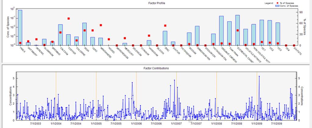
50 4.4.2 Source Profile Identification and Contribution Nine sources were identified for CAMS 312 and CAMS 60, based on the composition of the different species in it. The source profiles are: traffic, industrial, aged sea salt, biomass, roadside crustal, secondary sulfate II, secondary sulfate, crustal and secondary nitrate. The factors were similar for both the sites. The source profile and time series plot for the sources from the GUI is shown in Appendix B The source contribution and percentage of each factor for CAMS 312 and CAMS 60 are shown in figure 22and 23. It was identified from these figures that secondary sulfate and traffic are the two major contributors of PM 2.5 Figure 22 : Source contribution and percentages of each factors of CAMS

51 Figure 23 : Source contribution and percentages of each factors of CAMS Conditional Probability Function (CPF) CPF was also applied to the results from EPA PMF 3.0 to locate the source regions influencing the study region. The CPF applied to CAMS 312 showed a similar profile as the CPF for PMF 2. This was primarily due to the fact that the sources were identified as being similar. These source profiles and corresponding CPF are provided in Appendix B. CAMS 60 has a CPF profile slightly different from the one that was calculated using PMF2. Two new profiles identified by EPA PMF 3.0 are explained below and the rest are shown in Appendix B. 42

52 Figure 24: CPF plot for CAMS 60 for secondary sulfate II and road side crustal Secondary sulfate II is basically due to local anthropogenic activity, whereas road side crustal is usually produced due to traffic sources. The site is surrounded by roads and is in close proximity to Hinton Street which is to the south east of the site, The CPF plot shows the influence of road side crustal dust from Hinton Street and surrounding roads predominantly affecting the site. 43

53 4.5 Potential Source Contribution Factor (PSCF) Analysis PSCF analysis was used to understand the effects of long range transport affecting the Dallas urban airshed. The raw data analysis performed has shown that the air parcel gets transferred to Dallas from distant locations. Hence the PSCF analysis was necessary to locate and identify the influence of these upwind pollutant sources and source-rich regions. The sources typically identified as influence by long range transport of air pollution include biomass, secondary sulfate and crustal dust. PSCF performed on the source titled biomass burning identified Mexico and Central America as the primary location of sources, as shown in figures 25 and 26. Researchers have identified the impact of biomass burns from Mexico and Central America affecting urban airsheds in Texas (Karnae and John, 2011). Also, TCEQ has identified the transport of smoke plumes from Mexico and Central America using satellite imagery (TCEQ, 2012). Figure 25 : PSCF analysis of biomass burns on Dallas using CAMS 60 44

54 Figure 26 : PSCF analysis of biomass burns on Dallas using CAMS 312 Secondary sulfate is another species influenced by long range transport which occurs due to combustion related anthropogenic activities. The PSCF analyses using 5-day back trajectories are shown in figures 27 and 28. This indicates the transport of secondary sulfates from neighboring states such as Louisiana, and Arkansas and further upwind from the Mississippi River region and the Ohio River valley area. The urban and industrialized areas in these regions have a major impact on the air quality in Dallas. Both the figures show that Ohio River Valley acts as the main contributor of secondary sulfate identified in Dallas. Figure 27: PSCF analysis of secondary sulfates on Dallas using CAMS 60 45

55 Figure 28: PSCF analysis of secondary sulfates on Dallas using CAMS 312 The third type of long range transport affecting the urban airshed was crustal dust. A 12- day back trajectory was performed and it was identified that higher probability of contribution of crustal dust were transported from western regions of Africa during the sub-saharan desert storms. Figure 29 : PSCF plots for crustal dust showing that the dust is transported from Africa for CAMS 60 46

56 Figure 30 : PSCF plots for crustal dust showing that the dust is transported from Africa for CAMS 312 A 12-day back trajectory was required as it is the time required for air parcel to travel from Africa to Dallas. The intensity of the pollution subsides as it reaches Dallas but still there is a considerable amount which influences the air quality in Dallas. 47

57 CHAPTER 5 INTER-COMPARISON OF PMF 2 AND EPA PMF 3.0 MODEL RESULTS Using the PMF 2 and EPA PMF 3.0 models, source apportionment was performed for data set collected from CAMS 312 and CAMS 60. The sources identified were almost similar but there were some uncertainties in few of the sources identified by PMF 2. Tables 13 and14 show the factors identified by both the models along with their percentages and figures 30 and 31 is a graphical representation of the same set of results. Table 13: Comparison of source profiles identified from CAMS 312 by PMF 2 and EPA PMF3.0 CAMS 312 SOURCES PMF 2 EPA PMF Crustal 6.9% 2.2% Secondary Nitrate 10.3% 17.0% Industrial 7.8% 6.9% Road side Crustal 4.5% 7.2% Biomass 5.8% 4.3% Traffic 17.7% 21.75% Secondary Sulfate 31.3% 26.8% Secondary Sulfate II 10.9% 17.0% Aged Sea Salt 4.7% 3.5% 48

58 Percentage of conc. 35% 30% 25% 20% 15% 10% 5% 0% PMF 2 EPA PMF Crustal Secondary Nitrate Industrial Road Side Crustal Biomass Sources Traffic Secondary Sulfate Secondary Sulfate II Aged Sea Salt Figure 31 : Comparative illustration of source identified from CAMS 312 using PMF 2 and EPA PMF 3.0 Table 14: Comparison of source profiles identified from CAMS 60 by PMF 2 and EPA PMF 3.0 CAMS 60 SOURCES PMF 2 EPA PMF Crustal 13.5% 7.1% Secondary Nitrate 10.7% 8.2% Industrial 5.5% 6.9% Road Side Crustal - 4.9% Biomass 6.5% 6.0% Traffic 21.4% 20.9% Secondary Sulfate 34.8% 34.4% Secondary Sulfate II - 6.2% Aged Sea Salt 5.4% 5.4% Secondary Sulfate II comingled with industrial 2.4% - 49

59 Pecentage of Conc 40% 35% 30% 25% 20% 15% 10% 5% 0% PMF 2 EPA PMF Crustal Secondary Nitrate Industrial Road Side Crustal Biomass Sources Traffic Secondary Sulfate Secondary Sulfate II Aged Sea Salt Secondary Sulfate II comingled with industrial Figure 32: Comparative illustration of source identified from CAMS 60 using PMF 2 and EPA PMF 3.0 EPA PMF 3.0 had 9 factors for CAMS 60 but using PMF 2 it only identified 8 factors for the same site. There was a commingling of two sources at this site as shown by PMF2, whereas PMF 3 clearly distinguished between the two sources separately and thus identifying 9 factors. Two new factors for CAMS 60 are secondary sulfate II and road side crustal dust. The mass percentages identified by both models for similar sources were comparable; there were instance of higher value prediction by PMF 2. Figures 31 and 32 show the graphical comparison of sources identified by both the models. EPA PMF 3.0 was very user friendly and the analysis is lot faster. Robust approaches were taken in species classification providing the user to understand the goodness of each species. In the case of PMF2, only signal to noise ratios were used for species classification and which at times may not be an acceptable methodology. Weekend-weekday comparison and seasonal analysis was performed using the results from both the models for both the sites. 50

60 Average PM 2.5,µgm PMF2_WeekEnd PMF2_WeekDay EPA PMF_WeekEnd EPA PMF_WeekDay Traffic Secondry sulfate II Biomass Road Side Crustal Aged Sea Salt Sources Crustal Secondary Nitrate Industry Secondary sulfate Figure 33: Weekend-weekday analysis at CAMS 312 using PMF2 and EPA PMF 3.0 Average PM 2.5,µgm EPA PMF_WeekEnd PMF2_WeekEnd EPA PMF_WeekDay PMF2_WeekDay Traffic Industrial Biomass Crustal Sources Secondary Nitrate Secondary Sulfate Aged Sea Salt Figure 34 : Weekend-weekday analysis for common sources at CAMS 60 using PMF2 and EPA PMF 3.0 From the weekend and weekday analysis it was noted that the traffic, industrial and roadside crustal dust sowed distinct weekday-weekend day characteristics. These sources showed higher values during the weekdays and lower levels during the weekend days. Figures 33 and 34 shows the weekend-weekday analysis for the common sources apportioned by EPA PMF 51

61 3.0 and PMF2 at CAMS 312 and CAMS 60. Appendix C has the weekend-weekday graphs for the unique sources identified at CAMS 60. A detailed seasonal analysis was conducted and it was found to be very effective since it provided the variation of the sources during each season. The secondary sulfate showed an increase during the summers than other months especially the winter months. During the winter, the concentration of secondary sulfate for CAMS 312 and CAMS 60 predicted by both the models were found to be low as shown in figures 35(a) and 36(a) for CAMS312 and CAMS 60, respectively. Table 15 shows the amount of concentration during the winter months for both the sites. Following the winter months, the concentrations increased and reached a peak level during summer, almost twice that of winter as shown in figures 35(c) and 36(c) for CAMS 312 and CAMS 60, respectively. Table 15 shows the seasonal distribution However, in the case of secondary nitrates an opposite trend was observed; higher concentrations in the colder seasons and dropping when it approaches the hotter seasons. The trend for that is shown in figures 35(a) and (c) and figures 36 (a) and (c) for CAMS 312 and CAMS 60, respectively. Table 15 shows the seasonal concentration distribution for both the sites. It also identified that crustal dust levels increases during summer and tends to be lower during the winter months. Roadside crustal dust follows a similar pattern as that of the traffic and this was also one of the strong evidence that the source identification was solid. 52

62 Table 15: Variation in concentration of the sources in hot and cold seasons Source Summer PMF2 Winter- PMF2 Secondary Sulfate Secondary Nitrate CAMS 312 CAMS 60 CAMS 312 CAMS 60 Summer EPA PMF CAMS CAMS Winter- EPA PMF CAMS 312 CAMS Crustal Average PM 2.5,µgm Secondary Sulfate II Traffic Seasonal Comparison -Winter Roadside Crutal Biomass Secondary Nitrate Industry Secondary Sulfate EPA PMF_Winter PMF2_winter Aged sea Salt Crustal (a) Average PM 2.5,µgm Secondary Sulfate II Traffic Seasonal Comparison -Spring Roadside Crutal Biomass Secondary Nitrate Industry Secondary Sulfate EPA PMF_ Spring PMF2_Spring Aged sea Salt Crustal (b) Average PM 2.5,µgm Secondary Sulfate II Traffic Seasonal Comparison -Summer Roadside Crutal Biomass Secondary Nitrate Industry Secondary Sulfate EPA PMF_Summer PMF2_Sumer Aged sea Salt Crustal (c) 53

63 Average PM 2.5,µgm Secondary Sulfate II Traffic Roadside Crutal Seasonal Comparison -Fall Biomass Secondary Nitrate Industry Secondary Sulfate EPA PMF_Fall PMF2_Fall Aged sea Salt Crustal (d) Figure 35: Seasonal analysis for CAMS 312 inter-comparison of results for sources where (a) winter (b) spring (c) summer (d) fall Average PM 2.5,µgm Seasonal Comparison-Winter EPA PMF_Winter PMF2_Winter Traffic Biomass Secondary Nitrate Industry Secondary Sulfate Aged sea Salt Crustal (a) Average PM 2.5,µgm -3 Average PM 2.5,µgm Seasonal Comparison-Spring EPA PMF_Spring PMF2_Spring Traffic Biomass Secondary Nitrate Industry Secondary Sulfate Aged sea Salt Crustal Seasonal Comparison-Summer EPA PMF_Summer PMF2_Summer Traffic Biomass Secondary Nitrate Industry Secondary Sulfate Aged sea Salt Crustal (b) (c) 54

64 Average PM 2.5,µgm Seasonal Comparison-Fall EPA PMF_Fall PMF2_Fall Traffic Biomass Secondary Nitrate Industry Secondary Sulfate Aged sea Salt Crustal (d) Figure 36: Seasonal analysis for CAMS 60 inter-comparison of results for common sources where (a) winter (b) spring (c) summer (d) fall Overall, the PMF2 consistently predicted slightly higher values when compared to EPA PMF 3.0 and this may be because the model was not able to eliminate the weak species which had limited or lesser influence on the apportioned PM 2.5 levels. 55

65 CHAPTER 6 CONCLUSION AND RECOMMENDATIONS Source apportionment analysis of measured PM 2.5 concentrations in Dallas, Texas was performed with data collected from two TCEQ air quality monitoring sites (CAMS 312 and CAMS 60) and by using two positive matrix factorization models EPA PMF 3.0 and PMF 2. The raw data analysis of the average PM 2.5 concentrations showed a decreasing trend over the span of 7 years, also its influence was found to be higher during the summer season when compared to other seasons. This study has concluded that the urban airshed of Dallas is continuously affected by both local sources and long range transport of air pollution. Two major sources identified to affect this urban area included traffic (17-22% of the apportioned PM 2.5 ) and secondary sulfate (26-35%). Other sources identified were crustal ( %), secondary nitrate ( %), industrial ( %), road side crustal ( %), biomass burns ( %), aged sea salt ( %) and secondary sulfate II (6.2%-17.0%). Conditional probability function (CPF) was used to identify the spatial location of these sources. Using CPF, It was easier to identify local source regions affecting the receptor site. PSCF was employed to study the influence of three major source categories (secondary sulfates, biomass burns and crustal dust) influenced by the long range transport of pollution. Secondary sulfates were found to be transported all the way up from Ohio River Valley and from the neighboring states surrounding the Dallas urban airshed. Biomass burns from Central America and Mexico also influenced the Dallas urban airshed. Higher loadings of crustal dust were associated with sub-saharan desert storms as a result of the transport of crustal dust from Africa to Texas and beyond. 56

66 Inter-comparison of the results from the two models has helped in the understanding of their robustness. As hypothesized, EPA PMF 3.0 was found to be more user-friendly, more accurate and was able to discern the sources better than PMF 2. Time taken to complete the analysis was less while using EPA PMF 3.0. Various analyses such as weekend-weekday, seasonal and the annual analysis were readily available on the GUI of EPA PMF 3.0 which helped reduce time for completing the analysis. Seasonal analysis showed that secondary sulfates are high during summer and are lower during winter time. This could be indirectly due to the high demand of electricity during summer and the coal fired power plants work on maximum load to meet the increasing demand, thus increasing the PM pollution. Secondary nitrate showed an opposite trend as they were higher in winter and low during summer. Crustal dust was found to be high during the summer months. PMF 2 has consistently apportioned more mass from the major sources when compared to EPA PMF 3.0. From this study it was identified that secondary sulfate and traffic have the highest influence on the air quality in Dallas. It is known that prolonged exposure to PM 2.5 can affect health conditions. Therefore it is recommended that the policy makers should bring in effective emission control strategies to mitigate the impact of these sources. The results of this study could help establish proper air quality policies, regulations and new standards in air quality permits for industries, thus reducing the health and environmental hazards caused by the criteria pollutant PM

67 APPENDIX A GRAPHS AND TABLES USED IN PMF 2 ANALYSIS 58

68 Table A - 1 and A - 2 are the species classification identified by PMF2 for CAMS 312 and CAMS 60. There were 25 strong and 10 weak species for CAMS 312 and 28 and 13 for CAMS 60. Table A - 1: Species classification for CAMS 312 using PMF 2 Variable No Species Classification Strong 25 PM 2.5, Aluminum, Bromine, Calcium, Copper, Chlorine, Iron, Phosphorous, Titanium, Silicon,Zinc, Sulfur, Potassium, Sodium, Ammonium Ion, Sodium Ion, Potassium Ion, Elemental Carbon, Non-Volatile Nitrate, Sulfate,OC1,OC2,OC3 and OC4 Weak 10 Arsenic, Barium, Chromium, Lead, Manganese, Nickel, Magnesium, Vanadium, Strontium and Yttrium Table A - 2: Species classification for CAMS 60 using PMF2 No Species Strong 28 PM 2.5,Antimony,Arsenic,Aluminum, Barium, Bromine, Cadmium, Calcium, Chromium, Cobalt, Copper, Chlorine, Cerium, Cesium, Europium, Gallium, Iron, Hafnium, Lead, Indium, Manganese, Iridium, Molybdenum, Nickel, Magnesium, Mercury, Gold, Lanthanum, Niobium, Phosphorous, Selenium, Tin, Titanium, Samarium, Scandium, Vanadium, Silicon, Silver, Zinc, Strontium, Sulfur, Tantalum, Terbium, Rubidium, Potassium, Yttrium, Sodium, Zirconium, Wolfram, Ammonium Ion, Sodium Ion, Potassium Ion, Organic Carbon, Total Nitrate, Elemental Carbon, Volatile Nitrate, Non-Volatile Nitrate, OC1, OC2, OC3, OC4 and Sulfate Weak 13 Arsenic, Barium, Chromium, Europium, Nickel, Magnesium, Mercury, Lanthanum, Selenium, Samarium, Vanadium, Strontium, Terbium 59

69 Figure A - 1 and A - 2 are other Fpeak analysis performed for PMF2 to understand the number of sources in that particular site. Figure A - 1: Fpeak analysis for 7 and 8 factors of CAMS 312 Figure A - 2: Fpeak analysis for 9 and 10 factors of CAMS 60 60

70 Figure A - 3 shows various source profiles identified from CAMS 312. Each of the figures shows the composition of each source. Mass Fraction Traffic 1 Industrial Mass Fraction Mass Fraction Aged SeaSalt Mass Fraction Biomass Mass Fraction Road side Crustal Al Br Ca Cu Cl Fe P Ti Si Zn S K Na NH Na+ K+ OC EC NO32 SO4 OC1 OC2 OC3 OC4 As Ba Cr Pb Mn Ni Mg V Sr Y 61

71 Secondary Sulfate II Mass Fraction Secondary Sulfate Mass Fraction Mass Fraction Crustal Mass Fraction Secondary Nitrate Al Br Ca Cu Cl Fe P Ti Si Zn S K Na NH Na+ K+ OC EC NO32 SO4 OC1 OC2 OC3 OC4 As Ba Cr Pb Mn Ni Mg V Sr Y Figure A - 3 : Source profile for CAMS

72 Figure A - 4 shows various source profiles identified from CAMS 60. Each of the figures shows the composition of each source. There were 8 source profiles corresponding to the sources identified. Mass Fraction Secondary sulfate Mass Fraction Aged sea salt 1 Secondary sulfate II comingled with industrial Mass Fraction Mass Fraction Crustal 63

73 Mass Fraction Traffic Al Br Ca Cu Cl Fe Pb Mn Ti Si Zn S K Na NH4+ Na+ K+ OC TN EC VN NO32 OC1 OC2 OC3 OC4 SO4 Ar Ba Cr Eu Ni Mg Hg La Se Sm V Sr Tb Figure A - 4: Source profile for CAMS 60 Mass Fraction Industrial Mass Fraction Biomass 1 Secondary nitrate Mass Fraction Al Br Ca Cu Cl Fe Pb Mn Ti Si Zn S K Na NH4+ Na+ K+ OC TN EC VN NO32 OC1 OC2 OC3 OC4 SO4 Ar Ba Cr Eu Ni Mg Hg La Se Sm V Sr Tb Figure A - 5: Source profile for CAMS 60 64

74 Figure A - 5 represents the weekend weekday analysis of each source of CAMS 312 where sources like traffic are high on weekdays where as on weekends they are lower. Roadside crustal dust follows the similar pattern as it is influenced on how the traffic flows. Average PM 2.5,µgm Traffic WeekEnd WeekDay (a) Average PM, μgm Industrial WeekEnd WeekDay (b) Average PM, μgm Aged sea salt WeekEnd WeekDay (c) Average PM, μgm Biomass WeekEnd WeekDay (d) Average PM, μgm Road side crustal WeekEnd WeekDay (e) Average PM, μgm Secondary sulfate II WeekEnd WeekDay (f) 65

75 Average PM, μgm Secondary sulfate WeekEnd WeekDay (g) Average PM, μgm WeekEnd Crustal WeekDay (h) 0.8 Secondary nitrate Average PM, μgm WeekEnd WeekDay (i) Figure A - 6.: Weekend weekday analysis of each sources of CAMS 312 Figure A - 6 represents the weekend weekday analysis of each source of CAMS 60 where traffic is high on weekends and whereas lower on weekdays they are lower. This could be influence of restaurants and malls which are there in that region and people use them more on weekends. Industrial source is high on weekdays as they are working on full capacity. Average PM 2.5,µgm -3 Secondary sulfate II co-mingled with industrial WeekEnd WeekDay (a) Average PM 2.5,µgm Biomass Weekend Weekday (b) 66

76 Average PM 2.5,µgm Secondary Nitrate Weekend Weekday (c) Average PM 2.5,µgm Weekend Industry Weekday (d) Average PM 2.5,µgm Secondary sulfate Weekend Weekday Average PM 2.5,µgm Aged sea salt Weekend Weekday (f) (e) Average PM 2.5,µgm Weekend Crustal Weekday (g) Average PM 2.5,µgm Traffic Weekend Weekday (h) Figure A - 7 Weekend weekday analysis of each sources of CAMS 60 67

77 Average PM 2.5,µgm Traffic Winter Spring Summer Fall Seasons (a) Average PM 2.5,µgm Industrial Winter Spring Summer Fall Seasons (b) Average PM 2.5,µgm Aged sea salt Winter Spring Summer Fall Aged Sea Salt (c) Average PM 2.5,µgm Biomass Winter Spring Summer Fall Seasons (d) Average PM 2.5,µgm Road Side Crustal Winter Spring Summer Fall Seasons (e) Average PM 2.5,µgm Secondry sulfate II Winter Spring Summer Fall Seasons (f) Average PM 2.5,µgm Secondary sulfate Winter Spring Summer Fall Seasons (g) Average PM 2.5,µgm Crustal Winter Spring Summer Fall Seasons (h) 68

78 Average PM 2.5,µgm Secondary nitrate Winter Spring Summer Fall Seasons (i) Figure A - 8 : Seasonal analysis for each source of CAMS 312 Average PM 2.5,µgm Secondary sulfate Winter Spring Summer Fall Seasons Average PM 2.5,µgm Aged Sea Salt Winter Spring Summer Fall Seasons (a) (b) Average PM 2.5,µgm Secondary Sulfate II Co-mingled with industrial Winter Spring Summer Fall Seasons Average PM 2.5,µgm Crustal Winter Spring Summer Fall Seasons (c) (d) Average PM 2.5,µgm Traffic Winter Spring Summer Fall Seasons (e) Average PM 2.5,µgm Industrial Winter Spring Summer Fall Seasons (f) 69

79 Average PM 2.5,µgm Biomass Winter Spring Summer Fall Seasons (g) Average PM 2.5,µgm Secondary Nitrate Winter Spring Summer Fall Seasons (i) Figure A - 8 : Seasonal analysis for each source of CAMS 60 Figure A - 7 and A - 8 shows the seasonal analysis for CAMS 312 and CAMS60 respectively. Secondary sulfates are high on summer and low in winter and other way secondary nitrate is low in summer and high in winter. 70

80 APPENDIX B GRAPHS AND TABLES USED IN EPA PMF 3.0 ANALYSIS 71

81 Figure B-1 gives the list of species which are classified as strong, weak and bad based on various analyses performed. Figure B - 1: CAMS 312 list of species (left) and CAMS 60 list of species, output from EPA PMF 3.0 GUI 72

82 Figure B - 2 shows the residual analysis of bromine and it was classified as weak based on this distribution. Whereas figure B - 3 was the residual analysis of zirconium, the distribution was poor hence it was classified as bad. Figure B - 2 : Residual analysis output of bromine from EPA PMF 3.0 GUI for CAMS 312 Figure B - 3: Residual analysis output of zirconium from EPA PMF 3.0 GUI for CAMS

83 Figure B - 4 and B - 5 illustrate the O/P scatter plot for nickel and gold,the weak and bad species in the species list. Figure B - 4 : O/P scatter plot for nickel from EPA PMF 3.0 of CAMS 312 Figure B - 5 : O/P scatter plot for gold from EPA PMF 3.0 of CAMS

84 Figure B 6 and B - 7 gives output from EPA PMF 3.0 which gives the concentration and percentage of species for CAMS 312 and CAMS 60 respectively along with the time series which shows the variation of that source based on time. (a) (b) (c) 75

85 (d) (e) (f) 76

86 (g) (h) Figure B - 6: Source profiles and time series analysis for CAMS 312 from GUI, where (a) Traffic (b) Secondary sulfate II (c) Road side crustal (d) Secondary nitrate (e) Industry (f) Crustal (g) Biomass (h) Aged sea salt (i) Secondary sulfate (i) 77

87 (a) (b) (c) 78

88 (d) (e) (f) 79

89 (g) (h) Figure B - 7: Source profiles and time series analysis for CAMS 60 from GUI where (a) Secondary sulfate II (b) Traffic (c) Road side crustal (d) Biomass (e) Secondary nitrate (f) Industry (g) Secondary sulfate (h) Aged sea salt (i) Crustal (i) 80