Wireless Magnetic Sensor Applications in Transportation Infrastructure. Rene Omar Sanchez

Transcription

1 Wireless Magnetic Sensor Applications in Transportation Infrastructure by Rene Omar Sanchez A dissertation submitted in partial satisfaction of the requirements for the degree of Doctor of Philosophy in Engineering - Mechanical Engineering in the Graduate Division of the University of California, Berkeley Committee in charge: Professor Roberto Horowitz, Chair Professor J. Karl Hedrick Professor Pravin Varaiya Fall 22

2 Wireless Magnetic Sensor Applications in Transportation Infrastructure Copyright 22 by Rene Omar Sanchez

3 Abstract Wireless Magnetic Sensor Applications in Transportation Infrastructure by Rene Omar Sanchez Doctor of Philosophy in Engineering - Mechanical Engineering University of California, Berkeley Professor Roberto Horowitz, Chair Intelligent Transportation Systems (ITS) are cost-effective measures to manage congestion due to increasing demand by improving the efficiency of existing transportation infrastructure. Traffic detection and surveillance play a pivotal role in deploying these technologies in the field. This dissertation continues the work that has been done in recent years in relation to the use of wireless magnetic sensor networks in transportation systems. As part of the effort to improve vehicle detection system technologies so that better management strategies can be implemented in the field, the work presented here focuses on advancing the use of wireless magnetic sensors in Intelligent Transportation Systems. This dissertation addresses improvements in algorithmic tools that advance the use of wireless magnetic sensors for both freeways and arterials. The applications addressed here include on-ramp queue estimation, arterial link vehicle-count, travel time estimation on heavily congested arterial streets, travel time and link vehicle-count in freeways, truck re-identification along long freeway segments, as well as cost-effective vehicle classification. The overall goal of this dissertation is to advance the use of these basic detection technologies to roles that extend beyond basic vehicle detection. A vehicle re-identification system, which relies on matching vehicle signatures from wireless magnetic sensors is modified to improve its performance for stop-and-go traffic conditions and is extended so that it can be used for truck re-identification along long freeway segments. The modifications to the algorithm address problems observed when vehicles stop or accelerate/decelerate as they go through the sensors. The modified system was tested to ensure that it overcame the deficiencies imposed by the original system. The extension of the vehicle re-identification system, presented as the iterative vehicle re-identification system, addresses traffic dynamics observed when vehicles travel along long road segments, in particular, vehicle overtaking. The system was tested extensively to ensure that it can be deployed for truck re-identification along long freeway segments, e.g., in between weigh-in-motion (WIM) stations. A link vehicle-count and a travel time estimator based on flow-measurements and vehicle reidentification data were studied at a freeway on-ramp, arterial segments as well as at freeway segments. The results show that the estimators are reliable and accurate, and are suitable for real-

4 time traffic responsive management strategies that require precise link vehicle-count and/or vehicle travel time information, such as ramp metering, speed control and traffic intersection control. Vehicle classification, which utilizes a single wireless magnetic sensor installed in the middle of a freeway lane is also presented. The approach uses a two stage binary support vector machine (SVM) classifier based on features extracted from vehicle signatures. This is a cost effective classification system that uses a small subset of data efficiently extracted from the magnetic signal measured by the sensor. The results showed that vehicles can be reliably and accurately classified into passenger vehicles and trucks, and once trucks are extracted, this group can be further divided, with lower accuracy and consistency, into two groups: small trucks and large trucks. Finally, this dissertation presents a systematic tool for tuning vehicle re-identification parameters and evaluating performance. This tool uses different plots, metrics and algorithms to evaluate the output of the vehicle re-identification algorithm as well as estimates based on it, i.e., link vehicle-count and vehicle travel time. 2

5 To my family, i

6 ii Contents Contents List of Figures List of Tables Acknowledgements ii v x xii Introduction 2 Background and Review of Previous Work 6 2. Traffic Detection Technologies and Traffic State Measurement Traffic Surveillance Technologies Traffic State Measurement Wireless Magnetic Sensors Vehicle Detection System Vehicle Re-Identification Using Wireless Magnetic Sensors Vehicle Magnetic Signature Vehicle Re-Identification Algorithm Summary Travel Time Estimation and Vehicle Link-Count Using Wireless Magnetic Sensors 23 Travel Time Link Vehicle-Count Analysis of On-Ramp Queue Estimation Methods Introduction Queue Estimation Methods Test Site Vehicle Detection System Ground Truth Data Collection Queue Estimation Results Occupancy-Based Queue Estimation Method Queue Estimation Method Based on Vehicle Counts Queue Estimation Method Based on Speed Queue Estimation Method Based on Vehicle Counts and Speed

7 iii Queue Estimation Method Based on Vehicle Re-Identification Sources of Error Discussion Vehicle Re-Identification: Algorithm Revision, Modifications and Performance Analysis Introduction Data Ground Truth Data Vehicle Detection System Data Vehicle Subsets Chosen Vehicles Vehicle Re-Identification Method Revision Signal Processing Step Revision Vehicle Signatures Revision Matching Step Revision Vehicle Re-Identification Method Modifications Signal Processing Algorithm Modification Signal Processing Improvements Matching Algorithm Modification Vehicle Re-Identification Results Default vs Iterative µ f, σ f, µ g, σ g Results Iterative µ f, σ f, µ g, σ g with varying β Results Application: Link Vehicle-Count based on Vehicle Re-Identification Improved On-ramp Queue Estimation Arterial Link Vehicle-Count Estimation: Original vs Modified Method Discussion Arterial Travel Time Estimation based on Vehicle Re-Identification: Performance Analysis 7 5. Introduction Test Site Vehicle Detection System Data Ground Truth Data Vehicle Detection System Data Ground Truth and Vehicle Detection System Data Analysis Lane Changing First In, First Out (FIFO) Condition Travel Time by Vehicle Category Travel Time Results Discussion

8 iv 6 Wireless Magnetic Sensor Applications for Freeways Introduction Test Sites Pinole Test Site Caldecott Tunnel Test Site Vehicle Re-Identification Pinole Test Site Analysis Caldecott Tunnel Analysis Vehicle Classification Vehicle Classes Vehicle Data Sets Support Vector Machine Results Truck Re-Identification Along Long Freeway Segments Truck Data Sets Vehicle Re-Identification Algorithm Extension: Iterative Method Analysis on Overtaking: Artificial Shuffling Analysis on Overtaking: Shuffling Based on Real Data Discussion Vehicle Re-Identification Systems Tuning Tool Introduction Tool Overview Test Site Tool Components Peak Analysis Component Distance Matrix Component f and g Component Matching Algorithm Component Matching Algorithm Plots Component Sensor Pair Minimum Distance Frequency k-shortest Paths Component Matched Signatures Subset Analysis Component Discussion Conclusions 5 Bibliography 55

9 v List of Figures 2. Upstream and downstream middle sensor raw signals with extracted peak value sequences (dots) Upstream and downstream middle sensor signature slices Third vehicle upstream and downstream signatures (five vehicle example) Fifth vehicle upstream and downstream signatures (five vehicle example) First vehicle upstream signature and fourth vehicle downstream signature (five vehicle example) Five vehicle example (a) distance matrix, (b) distance matrix gray scale heat map and (c) f and g pdfs Edit graph edge weights (five vehicle example) Shortest paths (five vehicle example) k-shortest paths (five vehicle example) Link vehicle-count based on vehicle re-identification by signature matching (colored squares represent vehicles that have been matched before t) Photos showing (a) aerial view of Hegenberger on-ramp with saturated queue, (b) side view of Hegenberger on-ramp with saturated queue, and (c) arterial streets and intersections around Hegenberger on-ramp Wireless magnetic sensors (shown as blue dots) setup for different queue estimation methods at a single lane freeway on-ramp Photos showing (a) Hegenberger on-ramp entrance (bottom square) and exit (top square), (b) vehicle detection system installation at ramp entrance, and (c) sensor array installation at ramp exit (Re-Id = re-identification) Configuration of wireless magnetic sensors at entrance of Hegenberger on-ramp (a) Video camera recording vehicles leaving on-ramp, (b) cassette video camera recording vehicles entering on-ramp, and (c) video camera to capture vehicle behavior and queue dynamics (top) Occupancy and queue length graphed as a function of time of day, and scatter plots of queue length versus occupancy for (bottom, left) 5-s, (bottom, middle) 3-s, and (bottom, right) 6-s intervals (top) Graph of queue length based on ground truth data and arrays raw data

10 vi 3.8 (left) Graph of entrance vehicle counts based on ground truth, entrance array and SL, SL2, ST, and ST2 sensors, and (right) table showing total entrance vehicle counts between 6.3 h and 7.6 h (top) Speed-trap measurements and ground truth speed graphed as a function of time of day, (bottom, left) scatter plot of queue lengths versus speed at entrance of on-ramp, and (bottom, right) scatter plot of queue lengths versus three trailing point moving average of speed (top) Queue length estimate for every speed measurement and (bottom) speed based queue estimate for a 3-s calculation interval Queue estimation based on vehicle counts and speed (top) with no restrictions and (bottom) with estimates constrained to [,25] Queue length based on vehicle re-identification versus time of day (a) Motorcycle bypassing queue, (b) vehicle bypassing queue, (c) large truck entering on-ramp, (d) off-centered vehicles with respect to lane, and (e) adjacent vehicles simultaneously stopped on top of leading and trailing speed-trap sensors Original distance matrix for the (left) 23 chosen vehicles (right) complete vehicle data set Vehicle k = 527 two signature slices at the entrance and exit arrays (a) raw peak values, (b) processed for original distance calculation (c) processed for modified distance calculation Modified distance matrix for the (left) 23 chosen vehicles (right) complete vehicle data set Comparison between the (top) original and the (bottom) modified distance method (left) Matched vehicles as a function of β, (middle) % of uncongested mismatched vehicles as a function of β and (right) % of congested mismatched vehicles as a function of β Hegenberger on-ramp queue length estimates using β =.5 with (top) the original method and default f and g, (middle) original method and Hegenberger f and g and (bottom) modified method and Hegenberger f and g Hegenberger on-ramp (top) queue estimates and (bottom) travel time estimates from Monday, March 2, to Sunday, March 27, Queue estimates at the Hegenberger on-ramp on Tuesday, March 22, 2, from 5.25 h to 8.25 h Queue estimates at the Hegenberger on-ramp on Saturday, March 26, 2, from 6.5 h to 7.83 h mile segment of San Pablo Avenue in Berkeley, CA: (a) aerial view with long queues and (b) segment schematic Link vehicle-count estimates using vehicle re-identification with (top) the original method and (bottom) the modified method mile segment of 34th Street in New York City

11 vii 5.2 Segment (a) start (upstream) location and (b) end (downstream) location Camera recording vehicles at (a) the START location and at (b) the END location Color map of the ground truth mapping k l for the slow f ast link: (left) complete vehicle sequence (right) largest vehicle sequence satisfying FIFO Ground truth travel time frequency distribution by vehicle group: (top) taxis and buses and (bottom) vehicles except taxis and buses Travel time frequency distribution for (top) the ground truth, (b) the original method and (c) the modified method Empirical cumulative travel time distribution for the ground truth, the original method and modified method (a) Pinole test site and #58 Caltrans WIM station (b) configuration of wireless magnetic sensors at the Pinole test site (a).68-mile Caldecott Tunnel segment in California State Route 24, (b) west vehicle detection system installation and (c) east vehicle detection system installation (left) Distance matrix for the P2 data set and (right) matched vehicles matrix for the P2 data set Results at the Pinole test site for the P2 data set C data set results C2 data set results C3 data set results C4 data set results C5 data set results C5 data set (left) distance matrix and (right) matched vehicles matrix FHWA 3-category scheme for vehicle classification (image from [42]) Distance and matched vehicles matrices for (a) T data set, (b) upstream T data set vs downstream P2 data set and (c) T2 data set Matched vehicles distribution (m=) for different random matrix D randg sizes: (left) 73x73 (middle) 73x672 (right) 49x Normalized matching rate distributions (m=) for different β values and for different random matrix D randg sizes: (top) 73x73 (middle) 73x672 (bottom) 49x Normalized matching rate distributions (m=) for different σ g and for different random matrix D randg sizes: (top) 73x73 (middle) 73x672 (bottom) 49x Color map of the (left) maximum number of matched vehicles and (right) acceptable matching rate lower bound, from matching results distributions based on m= N M random distance matrices D randg, for N = and M = Number of vehicles to overtake o discrete probability density function Downstream signature sequence shuffling (five vehicle example) (a) Scenario, (b) Scenario 2 and (c) Scenario Evolution of vehicle re-identification results for scenario for p o= and c=5 (results listed in Table 6.4)

12 viii 6.2 (top) Travel time and (bottom) time-space diagram for 49 successive departing trucks at the upstream WIM station (from [2] truck data set) Evolution of the vehicle re-identification results for truck shuffling based on real data Vehicle re-identification tool data flow mile Missouri arterial segment with 3 sensor arrays forming 2 array links Average number of peaks as a function of sensor for (left) segment 79 and (right) segment Number of peaks distribution (x+y+z) for each of the sensors in (left) segment 79 and (right) segment Number of peaks as a function of signature for (left) segment 79 and (right) segment Number of peaks per signature distribution for (left) segment 79 and (right) segment Distance matrix for (left) segment 79 and (right) segment Distance matrix f and g distributions for (left) segment 79 and (right) segment Linear assignment matched vehicles matrix for (left) segment 79 and (right) segment Linear assignment f and g distributions for (left) segment 79 and (right) segment Matching results for the four different sets of f and g parameters for (left) segment 79 and (right) segment Travel time empirical cumulative distribution function (CDF) for the four different sets of f and g parameters for (left) segment 79 and (right) segment Edit graph, G (2,2), shortest path for the four different sets of f and g parameters for (left) segment 79 and (right) segment Matched vehicles travel time and signature distance distributions using the linear assignment f and g parameters for (left) segment 79 and (right) segment Travel time, link vehicle-count and matching rate based on matching results using linear assignment f and g parameters for (left) segment 79 and (right) segment Sensor pair minimum distance frequency plot based on linear assignment f and g matching results for (left) segment 79 and (right) segment Shortest path matched vehicles matrix based on linear assignment f and g parameters for (left) segment 79 and (right) segment shortest paths incidence matrix based on linear assignment f and g parameters for (left) segment 79 and (right) segment k=5 common matched vehicles matrix based on linear assignment f and g parameters for (left) segment 79 and (right) segment Matched signature pair producing a relatively small distance for (left) segment 79 and (right) segment Matched signature pair producing a relatively intermediate distance for (left) segment 79 and (right) segment

13 7.22 Matched signature pair producing a relatively large distance for (left) segment 79 and (right) segment ix

14 x List of Tables 3. Table showing total vehicle counts for ground truth and arrays data between 6.3 h and 7.6 h chosen vehicles Different f and g statistics for the original and modified signal processing methods Matching results using the default and iterative f and g from Table 7.2 for the original and modified method Ground truth and matching results using µ f =.8, σ f =.7, µ g =.6, σ g =.2 and β = Vehicle counts based on ground truth and sensor arrays data Chosen vehicles Ground truth data by vehicle type Matching results comparison Vehicle re-identification results for the Pinole test site on April 2, Vehicle re-identification results for the Caldecott Tunnel test site Distribution of vehicle classes in data set R Distribution of vehicle classes in data set R Distribution of vehicle classes in data set R Single sensor magnetic signature features per component (x: n=, y: n=2 and z: n=3) Classification results: R data set Classification results: R and R2 data sets Classification results: R and R3 data sets Distribution of vehicle classes in data set T Distribution of vehicle classes in data set T Mean µ and standard deviation σ of the distribution of matched vehicles produced from m randomly generated distance matrices D randg Total iterative results vs iterative results with automatic stopping criteria (c=5, size(d) = 49x49) Iterative vehicle re-identification results for scenario for p o= and c=

15 xi 6.5 Total iterative results vs iterative results with automatic stopping criteria (c=, size(d) = 73x672) Total iterative results vs iterative results with automatic stopping criteria (c=, size(d) = 73x3) Total iterative results vs iterative results with automatic stopping criteria (c=5, size(d) = 24x32) Iterative vehicle re-identification results for scenario 3 for p o= Iterative vehicle re-identification results for truck shuffling based on data from [2] Sensor arrays vehicle count on August 3, 2 from 5 p.m. to 6 p.m. (afternoon peak traffic) Sets of f and g parameters for segment 79 and segment

16 xii Acknowledgments Completing my Ph.D. studies would have not be possible without the constant support and love from my parents. I have also been fortunate to have Pamela, Julieta and Sebastian in my life, and I am grateful for their encouragement and support. I also thank my aunts Lulu and Totoy for their love. Special thanks to Professor Roberto Horowitz and Professor Pravin Varaiya for their patience, advice and encouragement over these years at UC Berkeley. I also take this opportunity to thank Professor J. Karl Hedrick, for serving in my dissertation and qualifying exam committee. I thank my friends at Berkeley, who have made my graduate life memorable. Ajith Muralidharan and Gunes Dervisoglu have been wonderful friends, and have been instrumental in the completion of my graduate studies. Thanks to Hector Mendoza and Jorge Robles for being great friends and for taking the time to read this dissertation and providing me with valuable comments and suggestions. I also want to thank Alex Kurzhanskiy, Gabriel Gomes and Ram Rajagopal, who have been exceptional role models and have been influential in shaping me as a researcher. I thank Christopher Flores for being a great mentor to me, and for his valuable involvement and help in many of the studies presented in this dissertation. This research was funded by Caltrans and the National Science Foundation. I also acknowledge the Alfred P. Sloan Scholarship for providing support to conduct part of this research.

17 xiii

18 Chapter Introduction Traffic congestion is a very large problem, and has been increasing across the world, particularly in cities with large and growing populations. Transportation agencies are unable to keep up with the increase in demand, especially at peak commuting times, due to deficient infrastructure, lack of space or funds for infrastructure expansion, and/or poor traffic management. According to the 2 Urban Mobility Report [7], in U.S. urban areas, congestion led to an increase on the average yearly delay per auto commuter from about 4 hours in 982, to about 34 hours in 2. This is not only an appreciable increase in delay to the average commuter, but also a significant increase in costs related to vehicle operating expenses (e.g., wasted fuel and wear), stress on transportation infrastructure, and environmental degradation as the result of significant pollution emissions. Strategic infrastructure expansion helps reduce or contain traffic congestion in metropolitan areas, but it is usually not enough, and alternative measures are needed. Intelligent Transportation Systems (ITS) emerged as cost-effective measures to accommodate increasing demand and manage congestion by improving the efficiency of existing transportation infrastructure. Here is where traffic surveillance technologies play a key role. In recent years, transportation agencies have seen the usefulness of data collection and archiving tools such as the Caltrans Performance Measurement System (PeMS) [4]. These systems store and process traffic data from roadway detectors installed throughout a traffic network. PeMS has proven extremely useful for real-time monitoring of traffic conditions, as well as for the analysis of the performance of highway systems in California. Having access to such a database has also allowed researchers and traffic engineers around the world to develop reliable tools for quantitative assessment of congestion relief strategies such as demand and incident management, traffic control, and traveler information. For example, historical data is used for calibration and validation of traffic simulators used in studies that address concerns about new control strategies, infrastructure expansion plans, or emergency management strategies without expensive and time consuming validation efforts in the field. PeMS illustrates the value of having quick and easy access to traffic data

19 2 for the advancement of ITS measures that increase transportation systems efficiency. However, it is well known that limitations of systems like PeMS are often associated with data availability and quality. Data are not reliable (e.g., faulty detectors) or may be scarce in certain parts of the road network due to lack of adequate sensor technology (e.g., at arterial streets) or because existing technologies are not cost-effective. Vehicle detection on the road network is also extremely important for real-time traffic responsive management strategies such as ramp metering, variable speed limit control, or traffic intersection control. Traffic agencies understand the importance of data for such applications and, in recent years, have made an effort to extend vehicle detection penetration in the road infrastructure. Nevertheless, the reality of transportation systems around the world, including the U.S., where it is well known that detector coverage on urban streets is poor (National Traffic Operation Coalition in 25, 27 and 22 gives urban traffic monitoring in the U.S. an F grade) [3], is that traffic road networks are undermonitored. This is the result of a combination of limited resources, few detection technologies that can be used for sophisticated real-time traffic control as well as drawbacks in the existing technologies. Work in the development of new cost-effective vehicle detection technologies, as well as on the improvement and extension of existing vehicle detection technologies, will help increase the penetration and quality of traffic detection for monitoring and control purposes. These will ultimately translate in the implementation of better and more sophisticated traffic management strategies that will help avoid, alleviate, or at least manage congestion. The research presented in this dissertation continues the work that has been done in recent years in relation to the use of wireless magnetic sensor networks in transportation systems. In [8], wireless magnetic sensor networks were presented as an attractive low-cost alternative to inductive loops for traffic measurement in freeways and at intersections. In particular, this work focused on showing the reliability of wireless magnetic sensors for flow-measurements and their potential for vehicle classification applications using an arterial experiment. [7] studied the feasibility of traffic surveillance by wireless sensor networks using magnetometers. The hardware and software specifications of sensor node prototypes, as well as communication protocols and lifetime analysis are provided. Vehicle classification and re-identification schemes based on this vehicle detection system are also developed. Finally, the feasibility of large scale deployment of such a system is discussed, and its impact on a number of Intelligent Transportation Systems are considered. The analysis presented in [7] relied on data from test sites that were in a controlled environment and not on operational freeway or main arterial roads. In [9], a commercial vehicle detection system based on wireless magnetic sensors is presented as a reliable measurement system for vehicle counts, speed and occupancy, comparable to that of well-tuned loops. Furthermore, it is predicted that due to the ability of each sensor to report individual vehicle events, it is possible to use such sensors for new traffic applications. Finally, in [4, 28, 27], a vehicle re-identification method based on wireless magnetic sensors is developed, studied and validated using data from wireless magnetic sensor arrays installed in arterial segments. This vehicle re-identification method was shown to be reliable at estimating vehicle arterial travel time distributions, and it was anticipated that it could be used for estimation of travel time distribution along freeway and congested arterial links as well as for accurate real-time link vehicle-count estimation.

20 3 As part of the effort to improve vehicle detection system technologies so that more and better management strategies can be implemented in the field, in this dissertation we focus on advancing the use of wireless magnetic sensors in Intelligent Transportation Systems. This includes improvements that directly impact and benefit traffic control strategies like ramp metering and arterial traffic control, traveler information systems, as well as freeway and arterial monitoring systems. In particular, we study the application of wireless magnetic sensors for on-ramp queue estimation, arterial link vehicle-count, travel time estimation on heavily congested arterial streets, travel time and link vehicle-count in freeways, truck re-identification along long segments, as well as cost-effective vehicle classification. Dissertation Outline This dissertation is organized as follows. In Chapter 2, we review concepts and previous research that are closely related to the analyses presented in this dissertation. First, we survey vehicle detection technologies and common traffic measurements available for traffic monitoring and control. We also describe the vehicle detection system based on wireless magnetic sensors used for the different studies presented in this dissertation and review in detail a vehicle re-identification algorithm based on this system. Finally, we explain how vehicle travel time estimation across links and link vehicle-count can be derived from the results of the vehicle re-identification algorithm. In Chapter 3, five queue estimation methodologies are described and studied using the vehicle detection system presented in Chapter 2 and installed on a single-lane loop freeway on-ramp. Queue length estimation based on (i) occupancy measurements at the ramp entrance, (ii) vehicle counts at the on-ramp entrance and exit, (iii) speed measurements at the ramp entrance, (iv) vehicle counts and speed measurements at the on-ramp entrance as well as vehicle counts at its exit and (iv) vehicle re-identification were considered. These queue estimation methods were evaluated with available sensor data retrieved from the test site through mobile data communication and downloaded from a server. The accuracy and reliability of the queue estimation methods and their feasibility for applications that involved ramp metering with accurate queue control were studied with ground truth data obtained from videos. Finally, we point out some of the main factors that affect the performance of queue estimation methods at freeway on-ramps. In Chapter 4, the vehicle re-identification method reviewed in Chapter 2 is studied using sensor data from the single lane loop freeway on-ramp presented in Chapter 3. We present a detailed description of the different areas of the algorithm that were revised and taken into consideration for performance improvement. Then we list the different modifications that were done to the original vehicle re-identification algorithm which results in the modified version. The modified algorithm addresses limitations of the system when vehicles stop/move slowly over the detectors. The original and modified vehicle re-identification algorithm results were compared against detailed ground truth data obtained from the same videos used in Chapter 3, making it possible to quantify the percentage of re-identified vehicles for each of the methods as well as the number of the vehicles

21 4 that were misidentified as a function of different algorithm parameters. Finally, both vehicle reidentification methods, i.e., original and modified, were used for link vehicle-count estimation at two different locations, the freeway on-ramp and an arterial segment. We show that the modified version of the vehicle re-identification algorithm improves link vehicle-count estimation performance in comparison to the original method when stop-and-go traffic is present, as it is the case for the on-ramp site, while the performance of both methods is comparable when vehicles go over the detectors without stopping, as it occurs in the arterial segment. In Chapter 5, an arterial travel time estimation method based on the two versions of a vehicle re-identification algorithm were studied across an arterial segment with multiple intersections. The original vehicle re-identification method is based on the algorithm described in Chapter 2, while the modified algorithm is based on the results presented in Chapter 4. Both methods were tested on a.5 km (.32 mile)-long segment of West 34th Street in New York, NY, under harsh driving conditions (i.e., right after a winter storm). The original and modified system results were compared against ground truth data obtained from video. Using the ground truth data, it was possible to determine the travel time distribution and the percentage of vehicles that each of the different methods was able to re-identify. Based on comparisons of travel time distribution and empirical cumulative distribution functions, it was observed that the modified method travel time distribution is closely related to the ground truth distribution, while the original method travel time distribution significantly diverges from the ground truth at long travel times. In Chapter 6, we present three applications of the vehicle detection system reviewed in Chapter 2 for freeways. First we show that it is possible to calculate vehicle travel time and link vehiclecount estimates in freeway segments under uncongested and congested conditions using the system and algorithms summarized in Chapter 2. To illustrate this, we used an installation spanning the Caldecott Tunnel, a.68-mile long tunnel located in the San Francisco Bay Area, U.S., for different days and under different traffic conditions. For the second application, we show that it is possible to use a single wireless magnetic sensor located in the middle of a freeway lane for vehicle classification. The vehicle classification analysis was conducted using data coming from a sensor installation near the I-8 Pinole weigh-in-motion (WIM) system also located in the San Francisco Bay Area. Finally, we show that it is feasible to re-identify vehicles along long freeway segments, e.g., 45-mile segments, using the vehicle detection system and extensions of the vehicle re-identification algorithm presented in Chapter 2. The results focus on the re-identification of trucks as they go through a long segment. This analysis was completed using vehicle magnetic signature data coming from an upstream and downstream sensor installation at the I-8 freeway site and extending the vehicle re-identification algorithm to take into account phenomena such as vehicles going through long links and, in particular, vehicles overtaking each other. In Chapter 7, we present a tuning tool for the vehicle re-identification system presented in Chapter 2. Initially, the vehicle re-identification system was installed at few locations, mostly for pilot projects, and tuning and monitoring of the sites was simple. As the number of implementations has increased, together with their complexity, the calibration process and validating system performance became cumbersome. For this reason, it was crucial to develop a set of metrics, plots

22 5 and analysis tools that would allow a systematic evaluation of vehicle re-identification installations. In this chapter, we show the different components of the tuning tool that was developed for this purpose and explain their role in helping calibrate, study and validate an installation. Furthermore, we illustrate how the tuning tool is used with data coming from an arterial installation in Missouri, containing 2 consecutive segments, spanning 2 miles of arterial streets, with different lengths, geometries and traffic conditions. The tuning tool is able to identify if the data coming from the sensor is reasonable, it helps set up algorithm parameters and is useful to determine if vehicle matching results are reasonable or if results are unfeasible and further investigation is required. In Chapter 8, we present a summary of the contributions of this research project together with conclusions and potential future developments. A preliminary version of the results in Chapter 3 have been presented in [44]. [46] describes the vehicle re-identification algorithm revision, modifications and performance analysis that is part of the results presented in Chapter 4. Finally, the results described in Chapter 5 have been presented in [45].

23 6 Chapter 2 Background and Review of Previous Work In this chapter, we review different vehicle detection system technologies, traffic state measurement and the vehicle detection system used in this dissertation. We also present a detailed description of the vehicle re-identification algorithm based on this vehicle detection system with subsequent explanations of how this algorithm is used for travel time and vehicle link-count estimation. 2. Traffic Detection Technologies and Traffic State Measurement Traffic Surveillance Technologies Different vehicle detection technologies exist, but historically loop detectors have been the most widely used. However, with recent improvements in electronics, communication and computer power, new alternatives which are both reliable and cheaper are available. The different types of vehicle detection technologies are generally divided into two categories, in-roadway and over-roadway. In-roadway detectors are embedded, taped or mounted on the roadway surface, e.g., loop detectors, magnetic sensors, pneumatic tubes, while over-roadway sensors are placed above the surface of the roadway or on structures adjacent to it, e.g., video detection, microwave radar, ultrasonic, infrared. The following list describes commonly found detection technologies in transportation systems, explained in detail in [24]. Inductive loops - Inductive loop detectors sense the presence of vehicles by inducing electrical

24 7 currents in the vehicle s conducting metal parts, which creates a change in loop inductance that can be registered by electronic equipment. Magnetic Sensors - Magnetic sensors detect the presence of vehicles through the disturbance they cause on the Earth s magnetic field as vehicles go over the magnetometer s detection zone. Pneumatic Tubes - Pneumatic tubes detect vehicle axles as the tires run over the tube and a pulse of air pressure is transferred along the tube. This closes an air switch, generating an electric signal. Video Detection - Video image processing is used to automatically analyze the scene of interest to detect and/or track vehicles. Microwave Radar - Microwave radar detects vehicles by transmitting electromagnetic signals and receiving vehicle echoes within its volume of coverage. Infrared Sensors - Active and passive infrared sensors, used mainly for traffic flow applications, detect vehicles as they go through the sensors detection zone by measuring energy reflected or scattered by them. There are other detection technologies deployed for specific applications, but the ones listed are the ones widely used for traffic monitoring and control. From this list, inductive loops stand out as the most widely used sensor in modern traffic control systems [24], while magnetic sensors stand out for their increasing deployment as loop detector replacements. Loop detectors have a flexible design that can be incorporated in a large variety of applications. The technology is mature and well understood. There are many vendors that supply the technology. Loop detectors are insensitive to inclement weather such as snow, fog or rain. They also provide reliable vehicle counting and time-occupancy measurements in comparison to other commercial detection technologies, and they can even be used for vehicle re-identification and classification. On the other hand, these sensors have important disadvantages like installation requirements that affect pavement (they require pavement cutting, and improper installation decreases pavement life), installation and maintenance is time consuming and involves lane closure, and large amount of wiring may be required to connect the loop detectors to their electronics unit located in the nearest controller cabinet. Magnetic sensors have been around since the late 96s as an alternative to the inductive-loop detectors for specific applications [24]. An example of the use of magnetic sensors for vehicle detection can be seen in [3], which dates back to the 97s. Note that originally, magnetic sensors were wired sensors that many times required cutting the pavement. Even though installation generally needed fewer linear feet of sawcut in comparison to inductive loops, they still used significant wiring. This limitation was overcome with the commercialization of wireless magnetic sensor networks. As it can be seen from [3], extracting information from the sensor s raw magnetic signal

25 8 to infer traffic information is not a new concept, but in recent years, advances in battery technology, communication protocols, electronics, and data processing capabilities has transformed this technology into a wireless cost effective alternative to inductive loops. Nowadays these sensors are often looked upon favorably by transportation agencies as an alternative to inductive loops to eliminate saw cuts on pavement and reducing installation time, while maintaining sensor compatibility with legacy equipment that has been largely tailored for inductive loops. There have been numerous studies documenting the use of loop detectors for occupancy measurement, vehicle counting, vehicle speed and length estimation, travel time estimation based on vehicle re-identification, vehicle classification, etc [36,,, 3, 8]. As wireless magnetic sensors have become widely used as replacements of loop detectors for occupancy and count estimation, applications and detailed analysis of more sophisticated functionality of this vehicle detection technology on freeways and arterials is an active area for research, and is where the work presented in this dissertation falls into. Traffic State Measurement Traffic networks are formed by interconnected on-ramp, off-ramp, freeway and arterial links. As explained in [53], these links can either be uninterrupted- or interrupted-flow facilities. Independently of the type of facility, according to Papageorgiou and Varaiya [38], the state of every link in a traffic network is given by link density and speed. Traffic density (or link vehicle-count) is the most crucial traffic flow variable, but its measurement is difficult and it is usually indirectly estimated from other quantities that are easier to measure [53]. Many of the vehicle detection systems used in today s traffic infrastructure for traffic monitoring and control are point detectors, since they measure the traffic properties only at the location where they are located. The most commonly obtained traffic measurements by point detection technology are Volume - volume is the total number of vehicles that go over a sensor s detection zone during a given time interval. Occupancy - occupancy (or time-occupancy) is defined as the fraction of time over a calculation interval when the sensor s detection zone is occupied by a vehicle. Speed - speed is defined as a rate of motion expressed as distance per unit time, and many detection technologies, usually directly or indirectly, measure it at or close to the detector location. These point speeds are typically used to compute more statistical relevant measures related to the average speed of vehicles as they go through the link or link travel time. These measured quantities are used to infer the state of a link by using time-occupancy as a surrogate of link vehicle-count and speed at a specific point of the link as a surrogate of average

26 9 speed of vehicles as they go through the entire length of the link, which can be used to obtain the vehicle travel time. These are approximations that in many cases, especially for congested or interrupted-flow facilities, lead to large discrepancies between link state estimates and their actual state. For better management and control of traffic infrastructure it is necessary to have realistic and reliable information about the state of the traffic network, and it would be ideal to be able to not only measure the link density directly, but also get distributions of vehicle travel time across links. As discussed in [38], the vehicle re-identification system discussed in detail in [28, 27, 4] and based on the wireless magnetic sensors presented in [9], can be used to measure link vehiclecount and vehicle travel times across links. This system has the potential to advance the type of traffic monitoring and control that can be implemented in transportation systems. However, the use of this technology in many of the applications suggested in [38, 28] has not been studied in detail, e.g., on-ramp queue estimation, freeway link vehicle-count and travel time estimation, arterial link vehicle-count or travel time estimation across heavily congested arterial streets with heterogeneous traffic. The work presented in this dissertation addresses the use of this vehicle re-identification system for the listed applications and advances its use to new ones such as truck re-identification across long freeway links. 2.2 Wireless Magnetic Sensors Vehicle Detection System There are different commercial magnetic sensors, some of them mentioned in [24], as well as new prototypes, such as the ones described in [47], that could have been used for most of the research presented in this dissertation and that could have resulted in comparable results. Nevertheless, the work presented in this dissertation used data coming exclusively from the Sensys Networks VDS24 wireless vehicle detection system because it was easy to deploy and cost effective. There was also a working vehicle re-identification system based on their wireless magnetic sensors, and most importantly, because Sensors Networks Inc. was willing to collaborate and work closely in the completion of this study. The Sensys Networks VDS24 wireless vehicle detection system is based on three main components, a wireless magnetic sensor, an access point (AP) and a repeater. The sensor is a wireless magneto-resistive device that detects the presence and movement of vehicles and transmits detection data in real-time using low power radio technology to a nearby access point. From the access point, vehicle detection data can be further relayed to traffic controllers, traffic management centers, local data storage units, or other systems. For some configurations, a repeater is used to extend the range of the access point. See [9, 9] for details on this vehicle detection system. The sensor data used in the different analysis presented in this dissertation comes from the same type of wireless magnetic sensor, the VSN24-F wireless flush mount sensor. Different quantities were derived from the measured x-, y- and z-axis components of the Earth s magnetic

27 field, sampled at 28 Hz, whenever vehicles went over the detector. The VSN24-F wireless flush mount sensor was used in four configurations Raw Single Sensor - In the raw single sensor configuration, the wireless magnetic sensor is capable of measuring the x-, y-, and z-axis component of the Earth s magnetic field as vehicles go over the sensor and of sending the data to an access point. The access point receives the data and relays it to a server or data storage unit for subsequent analysis. Example of sensor raw data sent from sensors to an access point is shown in Figure 2., which corresponds to a truck traveling on a freeway at free-flow speed and going over an upstream sensor (raw data shown in black) and a downstream sensor (raw data shown in blue). Single Sensor - In the single sensor configuration, the wireless magnetic sensor provides data that can be used to calculate vehicle volume and time-occupancy. The raw data sent from the sensor to the access point and available for subsequent analysis are related to the sensor activation and deactivation state transitions, and include a time stamp of the instance when the event takes place and the state of the sensor after the transition occurs, i.e., activated or deactivated. Speed Trap - In the speed trap configuration, the data sent from the sensors to the access point and available for processing is the same as the one described for the single sensor configuration. However, in the speed trap configuration it is possible to obtain volume and time-occupancy as well as accurate estimates of vehicle point speed and length. In this configuration, a pair of sensors is usually installed in the middle of the traffic lane and separated by a known distance along the direction of flow. The vehicle speed is obtained by dividing the distance between the sensors over the difference between the activation times of the leading (upstream) sensor and the trailing (downstream) sensor. The length of the vehicle can be derived from the speed, the total time the speed trap sensors are activated and the effective detection zone length. Sensor Array - In the sensor array configuration, up to seven sensors are aligned perpendicular to the flow and separated by one feet. In this configuration it is possible to obtain volume and time-occupancy, since all the sensors in an array are or-gated and function as a single sensor for volume and time-occupancy purposes. However, each sensor also extracts a vehicle signature slice from the sampled raw magnetic signals and sends the slice data to the access point for subsequent retrieval and analysis. Sensors in this configuration would extract the sequence of peaks of the raw magnetic signals, as illustrated by the dots in the raw magnetic signals shown in Figure 2., which result in magnetic vehicle signature slices like the ones in Figure 2.2. In this dissertation, the sensor array configuration is used for all the analysis that involve vehicle re-identification.

28 2.3 Vehicle Re-Identification Using Wireless Magnetic Sensors The vehicle re-identification method summarized in this section is described in detail in [28]. This method is referred in this dissertation as the original method. In Chapter 4, modifications to this method are presented, which improve vehicle re-identification matching performance under certain traffic conditions and results in the modified method. Vehicle Magnetic Signature The system relies on matching vehicle signatures from wireless sensors. The magnetic vehicle signature consists of a collection of peak value sequences (local maxima and minima) extracted from the raw magnetic signals measured by an array of sensors. Each sensor has a three-axis magnetometer that measures the x, y and z directions of the earth s magnetic field as a vehicle goes over it. Each extracted peak is paired with a local time stamp, which can be used to determine the relative separation among peaks generated from the same sensor. Each sensor generates three peak sequences extracted from the x, y and z component signals, which constitute a signature slice X i = (X i x,x i y,x i z). The number of slices that constitute the vehicle s signature is given by the number of magnetometers used in the sensor arrays. In the analysis presented in this dissertation, the number of sensors per array will range from one to seven. Figure 2. shows an example of raw magnetic signals generated by the same vehicle, a truck, at upstream and downstream sensor arrays. In this figure it is possible to observe the collections of peak values that are extracted from the raw magnetic signals by the peak extraction algorithm and that would constitute the upstream and downstream signature slices. For a given component (i.e. x, y or z), the signal amplitudes and the number of extracted peaks at the two locations may not be the same. These phenomena are taken into account when determining the similarity between signature slices. Figure 2.2 shows the upstream and downstream signature slices extracted from the raw signals shown in Figure 2., where the horizontal axis indicates the peak index and the vertical axis indicates the normalized amplitude. In the original method, local time stamp information, i.e., time separation among continuous peaks, is not taken into account. Furthermore, each signature peak sequence is normalized by the maximum absolute value of its elements before any calculation is performed. Finally, this method assigns the same weight to the x, y and z signature slice components when determining similarities among signatures. Vehicle Re-Identification Algorithm Summary In this section, the vehicle re-identification algorithm is presented in detail. A five vehicle example is used to illustrate how the algorithm works with real data. The data for the five vehicle example

29 2 Upstream Middle Sensor Raw Signal Downstream Middle Sensor Raw Signal 2 2 Amplitude (x) Amplitude (x) Amplitude (y) Amplitude (z) Sample Amplitude (y) Amplitude (z) Sample Figure 2.: Upstream and downstream middle sensor raw signals with extracted peak value sequences (dots) Normalized Amp. (x).5.5 Upstream Middle Sensor Signature Slice Normalized Amp. (x).5.5 Downstream Middle Sensor Signature Slice Normalized Amp. (y) Normalized Amp. (y) Normalized Amp. (z) Peak Index Normalized Amp. (z) Peak Index Figure 2.2: Upstream and downstream middle sensor signature slices

30 3 was generated from two seven sensor arrays located at the entrance and the exit of a freeway onramp. The vehicle re-identification is done in two steps: Signal Processing Step In the signal processing step, each pair (X i,y j ) of upstream and downstream vehicle signatures is compared to produce a distance d(i, j) = δ(x i,y j ) between them. The smaller δ(x i,y j ) the more likely it is that X i,y j are signatures of the same vehicle. This distance metric is used to create an N M distance matrix D = {d(i, j) i N, j M} from the two signature arrays X = {X i,i =,,N} and Y = {Y j, j =,,M}. In order to calculate a measure of dissimilarity between signatures, the signal processing algorithm takes two signatures, X i = (Xi,,X n i ) and Y j = (Y j,,y j m ) where n and m are the number of sensors in the upstream and downstream array, respectively, and (X q i,y j r ) for q n and r m are signature slice pairs. The algorithm then computes a distance between each slice pair componentwise. A dynamic time warping algorithm is used to calculate distances between slices and the results is an n m matrix S. The distance δ(x i,y j ) is defined as the minimum of the distances between all pairs of slices (X q,y r ), i.e., min(s). Figure 2.3 shows X 3 = (X3,,X 3 7) and Y 3 = (Y3,,Y 3 7 ), which are the upstream and downstream signatures generated by the third vehicle in the five vehicle example, where slice X3 2 is missing. Missing signature slices or slice components (i.e., x, y and/or z) occur due to malfunctioning sensors, communication problems, vehicles missing a sensor s detection zone or peak extraction algorithm failure due to small amplitude raw magnetic signals. The distance between signature slice pairs (X q,y r ) that include missing slices is set to infinity. This is exemplified in Figure 2.3, where it can be seen that S 2,r for r 7 are set to infinity. Missing signature slices are expected, and the vehicle re-identification algorithm is robust to this phenomenon. The distance between the two signatures shown in Figure 2.3, δ(x 3,Y 3 ) = min(s) = S 6,4, is equal to.95, which corresponds to the componentwise distance between the sixth upstream signature slice, X3 6, and the fourth downstream signature slice, Y3 4, highlighted in gray. Figure 2.3 illustrates the case where the upstream and downstream signatures generated by the same vehicle at different locations are very similar, and as a result, the distance between them is small. Figure 2.4, which shows X 5 = (X5,,X 5 7) and Y 5 = (Y5,,Y 5 7 ), illustrates the situation where two signatures generated by the same vehicle, in this case the fifth vehicle from the five vehicle example, at different locations is large, i.e.,.7, and is likely to result in the inability to match the upstream signature to its corresponding downstream signature. The y -component in slice X5 2 and the x -component in slice Y 5 7 are missing and this results in S 2,r for r 7 and S q,7 for q 7 to be set to infinity, as shown in Figure 2.4. Distances between signatures generated by different vehicles are expected to be large, while distances between signatures generated by the same vehicle are expected to be small. For the free-

31 4 Slice Slice 2 Slice 3 Slice 4 Slice 5 Slice 6 Slice 7 Upstream Signature (X 3 ) Downstream Signature (Y 3 ) d(3,3) = δ(x 3, Y 3 ) = min(s) =.95, where S = Inf Inf Inf Inf Inf Inf Inf x y z x y z Figure 2.3: Third vehicle upstream and downstream signatures (five vehicle example) way on-ramp installation where the five vehicle example data was obtained, δ(x 3,Y 3 ) =.95 is considered a small distance, while δ(x 5,Y 5 ) =.7 is considered a large one. As it was shown with Figure 2.4, there are situations where the distance between signatures generated by the same vehicle are large, and this usually results in unmatched corresponding signatures. There may also be situations where the distance between signatures generated by different vehicles is small, increasing the chances of having incorrectly re-identified, i.e., mismatched or misidentified, vehicles. Finally, there is a common situation where the distances are neither small nor large and it is not easy to determine if the upstream and downstream signatures were generated by the same or by different vehicles. Figure 2.5, which shows X = (X,,X 7) and Y 4 = (Y4,,Y 4 7 ), with a distance δ(x,y 4 ) =.39, illustrates one such scenario. An adequate matching function, discussed in the following section, takes these cases into account and seeks to maximize the number of re-identified vehicles while minimizing the number of mismatched vehicles. Figure 2.6 (a) shows the distance matrix generated by the two signature arrays X = {X i,i =,,5} and Y = {Y j, j =,,5} corresponding to the five vehicle example. For this particular case, the diagonal entries of the distance matrix D = {d(i, j) i 5, j 5} correspond to the distance among signatures generated by the same vehicle at the upstream and downstream location. Figure 2.6 (b) shows a gray scale coding of the distance matrix, which is darker when the distance among signatures is small. In the figure it is clear that, as expected, most diagonal entries are smaller than the off-diagonal entries. In this dissertation, distance matrices will be presented

32 5 Slice Slice 2 Slice 3 Slice 4 Slice 5 Slice 6 Slice 7 Upstream Signature (X 5 ) Downstream Signature (Y 5 ) x y z x y z d(5,5) = δ(x 5, Y 5 ) = min(s) =.7, where S = Inf Inf Inf Inf Inf Inf Inf Inf Inf Inf Inf Inf Inf Figure 2.4: Fifth vehicle upstream and downstream signatures (five vehicle example) as gray scale heat maps. Matching Step In the second step, a matching function assigns to each distance matrix D a matching µ : {,...,N} {,...,M,τ}, (2.) with the following interpretation: µ(i) = j means that the upstream vehicle i is declared to match (be the same as) downstream vehicle j, i.e., X i Y j ; µ(i) = τ means i is declared not to match any downstream vehicle, i.e., X i τ. In this dissertation, the output of any matching function can be represented by the color map of the matched vehicles matrix, which is the N M matrix with (i, j) elements set to one if X i Y j, and set to zero otherwise. Before describing matching functions that can be used with the output of the signal processing step described in the previous section, a statistical model of the signature distance will be summarized. Afterwards, a description of different matching functions will be outlined, including the matching function µ umap used in the original, the modified and the iterative vehicle reidentification algorithms.

33 6 Slice Slice 2 Slice 3 Slice 4 Slice 5 Slice 6 Slice 7 Upstream Signature (X ) Downstream Signature (Y 4 ) x y z x y z d(,4) = δ(x, Y 4 ) = min(s) =.39, where S = Inf Inf Inf Inf Inf Inf Inf Figure 2.5: First vehicle upstream signature and fourth vehicle downstream signature (five vehicle example) Statistical Model of Distance It is assumed that the distance matrix D is characterized by two probability density functions (pdf), f and g: f is the pdf of the distance δ(x v,y v ) between the signatures at the upstream and downstream sensor arrays of the same randomly selected vehicle v, and g is the pdf of the distance δ(x v,y w ) between two different randomly selected vehicles v w. The f and g pdfs are assumed Gaussian and their sufficient statistics, the mean µ and the standard deviation σ, are part of the algorithm parameters that must be determined beforehand. The vehicle re-identification algorithm performance, irrespective of which matching function is used, increases as µ g µ f σ f and µ g µ f σ g. Conditional on the true matching µ, the entries in the random distance matrix D have the pdf d(i, j) { f if µ(i) = j g if µ(i) j or µ(i) = τ. (2.2) It is assumed that conditional on µ, d(i, j) are independent random variables. Let D i = {d(i, j), j M} be the distances between the upstream signature X i and all the downstream signatures Y, then the following equations constitute the signature distance statistical model: p(d µ) = p(d i µ(i)), (2.3) i

34 7 Upstream Vehicle (i) Distance Matrix Upstream Vehicle Index (i) Distance Matrix [Gray Scale:.2 to.47] Downstream Vehicle (j) Downstream Vehicle Index (j).2 (a) (b) Empirical f and g pdfs and their gaussian approximations data pts f: 5, mean f:.278, std f:.66 data pts g: 2, mean g:.588, std g:.3.2 g (empirical) f (empirical).5 g (gaussian) f (gaussian) Distance (c) Figure 2.6: Five vehicle example (a) distance matrix, (b) distance matrix gray scale heat map and (c) f and g pdfs p(d i µ(i)) = = { f (d(i, j)) k j g(d(i,k)) if µ(i) = j k g(d(i,k)) if µ(i) = τ { L(d(i, j))γ(d i ) if µ(i) = j γ(d i ) if µ(i) = τ, (2.4) where L(d(i, j)) = f (d(i, j)) g(d(i, j)), γ(d i) = M f (d(i,k)). (2.5) k= The f and g statistics might not be known a priori, in which case it is calculated from data. There are different methods that could be used to estimate these parameters, as outlined in [28]. A new simple estimation approach, i.e, the distance matrix f and g method, is described to illustrate

35 8 how f and g statistics may be calculated. This method is based only on D, and produces conservative estimates for µ f and σ f and very accurate estimates for µ g and σ g. The first step is to remove zero and infinity entries from the matrix D and sort the remaining entries in ascending order producing the vector d reduced. Since the maximum number of matches of the form µ(i) = j in µ is upper bounded by min(n,m), the statistics for f are approximated by the mean and the standard deviation of d reduced f = {d reduced (k) k min(n,m)} while those for g are approximated by the mean and standard deviation of d reducedg = {d reduced (k) min(n,m) + k end}. For the five vehicle example, the procedure is illustrated with Figure 2.6 (c). In this particular case, D does not have zero or infinity entries and f statistics are calculated using the smaller five entries of D, while g statistics are calculated with the 2 larger ones. The figure shows the empirical distribution as well as the Gaussian approximations for the f and g pdfs. Chapter 7 will illustrate the use of this method as part of a vehicle re-identification system tuning tool. Matching Functions There are different matching functions that can be used in the vehicle reidentification matching step. The following matching functions have been described in [28, 27, 4] Minimum Distance (µ mind ) - This function matches the i th upstream signature to the j th downstream signatures based on the following criteria { j if d(i, j) d(i,k) k; d(i, j) d µ mind (i) = τ if d(i,k) > d, (2.6) k where d is a distance threshold. µ mind is an unconstrained matching function, since vehicles are allowed to overtake other vehicles as they travel between arrays. Furthermore, µ mind allows duplicates, i.e., it allows matching of multiple upstream vehicles to the same downstream vehicle, which is undesirable and leads to significant matching performance degradation as d, N and M increase. Optimal Unconstrained Matching (µ umap ) - This is a matching function that maximizes the (unconstrained) posterior probability p( µ D) = p(d µ)p( µ), (2.7) p(d) which results in µ umap (i) = { j τ if L(d(i, j)) L(d(i,k)) k; L(d(i, j)) β, (2.8) if L(d(i,k)) < β k where β, commonly called the probability of turn, is another matching algorithm parameter. In an arterial implementation, β can be defined as the percentage of vehicles that went

36 9 through the upstream array but turned before reaching the downstream array, and it can be determined from field observations or experience. Another consideration may govern the choice of β; the larger β is, the more stringent is the requirement of a match, and the lower is the probability of an incorrect match. Depending on the application, one should choose a larger value for β if the cost of an incorrect match is high. This matching function has similar limitations to µ mind, i.e., it allows vehicle overtaking and duplicates and matching performance degrades as N, M increase. Even though µ mind and µ umap have a similar structures, µ umap takes the uncertainty in the distance matrix into account, which results in a more reliable matching function. Optimal Constrained Matching (µ cmap ) - This is a matching function that maximizes the (constrained) posterior probability p( µ D) = p(d µ)p c( µ), (2.9) p(d) in which p c ( µ) denotes the prior probability that µ is the true constrained matching. The µ cmap is given by p(d µ)p( µ) µ cmap = arg max, (2.) µ M c p(d) where M c denotes the set of constrained matchings, where duplicates and vehicle overtaking are not permitted. Solving the maximization problem in Eq. (2.) is equivalent to finding a matching function that minimizes ln p(d µ)p( µ) = i j λ(i, j)( µ(i) = j) + λ(i,τ)( µ(i) = τ), (2.) i and that belongs to M c. In Eq. (2.), ( ) denotes the indicator function, and λ(i, j) = lnl(d(i, j)) lnγ(d i ) ln( β), (2.2) where β is defined as in the previous section. λ(i,τ) = lnγ(d i ) lnβ, (2.3) In [28] it was shown that finding µ cmap is equivalent to finding the minimum weight path in an edit graph G (N,M), as defined in [33]. For the sequences of vehicle signatures X and Y, G (N,M) has nodes at each point in the grid (x,y), x [,N] and y [,M]. These nodes are connected by horizontal, vertical, and diagonal directed edges, with weights given by w((i, j ) (i, j)) = λ(i, j) w((i, j ) (i, j )) = λ(i,τ) w((i, j ) (i, j)) = (2.4)

37 2 (a) (b) (,) (i-, j-) (i-, j) X X X i λ(i, τ) λ(i, j) X (i, j-) (i, j) Y j X X Y Y 2 Y 3 Y 4 Y 5 (5,5) Figure 2.7: Edit graph edge weights (five vehicle example) as shown in Figure 2.7 (a), to form a directed acyclic graph. The diagonal edge (i, j ) (i, j) indicates the signature match X i Y j, the vertical edge (i, j ) (i, j ) indicates that the upstream signature X i was not matched to any downstream signature, i.e., X i τ, and the the horizontal edge (i, j ) (i, j) indicates that the downstream signature Y i was not matched to any upstream signature, i.e., τ Y i. Each path in G (N,M) from node (,) to (N,M) corresponds to a constrained matching in M c. Figure 2.7 (b) shows the five vehicle example edit graph G (5, 5) with its corresponding edge weights calculated using the f and g statistics from Figure 2.6 (c) and β set to.5. It is possible to obtain µ cmap from the diagonal, vertical and horizontal edges of the shortest path between (,) to (N,M). In order to illustrate this, let us consider the problem of finding µ cmap for the five vehicle example. Figure 2.8 shows the minimum weight paths cost from node (,) to (N,M) in G (N,M), as well as the two shortest paths from (,) to (N,M) shown in gray and black. From the edges in the shortest paths shown in Figure 2.8,

38 2 (,) (5,5) Figure 2.8: Shortest paths (five vehicle example) it follows that X Y X 2 Y 2 X 3 Y 3 µ cmap = X 4 Y 4 X 5 τ τ Y 5. (2.5) As expected, only the first 4 vehicles were matched to a downstream signature, since the distance between the upstream and downstream signatures for the fifth vehicle in the five vehicle example, as shown in Figure 2.4, was significantly larger than µ f. Figure 2.8 shows that the shortest path for the five vehicle example is not unique, since there are two different minimum weight paths, shown in black and gray, connecting node (,) to (5,5). The shortest path from (,) to (N,M) is not unique if there are non-diagonal edges in the path. However, it can be assumed that the set of shortest paths have common diagonal edges, and any path in this set can be used to obtain the optimal constrained matching. For the five vehicle example, the matching shown in Eq.(2.5) could be obtained using either the black or the gray shortest paths shown in Figure 2.8. In Chapter 7, a k-shortest paths algorithm will be discussed as part of the vehicle re-identification tuning tool, and in that context, k refers to the first k shortest paths from node (,) to (N,M) that have a different set of diagonal edges. Figure 2.9 shows the 6-shortest paths and their costs for the five vehicle example. The algorithm to find the minimum weight path for µ cmap, described in [28], recursively

39 22 (,) k Cost (5,5) Figure 2.9: k-shortest paths (five vehicle example) computes W(i, j), the weight of the shortest path from node (,) to (i, j). This algorithm requires a single pass thought MN nodes taken in topological order. As a result, its complexity is O(NM). Furthermore, the algorithm is efficient and permits real-time computation. This algorithm is similar to the k-shortest path algorithm presented in Chapter 7 for k =. Figure 2.8 shows W(i, j) at every node in the five vehicle example edit graph. The matchings µ umap or µ mind are independently determined for each upstream vehicle, while in the constrained matching µ cmap they are all jointly determined. Furthermore, µ cmap does not permit vehicle overtaking and matches the largest number of vehicles that satisfy the First In, First Out (FIFO) condition. Note that this constraint slightly affects the matching rate (e.g., less potential vehicles available for re-identification) but greatly improves accuracy if vehicle overtaking is not significant [28]. As a result, the vehicle re-identification algorithms used in the analyses presented in this dissertation use the optimal constrained matching µ cmap, with the exception of Chapter 7, where a new constrained matching algorithm is proposed as part of the vehicle re-identification tuning tool. Finally, in a deployment where road segments are composed of multiple lanes, the vehicle re-identification algorithm is traditionally used with upstream and downstream sensor array data coming from the same lane. This practice is based on the assumption that for the most part, vehicles tend to stay in their same lane as they go through the segment.

40 Travel Time Estimation and Vehicle Link-Count Using Wireless Magnetic Sensors In this dissertation, travel time and link vehicle-count estimation based on vehicle re-identification relies on matching vehicle signatures from wireless sensors using the magnetic signatures and algorithms explained in the previous section. As a vehicle goes over a sensor array, the array consecutively numbers the vehicle, registers the time, and records its magnetic signature. The upstream sensor array generates the triples (i,s i,x i ) while the downstream array generates the triples ( j,t j,y j ), as illustrated in Figure 2. (b). The following sections describe how the triplet sequences X and Y are used to calculate travel time and link vehicle-count. Travel Time A re-identification of signatures between two locations gives the corresponding travel time of the vehicle. When two signatures (X i,y j ) are determined to be a match by the vehicle re-identification algorithm, the travel time across the segment for that vehicle is determined to be t j s i. The travel times for all matched vehicles yield a travel time distribution. Link Vehicle-Count By having (I,s I,X I ) and (J,t J,Y J ) of a re-identified vehicle v, it is possible to calculate the number of vehicles in a link at t J. Assuming that vehicles only enter and exit the link at its start and end location, one can see that the number of vehicles in the link at t J can be approximated by the number of vehicles that were recorded to have entered the link during the time intergal [s I,t J ]. Letting K represent the index of the most recent upstream vehicle that was registered before t J, it follows that N est (t J ) N(t J ) = K I + e(t J ), (2.6) where e(t J ) represents the upstream array counting error for the time interval [s I,t J ], which is assumed to be a zero mean random variable. Assuming all the vehicles in Figure 2. (b) go through the segment, i.e., ignoring τ, the figure illustrates the procedure for I = 7, J = 23, K = 28 and t J = t 23, represented by a green line. Assuming no counting errors on the interval [s 7,t 23 ], the link vehicle-count in the example is given by N(t 23 ) = 28 7 = 2. When vehicles are also allowed to enter or leave the link in between the upstream and downstream array, as would be the case for the link shown in Figure 2. (a) as a result of lane changing or vehicles entering and leaving the link at the intersections, Eq. (2.6) becomes N est (t J ) N(t J ) = K I n out + n in + e(t J ), (2.7)

41 24 (a) (b) K-I F-K Upstream Sensor Array upstream time X 5 X 6 X 7 s 5 s 6 s 7 X 8 s 8 X 28 s 28 X 29 s 29 X 3 s 3 X 3 s 3 X 32 s 32 X i s i τ τ τ τ τ Downstream Sensor Array downstream time t 2 Y 2 t 22 Y 22 t 23 Y 23 t 24 Y 24 t 25 Y 25 t 26 Y 26 t j Y j t J P-J t Figure 2.: Link vehicle-count based on vehicle re-identification by signature matching (colored squares represent vehicles that have been matched before t) in which n out is the measured number of upstream vehicles with index between I and K (e.g., i = 8 in Figure 2. (b)) that turned before reaching the downstream array, n in is the measured number of vehicles with index larger than J that came into the link without crossing the upstream sensor array before t J (e.g., j = 24 in Figure 2. (b)) and with e(t J ) defined as the net counting error over [s 7,t 23 ]. Note that it is not always possible to measure n out and n in. In such situations, it is assume that n net = n out n in can be expressed as a function of K I. In the analyses presented in this dissertation, the link vehicle-count at any t J will be estimated with where it is assumed that η. N est (t J ) = ( + η) (K I), (2.8) Sometimes it is desired to calculate the link vehicle-count at an arbitrary time t. This may be the case for ramp metering or arterial traffic control implementations, where real-time link vehiclecount estimates are needed every time controllers are updated. An extension of Eq. (2.8) that finds the link vehicle-count estimate at any t is given by N est (t) = ( + η) (K I) + (F K) (P J), (2.9)

42 25 where η,i,j and K are defined as before, F is the index of the most recent upstream vehicle that was registered before t, and P is the index of the most recent downstream vehicle that was registered before t. In Eq. (2.9), the term K F represents the number of vehicles that entered the link between t J and t at the upstream location, while the term P J is the number of vehicles leaving the link at the downstream location during the same time interval. Figure 2. (b) illustrates the case when I, J and K are defined as before with F = 3 and P = 25. The link vehicle-count estimate at t for this example, setting the parameter η =, results in N est (t) = 22. It is assumed that the matching rate of vehicles that go through the link is large, usually above 7%, which results in a small time interval [t J,t] over which upstream and downstream counting errors do not significantly degrade N est (t). Even if the counting errors were significant for a given time interval [t J,t], their impact on the link vehicle-count estimate vanishes as time increases and new vehicles are re-identified. With this method, counting errors do not propagate over time, as it would be the case if link vehicle-count was calculated using flow-measurements at the upstream and downstream location without any correction mechanism.

43 26 Chapter 3 Analysis of On-Ramp Queue Estimation Methods 3. Introduction Ramp metering is an effective traffic control strategy for managing freeway congestion [37]. It consists of restricting the flow of vehicles into the mainline with the objective to improve freeway efficiency, leading to an overall system performance improvement. In freeways, ramp metering is usually employed along with queue control. This form of ramp metering regulates traffic conditions at the mainline while taking into account the vehicle queue length formed at the on-ramps. The queue control part of the algorithm regulates the length of the queues as to maximize the utilization of storage available at the on-ramps during peak traffic hours while avoiding queues spilling into adjacent arterial streets. In order to implement this type of queue control, it is necessary to have a reliable and accurate estimate of the queue length [5]. Queue control has been addressed in the literature and used extensively in traffic simulation studies. However, when ramp metering with queue control is implemented in the field, the performance of the queue control algorithm has been undermined by the queue estimation methods employed, which results in an inaccurate regulation of the queue length and underutilization of on-ramp storage space [5]. The work presented in this chapter was conducted as the initial stage of a ramp metering field test. This field test has been proposed in order to implement ramp metering with queue control on the Hegenberger Rd. Loop on-ramp to 88 southbound in the Caltrans Bay Area District (Fig-

44 27 ure 3.) to study its effect in minimizing queue and mainline density oscillations and enhancing performance. The queue regulation methods to be used for the field test seek to improve ramp storage utilization with respect to queue override, which is currently used in California freeways to regulate queues. In order to implement better queue regulation algorithms in the field, it is important to have an accurate and reliable estimate of the number of vehicles in the on-ramp at the time when the metering rate is updated, usually every 3 seconds. As mentioned in Chapter 2, direct measurement of link vehicle-count (the terms queue length, queue and link vehicle-count are used interchangeably in this chapter) is difficult, and even though it could be obtained using video, this is not always practical or possible due to visibility constraints, video image processing accuracy and cost. In this chapter, five different queue estimation algorithms, including the one commonly used with queue override, are analyzed using the cost effective wireless magnetic sensor vehicle detection system presented in Chapter 2. The objective of the analysis is to show the advantages and disadvantages of the different queue estimation methods for implementation in ramp metering control applications. This chapter is organized as follows: A summary of the different queue estimation methods is presented in Section 3.2. The test site is described in Section 3.3. The vehicle detection system and sensor installation are presented in Section 3.4. The ground truth data collection method is explained in Section 3.5. Section 3.6 contains the results obtained with the different queue estimation methods. Section 3.7 discusses factors affecting different queue estimation methods. A discussion of the queue estimation results is presented in Section Queue Estimation Methods This section describes the five queue estimation methods that will be analyzed in this chapter. Queue Estimation Based on Occupancy - This is the queue estimation method used with queue override, as described in [54]. It determines if the on-ramp is saturated by comparing the occupancy measured at the entrance of the on-ramp with an occupancy threshold. This method is not expected to yield an accurate estimate of the number of vehicles in the queue length; it s usually implemented to determine if the vehicle queue is around or beyond the on-ramp entrance. The sensor requirements for this queue length estimation method can be observed in Figure 3.2 (a). Queue Estimation Based on Vehicle Counts - The second method counts vehicles entering and leaving the on-ramp. The difference between the counts gives the queue length, provided the initial number of vehicles at the ramp when the counting is initiated can be accounted for. This queue estimation method has been explored in detail, and has been known to introduce significant errors due to the inability of the method to correct for offset [3, 57, 55]. Work

45 28 a b Hegenberger on-ramp Hegenberger on-ramp c Downstream Intersection Hegenberger on-ramp Upstream Intersection Figure 3.: Photos showing (a) aerial view of Hegenberger on-ramp with saturated queue, (b) side view of Hegenberger on-ramp with saturated queue, and (c) arterial streets and intersections around Hegenberger on-ramp has been done in order to improve the performance of this queue estimation approach by incorporating occupancy measurements from the on-ramp [55, 56, 57], or by introducing heuristic volume adjustment mechanisms [3, 57]. Two flow-measuring detectors at the respective extreme points of the on-ramp are needed for the implementation of this method, as illustrated in Figure 3.2 (b). Queue Estimation Based on Speed - The third method is a queue-length estimator based on a simplified model for the driving behavior of a vehicle that is approaching the end of the queue: the vehicle decelerates at a constant rate from its cruising speed, until it stops. This method was proposed in [5, 49] and relies on speed measurements at the entrance of the on-ramp and curve fitting. The relationship between the queue length estimate N est and the

46 29 speed measurement at the ramp entrance v at time t is given by N est (t) = c c 2 v(t) 2, (3.) in which c and c 2 are coefficients that can be determined from a curve fitting procedure using queue length vs speed data. This method can be implemented by installing two flowmeasuring detectors in a speed trap configuration at the on-ramp entrance, as shown in Figure 3.2 (c). This estimation approach has been studied using microscopic simulations yielding promising results, but its performance has not been studied in the field using direct speed measurements. Queue Estimation Based on Vehicle Counts and Speed - This method combines flow-measuring detector data at the entrance and exit of the on-ramp with speed measurements at the entrance of the on-ramp. It is based on a simple Kalman-Filter estimator derived in [55] to estimate the number of vehicles included in a signalized link using two boundary detectors that provide flow measurements and at least one sensor that provides time-occupancy measurements inside the link. The Kalman-Filter estimator from [55] is given by N est (k) = N est (k ) + T [q m in(k ) q m out(k )] + K[N m (k ) N est (k )], (3.2) in which N est (k) represents the link vehicle-count at time kt and T is the measurement and update period (or sampling time); q m in and qm out are the measured flows entering and exiting the link during the time interval [(k )T,kT ], respectively, N m is the measured link vehiclecount derived from time-occupancy measurements and K is the (stationary) gain parameter of the filter. This filter was studied in detail in [55] using microscopic simulations, and has been studied in field tests with promising results [56, 57]. For the queue estimator based on vehicle counts and speed used in this chapter, the measured link vehicle-count N m is obtained with speed measurements instead of occupancy measurements and is given by Eq. (3.). K was chosen following recommendations on [55], and the results presented in Section 3.6 correspond to K =.. T was set to thirty seconds, a common update period used in California s ramp metering controllers. The wireless magnetic sensor installation required for this estimator is shown in Figure 3.2 (d). Queue Estimation based on Vehicle Re-Identification - The fifth method estimates the length of the queue using the link vehicle-count algorithm described in Section 2.4 and is originally presented in [28]. The queue length estimate at t is given by Eq. (2.9), in which η =. This scheme is based on matching individual vehicle signatures obtained from wireless magnetic sensor arrays placed at the two ends of an on-ramp, as shown in Figure 3.2 (e). It relies upon counting vehicles entering and leaving the on-ramp with the possibility to correct for errors using the entering (upstream) and exiting (downstream) times of re-identified vehicles. The vehicle re-identification scheme used with this queue estimation method and presented in

47 3 (a) (b) Downstream Sensor Upstream Sensor Upstream Sensor (c) (d) Downstream Sensor Speed Trap Speed Trap (e) Downstream Array Upstream Array Figure 3.2: Wireless magnetic sensors (shown as blue dots) setup for different queue estimation methods at a single lane freeway on-ramp Section 2.3 has been validated on arterial streets and has yielded satisfactory results; nevertheless its performance has not been studied at freeway on-ramps. 3.3 Test Site The Hegenberger on-ramp is suitable for the field test because it is under local control and it is subject to heavy demand and long on-ramp queues that frequently go beyond the on-ramp capacity. Furthermore, it is a single-lane ramp, which allows for the testing of the queue estimation methods without having to take multiple-lanes on-ramp dynamics (e.g., lane changing) into account. The length of the Hegenberger on-ramp is 66 ft (87.8 m), which corresponds to a capacity ranging from 7 to 25 vehicles. The capacity varies due to vehicle type and intervehicle spacing or headway, which fluctuates throughout the day. For this study, the analysis is concerned with queue estimation performance from the entrance to the exit of the ramp (see Figure 3.3 (a)). When the

48 3 a Exit Entrance b c Trailing Dual Detectors Entrance Vehicle Re-Id Array Leading Dual Detectors 25 ft Exit Vehicle Re-Id Array Speed Trap (2 ft) Figure 3.3: Photos showing (a) Hegenberger on-ramp entrance (bottom square) and exit (top square), (b) vehicle detection system installation at ramp entrance, and (c) sensor array installation at ramp exit (Re-Id = re-identification) ramp was saturated and vehicles were beyond the ramp entrance, the ground truth queue lengths presented in this analysis corresponded to the number of vehicles located between the exit and the entrance of the on-ramp.

49 32 Figure 3.4: Configuration of wireless magnetic sensors at entrance of Hegenberger on-ramp 3.4 Vehicle Detection System The vehicle detection system deployed at the Hegenberger on-ramp is described in Section 2.2. The system installed at the on-ramp consists of an access point (AP24-ESG), a repeater (RP24- B), and 8 wireless magnetic sensors (VSN24-F) arranged as shown in Figure 3.3 (b) and (c). See [9, 9] for more details on this vehicle detection system. Two arrays of 7 sensors separated by ft, and installed at the center of the lane, were located at the entrance and at the exit of the on-ramp. These entrance and exit arrays were necessary for the implementation of queue estimation based on the vehicle re-identification algorithm explained in detail in Section 2.3. These arrays are also used for the analysis of the queue estimation methodologies using vehicle counts, even though a single detector placed at the center of the lane at each end of the ramp would have been enough. Four sensors are installed at the entrance of the on-ramp and are arranged in a speed trap configuration, as shown in Figure 3.4. Two sensors were used for leading vehicle detection (SL and SL2), and another two for trailing vehicle detection (ST and ST2). This configuration increases the lateral detection zone to capture vehicles that may be traveling off-center of the lane. The speed trap sensors were used in the study of queue estimation methodologies that required speed or occupancy measurements at the entrance of the on-ramp and to compare the vehicle counting performance of a single sensor and a sensor array. 3.5 Ground Truth Data Collection Vehicles at the on-ramp were videotaped to obtain ground truth data to validate the queue estimation methods. Video was recorded on three different days: April 3, May 5, and May, 2. Observations on those three days were important for the conclusions drawn for this analysis; how-

50 33 a Stop Line Exit Array b Leading Sensors Camera # Entrance Array Trailing Sensors c Camera #3 Camera #2 Figure 3.5: (a) Video camera recording vehicles leaving on-ramp, (b) cassette video camera recording vehicles entering on-ramp, and (c) video camera to capture vehicle behavior and queue dynamics ever, the ground truth data that is presented in Section 3.6 corresponds to the day of May, 2, from 4:7 p.m. (6. h) to 5:35 p.m. (7.6 h), when ramp metering was active. The data collected on this day is adequate for the analysis presented in Section 3.6 because different queue lengths (zero, intermediate sized, as well as capacity) were observed during the recording time. This allows for the analysis of the queue estimation methods under saturated and unsaturated on-ramp conditions. Three independent cameras were used to obtain the ground truth data. The first camera recorded vehicles leaving the on-ramp and passing the exit sensor array (Figure 3.5 (a)). The second camera recorded vehicles entering the on-ramp and passing through the speed trap and the entrance sensor array (Figure 3.5 (b)). The third camera was used to capture queue dynamics during the ground truth data-collection period (Figure 3.5 (c)). The three cameras were synchronized with a common clock so that data extracted from different videos could be compared with the vehicle detection system data. Ground truth queue length was obtained with Cameras and 2. From the video recorded with these cameras, it was possible to extract the time at which the frontal part of all the vehicles entering and leaving the ramp was aligned with the entrance and exit sensor array, respectively. Ground truth queue length was calculated by adding and subtracting one to the queue length every

51 34 time a vehicle was registered entering or leaving the on-ramp, respectively. Ground truth data for queue estimation based on vehicle speed was obtained with the second video camera. The time instances of vehicle alignment with leading dual sensors (Figure 3.4, SL and SL2) and trailing dual sensors (Figure 3.4, ST and ST2) were extracted. The ground truth speed was calculated by dividing the distance between the leading and trailing sensors [2 ft (3.7m)] over the difference between the two time stamps extracted from the video for each vehicle. Camera 2 is a cassette video camera with a recording rate of 3 frames per second, which affects the resolution of the speed ground truth data. The largest discrepancies between ground truth data and the vehicle detection system data were expected at greater speeds because of quantization. 3.6 Queue Estimation Results Occupancy-Based Queue Estimation Method Occupancy measured with speed trap sensor SL over a 3-s calculation interval is shown in Figure 3.6 (top). Before 7 h, occupancy magnitude correlates with the ground truth queue length. Higher occupancies are observed when queue lengths are larger and vice versa. However, under on-ramp saturation conditions, after 7.2 h, very low occupancies are observed even though the queue length was around or beyond the on-ramp entrance. This phenomenon, a so-called zero-speed, zero-occupancy (ZSZO) situation [39], makes queue estimation based on short calculation interval occupancy unreliable. Figure 3.6 (bottom) shows the scatter plots of queue length versus occupancy for multiple calculation intervals. In these scatter plots it is evident that occupancy measured at the entrance of the ramp may only be used to predict if the on-ramp is either saturated or unsaturated using an occupancy threshold as a reference. Based on these scatter plots, less data points are present in the upper left corner of the plot as the calculation interval is increased. This shows that the accuracy (or applicability) of the occupancy threshold method increases with larger calculation intervals (e.g. less chances of ZSZO-phenomenon to occur). However, increasing the calculation interval introduces a delay in detecting queue saturation (see Figure 3.6 (top) between 7. h and 7.2 h), which is an undesirable queue estimation characteristic for accurate queue control. Queue Estimation Method Based on Vehicle Counts Array Vehicle Counts A total of 543 vehicles entered the on-ramp and 522 left the on-ramp during the time interval considered for the study presented in this chapter. The data coming from the sensor arrays registered that 527 vehicles entered and 52 left the on-ramp during the same time period. It would seem

52 35 Occupancy vs Time and Queue Length vs Time, May 2 8 Queue Length (ground truth) Occupancy( 3 second time interval) 2 Occupancy [%] Queue Length [# Vehicles] Time [hour] Queue Length vs Occupancy(5 seconds) 25 Queue Length vs Occupancy(3 seconds) 25 Queue Length vs Occupancy(6 seconds) Queue [# of Vehicles] 5 Queue [# of Vehicles] 5 Queue [# of Vehicles] Occupancy [%] Occupancy [%] Occupancy [%] Figure 3.6: (top) Occupancy and queue length graphed as a function of time of day, and scatter plots of queue length versus occupancy for (bottom, left) 5-s, (bottom, middle) 3-s, and (bottom, right) 6-s intervals

53 Queue Length (vehicle counts, arrays raw data) vs Time of Day, Tuesday, May, 2 Queue Length (ground truth data) Queue Length (sensys arrays raw data) Queue Length [# of Vehicles] Time of Day [hour] Figure 3.7: (top) Graph of queue length based on ground truth data and arrays raw data that the accuracy of the counting method is adequate, with only 3% error for entering vehicles and less than % error for exiting vehicles. This conclusion would be erroneous. When the queue estimation is calculated as a function of time and compared with the ground truth, it is clear that vehicle under- and overcounting exists. Figure 3.7 shows large discrepancies between the estimated and ground truth queue lengths. At 7 h, the estimated queue reaches a value of about -, which suggests considerable offset due to miscounting, even before ramp saturation. When the ramp is saturated, which occurs after 7. h, the error between both queue lengths is more pronounced. When the sensor array data detection events are analyzed (Table 3.), it is evident that there are some vehicles that are not detected, while others are counted multiple times (e.g., trucks). It should be noted that the entrance array has twice as many undetected vehicles as the exit array, from which were undetected due to merging. During congestion, vehicles tend to travel slower and closer together as they move through the entrance array, which sometimes results in multiple vehicles being registered as a single vehicle. The exit array does not present any case in which multiple vehicles are merged into a single detection event, since there is significant spacing between vehicles as they exit the ramp because the exit array is located after the ramp-metering light. Entrance Vehicle Count Comparison Wireless magnetic sensors installed in the single sensor configuration, as described in Section 2.2, were not installed at the exit of the on-ramp. They were only installed at the entrance of the ramp as

54 37 ENTRANCE EXIT TOTAL VEHICLES (Ground Truth) Trucks 2 2 Motorcycles TOTAL VEHICLES (Arrays) Repeated Detection 2 5 due to Trucks 9 5 Undetected Vehicles 4 9 due to merging into one detection event Table 3.: Table showing total vehicle counts for ground truth and arrays data between 6.3 h and 7.6 h Number of Vehicles Entrance Vehicle Count vs Time of Day, May, 2 Ground Truth Entrance Sensor Array Speed Trap Leading Sensor (SL) Speed Trap Trailing Sensor (ST) Speed Trap Leading Sensor 2 (SL2) Speed Trap Trailing Sensor 2 (ST2) Total Vehicle Counts Entrance GT 543 Entrance Array 527 SL 557 ST 573 SL2 362 ST Time of Day [hour] Figure 3.8: (left) Graph of entrance vehicle counts based on ground truth, entrance array and SL, SL2, ST, and ST2 sensors, and (right) table showing total entrance vehicle counts between 6.3 h and 7.6 h part of the speed trap sensor arrangement (SL, SL2, ST and ST2). As a result, it is not possible to calculate queue length using the minimum installation requirements for this queue estimation method, shown in Figure 3.2 (b). Nevertheless, it is possible to investigate the reliability of using a single sensor per location for vehicle counting by comparing vehicle counts gathered using the speed-trap sensors with the entrance array and the ground truth vehicle counts. The comparison of the entrance vehicle counts based on speed-trap sensors, the entrance array, and ground truth is shown in Figure 3.8 (left). If vehicles traveled through the middle of the lane, a similar count would be expected from all the speed trap sensors. However, it was observed that vehicles tended to travel on the right side of the lane, which is reflected in Figure 3.8, since sensors SL2 and ST2, which are located on the left side of the lane, register significantly fewer vehicle

55 38 counts over the complete time interval. The discrepancies in vehicle counts for sensors SL and ST and the ground truth vehicle counts becomes evident only after 7. h, which corresponds to the time when the ramp goes into saturation mode. It seems that congestion affects the counting performance of both single sensors and sensor arrays. As with the sensor array data, single sensors sometimes register multiple detections for the same vehicle as well as a single detection event for multiple vehicles. Nevertheless, the total count for sensors SL and ST exceeded the ground truth data, which is the opposite of the total entrance array vehicle count. This suggests that the single sensor arrangement may be more likely to generate multiple detections for the same vehicle as compared to an array of sensors. For the most part, leading and trailing detectors on the same side of the lane were expected to have very similar vehicle counts; however, trailing sensors register higher total vehicle counts than the leading sensors. This suggests that vehicle counting performance for single sensors depends on the lateral as well as the longitudinal location of the sensor in the on-ramp lane. Queue Estimation Method Based on Speed Before analyzing the queue estimation method based on vehicle speed measured at the entrance of the ramp, it was necessary to make sure that speed determined with the speed trap was accurate. Figure 3.9 (top) shows the comparison between the speed trap and the ground truth speed data sets. Even though both data sets correlate well, it was not possible to calculate a speed for all the vehicles that entered the on-ramp. The ground truth data set has 543 data points while the speedtrap data set only has 425 data points, which means that it was not possible to determine the speed of 22 % of the vehicles that entered the on-ramp during the ground truth recording time. During on-ramp saturation, there were a larger number of consecutive vehicles for which speed was not calculated. Figure 3.9 (top) shows clear examples of this problem at around 7.25 h and 7.4 h. Inability to determine the speed of every entering vehicle affects the applicability of this method for queue estimation, as several minutes could pass before a vehicle speed could be calculated again to update the queue estimate. Speed measurements correlate well with the on-ramp mode. When the queue is unsaturated, the speeds are larger, usually above 2 mph, and when the queue is large, speed tends to drop accordingly. However, there are multiple factors that result in speed drop at the entrance of the ramp that are unrelated to the queue dynamics. This is the case for large trucks entering the onramp, which, independent of the queue length, usually slow down. Figure 3.9 (top) shows drops of speed at unsaturated queue conditions, before 7. h, for most of the instances when trucks entered the ramp. Another factor that affects the speed of vehicles in a similar way is the presence of pedestrians crossing the street and blocking the entrance of the on-ramp. Figure 3.9 (bottom, left) is a scatter plot of queue length vs speed that shows that a wide range of entrance speeds correspond to a given queue length value. Taking a moving average of the speed data, as done on Figure 3.9 (bottom, right), decreases the range of speed that corresponds to a given

56 39 45 Vehicle Speed (on-ramp entrance) vs Time of Day, May, 2 4 Speed (ground truth data) Trucks Speed (speed trap data) 35 3 Speed [mph] Time of Day [hour] 25 Queue (GT) vs Vehicle Speed (Speed Trap), May, 2 Queue (GT) vs Vehicle Speed(Speed Trap Moving Average), May, Queue Length [# of Vehicles] 5 Queue Length [# of Vehicles] Speed [mph] Speed [mph] Figure 3.9: (top) Speed-trap measurements and ground truth speed graphed as a function of time of day, (bottom, left) scatter plot of queue lengths versus speed at entrance of on-ramp, and (bottom, right) scatter plot of queue lengths versus three trailing point moving average of speed

57 4 Queue Length [Veh] Queue Length Based on Speed vs Time of Day, Tuesday, May, 2 Queue Length (ground truth data) Queue Length (speed trap data, per vehicle) Time of Day [hour] Queue Length [Veh] Queue Length Based on Speed vs Time of Day, Tuesday, May, 2 Queue Length (ground truth data) Queue Length (speed trap data, 3 s interval) Time of Day [hour] Figure 3.: (top) Queue length estimate for every speed measurement and (bottom) speed based queue estimate for a 3-s calculation interval queue length, but it does not allow the finding of a relationship between queue length and speed that could be used for precise queue estimation. Using the queue length vs speed data shown in Figure 3.9 (bottom, left), it was possible to determine Eq. (3.) coefficients, resulting in N est (t) = 23.2v(t) 2. (3.3) Figure 3. (top) shows the speed based queue estimate calculated at every time t when the speed of an entering vehicle was recorded using Eq. (3.3). Note that the queue estimate does not closely follow the ground truth data during uncongested conditions, when speed variation for a given queue length is significant. However, when the on-ramp state is transitioning from the uncongested mode into the congested mode, the queue length estimate tracks the ground truth queue length closely. Once in congestion, the estimate does not fluctuate as much due to the structure of Eq. (3.), and seems to be reliable at indicating that the ramp is full. Note that if this method was to be used for traffic control applications, the queue length would be calculated for every calculation interval (typically 3-s). The proposed approach in such cases is to use Eq. (3.3) with the most recent speed measurement. There may be instances, especially during congestion, when speed measurements for entering vehicles are not available due to the vehicle detection system limitations, which may lead to significant errors in the estimate. Figure 3. (bottom) shows the queue length calculated every 3-s using the most recent speed measurement. Both queue estimates shown in Figure 3. track the ground truth data in a similar way.

58 4 Queue Length [Veh] Queue Length [Veh] Queue Length Based on Vehicle Counts and Speed vs Time of Day, Tuesday, May, 2 Queue Length (ground truth data) Queue Length (Arrays + Speed Trap Data, [ Inf,Inf]) Time of Day [hour] Queue Length Based on Vehicle Counts and Speed vs Time of Day, Tuesday, May, 2 Queue Length (ground truth data) Queue Length (Arrays + Speed Trap Data, [,25]) Time of Day [hour] Figure 3.: Queue estimation based on vehicle counts and speed (top) with no restrictions and (bottom) with estimates constrained to [,25] It is not possible, based on these results, to obtain an accurate relationship between queue length and speed as suggested in [5]. Nevertheless, using speed at the entrance of the on-ramp seems to be a good approach to determine if the queue is saturated, unsaturated or transitioning from one mode to the other in an almost instantaneous way, an improvement over queue estimates based on occupancy measurements at the entrance of the on-ramp. Queue Estimation Method Based on Vehicle Counts and Speed Figure 3. (top) shows a comparison between the ground truth queue length and the queue estimate based on flow-measurements at the entrance and exit of the on-ramp and speed measurements at the on-ramp entrance calculated with Eq. (3.2). This method combines queue estimation based on vehicle counting with the queue estimation based on speed, both of them presented in previous sections. The queue estimate is calculated every calculation interval, which for this analysis was chosen to be 3-s. The figure shows the queue estimate that results from Eq. (3.2) without imposing any constraints. In an actual implementation, the fact that the queue length can never be a negative or go beyond its capacity can be exploited to bound the estimation errors, as suggested in [55]. However, in Figure 3. (top) the queue estimate has no such constraints. As it can be seen from the figure, the estimate follows the ground truth queue length closely, with a tendency to overestimate the value of the queue during unsaturated on-ramp conditions. This seems to be the effect of using the queue estimate based on speed and shown in Figure 3. (bottom), which

59 42 during uncongested conditions consistently overestimated the length of the queue. During congested conditions, the estimate error is larger at about 7.25 h and at about 7.45 h, which are time instances when larger flow-measurement errors were observed. Even when the error at about 7.3 h was one of the largest ones observed, the estimator was able to recover and track the ground truth closely for the time interval [7.35 h, 7.43 h]. This method seems to have a reliable correction mechanism that makes it suitable for queue control applications where accurate queue estimates are needed. Figure 3. (bottom) shows the queue estimate based on Eq. (3.2), but with the constraint that the queue estimate must be on the interval [, 25]. For every calculation interval, if the queue is negative, then the queue is modified and set to zero. If the queue estimate is in the range [,25], no modification is performed. Finally, if the estimate is greater than 25, the queue is set to 25. The figure shows that for this particular on-ramp and time period, these constraints do not influence significantly the performance of the estimator. There is a short time interval when the queue estimate differs from the one presented in Figure 3. (top), which occurs at about 7.25 h. Queue Estimation Method Based on Vehicle Re-Identification Figure 3.2 shows a comparison between the ground truth queue length and the queue estimate calculated with Eq. (2.9) at every time t when a vehicle was registered entering or leaving the on-ramp. During on-ramp uncongested conditions, both correlated properly, and even when some notorious estimation errors appeared (e.g., at about 6.35 h), the method was able to compensate for the offsets as expected. However, when on-ramp saturation occurred, the queue estimator performance dropped, and eventually collapsed at about 7.2 h. During congestion, vehicle counting is more inaccurate, as shown earlier, and it becomes very difficult to make appropriate corrections when a vehicle is re-identified, since this method is relying on vehicle counting to estimate the vehicle queue. However, flow-measurement errors do not account for the abrupt increases in the queue estimate error, for example at about 7.3 h, or the lack of correction of these errors as time increased. This suggests that on top of the flow-measurement errors, there was a significant percentage of mismatched vehicles during the congested period, which is expected to introduce large errors when the queue estimate is updated using Eq. (2.9) with incorrect vehicle re-identification data. Figure 3.2 also shows the instances when exiting vehicles were re-identified (matched). From the 543 vehicles that entered the on-ramp, only 7 vehicles were matched. The matching rate obtained accounts for about 2% of the vehicles that went through the ramp, which is significantly lower than the 7% that has been reported for arterials [28], and that it is desired for reliable link vehicle count estimates, as explained in Section 2.4. Despite its underperformance during saturation, during uncongested on-ramp conditions this method did significantly better than the queue estimation method based only on flow-measurements (see Figure 3.7 (top)), and slightly better than the queue estimator based on speed and flow-

60 43 Queue Length Based on Vehicle Re Id vs Time of Day, May, Queue Length (ground truth data) Queue Length (veh re id data) Matched Vehicles Queue Length [Veh] Time of Day [hour] Figure 3.2: Queue length based on vehicle re-identification versus time of day measurements presented in the previous section (see Figure 3.). The vehicle re-identification system used for this queue estimation method was implemented on the Hegenberger on-ramp as it has been implemented on arterial streets. The assumption that this system would perform similarly on arterial streets and loop on-ramps seems to be incorrect. Loop on-ramps have characteristics that affect the performance of this method, and need to be taken into account. In order to make this system reliable for queue estimation and regulation, it would be necessary to work on a vehicle re-identification algorithm that takes on-ramp specific factors into account like ramp curvature, slope, vehicle headway, location of sensors, etc. As a consequence of the results obtained in this analysis, an improved version of the original vehicle re-identification algorithm used for this analysis is presented in Chapter 4. With the resulting modified re-identification algorithm, the matching rate and matching accuracy during on-ramp saturated conditions was significantly improved. A higher matching rate and a small percentage of mismatched vehicles allow for rapid correction of errors, which results in a significantly better queue length estimator for congested on-ramps. The new queue estimation results using the modified vehicle re-identification algorithm are presented in Section 4.6.

61 Sources of Error Even though the number of motorcycles using the on-ramp is very low in comparison to the total number of vehicles, they can introduce important queue estimation errors over time. Motorcycles are more likely to be undetected due to their smaller size and because they tend to miss the vehicle detection station at the exit of the ramp. Figure 3.3 (a) shows a motorcycle entering the on-ramp, bypassing the queue, and finally missing the exit sensor array. There have been multiple observations of cars bypassing the queue. This affects the queue estimation methods because vehicles bypassing the queue tend to miss the detection sensors at the exit of the on-ramp. They usually travel off-center of the lane, as shown in Figure 3.3 (b). Trucks are consistently using the on-ramp, even though they account for a small percentage of the vehicles going through it. When they appear, they can affect the queue dynamics considerably because they are longer, slower and have to maneuver to make the turn properly. Figure 3.3 (c) shows an example of a large truck maneuvering at the entrance of the on-ramp. It was observed with the sensor array data and speed trap sensor data that trucks like this one tend to introduce a counting error of one or two vehicles. Loop on-ramps have wide lanes that allow drivers to maneuver as they go through. The result of the extra lateral space is that vehicles travel highly off center. Figure 3.3 (d) shows multiple instances when vehicles were at different positions with respect to the center of the lane. Sometimes vehicles are off center and completely miss the vehicle detection station. This phenomenon is an important source of error in queue estimation methods that rely on counting vehicles. As it was shown in Section 3.6, queue estimation methods tend to have their worst performance during saturated on-ramp conditions. One of the reasons for this phenomenon is that two adjacent vehicles close to each other are likely to stop on top of or very close to the detection zone of the sensors. This creates undercounting problems because two vehicles close to each other may be registered as one. Figure 3.3 (e) shows examples of adjacent cars resting on top of the sensor arrangements at the entrance of the on-ramp. This results in errors for queue estimation methods relying on vehicle counting. It may also occur that vehicles are completely stopped at the on-ramp and none of them are within the sensor detection zone. When waiting time is large in comparison to the occupancy calculation interval, occupancy measurements do not reflect on-ramp queue conditions (the ZSZO phenomenon). This situation was observed in Figure 3.6 (top) at about 7.4 h. Note that the sources of error mentioned here also apply to vehicle detection systems based on inductive loops and some of them have been addressed on [39].

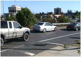
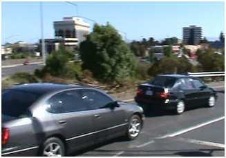
62 45 a b c d e Figure 3.3: (a) Motorcycle bypassing queue, (b) vehicle bypassing queue, (c) large truck entering on-ramp, (d) off-centered vehicles with respect to lane, and (e) adjacent vehicles simultaneously stopped on top of leading and trailing speed-trap sensors

63 Discussion Five queue estimation methodologies were studied using wireless magnetic sensors installed on a single lane loop on-ramp. Queue length estimation based on (i) occupancy measurements at ramp entrance, (ii) vehicle counts at on-ramp entrance and exit, (iii) speed measurements at ramp entrance, (iv) speed and flow-measurements and (v) vehicle re-identification were considered. The accuracy and reliability of the queue estimation methods were studied using ground truth data obtained from video. The occupancy-based queue estimation method may be used to determine if the ramp is either empty or full, but it cannot be used to estimate the vehicle queue length accurately. This approach is highly dependent on the time calculation interval over which occupancy is calculated, and under on-ramp saturated conditions may yield misleading results due to vehicle tendency to miss the sensor detection zone while at rest. Estimating queue length on the basis of counting on-ramp entering and exiting vehicles based on flow-measurements from wireless magnetic sensors, as it has been the case with loop detectors, is not an acceptable method because of its inability to correct for errors like detector miscounts and offsets resulting from initial conditions. The speed based queue estimation method appears to be capable of instantaneously determining the mode of the on-ramp queue: unsaturated, saturated, or in transition. Nevertheless, based on the results obtained in this study, this queue estimation approach is not suitable to accurately estimate queue lengths. The queue estimator based on flow-measurements and speed measurement appears to be suitable for ramp metering applications where accurate queue control is desired. This method seems better than the other four estimators studied, since it has consistent performance during uncongested and congested conditions, it can compensate from drifts in the queue estimate due to measurement errors, it is able to track the ground truth queue length closely, and even when significant estimation errors are observed, the estimate is able to recover fairly quickly. The vehicle re-identification based queue estimation method counts vehicles that enter and leave the on-ramp, while relying on vehicle re-identification information to prevent drifts in the queue estimate. This queue estimation method performed better than the other four methods during uncongested on-ramp conditions, but it was unable to accurately estimate queue lengths during saturated on-ramp conditions. One of the reasons was related to an increase in flow-measurement errors during on-ramp congested conditions. Another reason was the low vehicle matching rate observed at this site, which affects the ability of the method to correct for errors regularly, Finally, and most importantly, it is suspected that there was a large percentage of mismatched vehicles, which created the presence of abrupt large errors in the estimate. The unexpected poor results obtained with this method during congested conditions, and the potential of this method for accurate link vehicle-count, as predicted in [38], motivated the development of the modified vehicle re-identification algorithm presented in Chapter 4.

64 47 Chapter 4 Vehicle Re-Identification: Algorithm Revision, Modifications and Performance Analysis 4. Introduction The work presented in this chapter was motivated by the results obtained from the queue estimation field test performed at the Hegenberger Rd. loop on-ramp in the Caltrans Bay Area District and presented in Chapter 3. Five different queue estimation methods were studied, including one that is based on the vehicle re-identification algorithm described in detail in Section 2.3. The queue estimation method based on this vehicle re-identification algorithm was expected to be extremely accurate and reliable, as predicted on [28, 38]. As explained in Section 2.4, the link vehicle-count algorithm relies on a high percentage of correctly re-identified vehicles for accurate estimation results. At the Hegenberger on-ramp, this requirement was not met, since the number of re-identified vehicles was very low and inaccurate when vehicles were stoping and moving at low speeds as they were going over the detectors. For this reason, the vehicle re-identification based queue estimation method significantly under-performed in estimating queue lengths during congested on-ramp conditions. Vehicle re-identification by matching electromagnetic signatures captured from inductive or magnetic sensors appears as one of the most efficient and cost-effective methods to re-identify

65 48 vehicles without raising privacy concerns associated with vehicle tracking [34]. However, electromagnetic signature methods tend to be unreliable under congested conditions when stop and go traffic is present. Vehicle re-identification methods based on loop detectors, like the one described in [48], are not only sensitive to speed changes in between vehicle detection stations, but also to changes in velocity as the vehicles go over the detectors. Even when speed normalization is decoupled from the matching algorithm, as in [34], the algorithms still rely on the assumption that vehicles go over the detectors at constant speed. This assumption is unrealistic for implementations in arterial streets, congested freeways, and on-ramps where stop-and-go traffic is unavoidable. The vehicle re-identification method discussed in Section 2.3 does not rely on the constant speed assumption and does not require vehicle speed. However, the poor performance of this vehicle matching algorithm in the queue estimation study presented in Chapter 3 called for an algorithm revision, improvement and performance analysis. This chapter is organized as follows: The ground truth (GT) and vehicle detection system (VDS) data from the Hegenberger on-ramp used for this analysis is explained in Section 4.2. The revision details are presented in Section 4.3. Section 4.4 discusses the algorithm modifications. Section 4.5 contains the performance analysis of the original and modified vehicle re-identification method based on data from the Hegenberger on-ramp. Section 4.6 shows vehicle link-count estimation at two different locations, the Hegenberger on-ramp and a San Pablo Avenue segment in Albany, CA, using both versions of the vehicle re-identification algorithm. A discussion of the results is presented in Section Data Ground Truth Data Ground truth data was obtained from videos recorded on May, 2 from 4:7 p.m. to 5:35 p.m., the same videos used in Chapter 3. However, additional extraction of ground truth data from the videos was required for the research discussed in this chapter. The three independent cameras shown in Figure 3.5 were used to obtain the ground truth data. From the second camera (Figure 3.5 (b)) it was possible to obtain the time s GTk when each entering vehicle k crossed the entrance array, where s GT < s GT2 < s GTNGT. From the first camera (Figure 3.5 (a)) it was possible to get the time t GTl when each exiting vehicle l went through the exit array, where t GT < t GT2 < t GTMGT. The Hegenberger on-ramp ground truth data used in this chapter consists of two vectors {s GTk,k =,,N GT = 543} and {t GTl,l =,,M GT = 534} and the matching of upstream to downstream vehicles k l. The matching k l was done visually and resulted in 534 matches.

66 49 Vehicle Detection System Data Consider the link formed by the entrance and exit arrays shown in Figure 3.3. During the video recording time interval, detection events indexed i =,,N were registered by the entrance array at times s < s 2 < s N. Detection events indexed j =,,M were registered by the exit array at times t < t 2 < t M. The upstream sensor array measures a signature X i each time there is a vehicle detection event i and the corresponding time s i. The downstream sensor measures a signature Y j each time there is detection event j and the corresponding time t j. For this study, the vehicle detection system data consists of two arrays {(s i,x i ),i =,,N = 522} and {(t j,y j ), j =,,M = 527}. Note that due to the nature of the vehicle detection system, detection errors cannot be avoided and may create multiple signatures of the same vehicle at one location or may result on missing signatures due to undetected vehicles at the entrance and/or exit array as discussed in Chapter 3. To be able to determine the number of vehicles that are correctly matched by the algorithm and the percentage of those vehicles that are mismatched, mappings of the form k i and k l j were obtained. With these it is possible to determine if a signature pair (X i,y j ) corresponds to the same vehicle or to different vehicles. Vehicle Subsets During the video recording period, the traffic modes that arise inside the ramp are classified into two: uncongested and congested. For this analysis, uncongested conditions correspond to the time interval from 4:7 pm to 5:7 pm, when the on-ramp queue was below on-ramp capacity and vehicles with index k for k 399 went through the on-ramp. The uncongested vehicle subset is constituted by these vehicles. The congested conditions time interval occurs from 5:7 pm to 5:35 pm, when the queue length was around or beyond on-ramp capacity, vehicles were stopping or going slowly over the entrance array, and vehicles with entering vehicle index k for 4 k 534 went through the ramp. The congested vehicle subset is composed of these vehicles. Based on the vehicle detection system data, it is possible to achieve a maximum correct matching of 477 vehicles assuming a perfect matching algorithm, where 362 vehicles correspond to the uncongested vehicle subset and 5 to the congested one. 23 Chosen Vehicles In order to be able to analyze the vehicle re-identification algorithm in detail, 23 vehicles were chosen from the 543 that entered the ramp, as shown in Table 4.. The selection criteria was that their entrance and exiting signatures were available and unique and that they were traveling through the middle of the lane when going over the arrays.

67 5 4.3 Vehicle Re-Identification Method Revision Signal Processing Step Revision The plots on Figure 4. are gray scale coding of the distance matrix of the 23 chosen vehicles signatures (left) and the distance matrix of the complete vehicle signatures data set (right) calculated using the original signal processing algorithm. As explained in Section 2.3, each square in the plots represents a distance between a X i and Y j vehicle signature combination; a darker color indicates shorter distance and a greater chance that X i and Y j come from the same vehicle. The gray scale used in Figure 4. and Figure 4.3 goes from min(d) to.75 median(d), where D represents the distance matrix being plotted. Figure 4. (left) shows multiple dark squares along the diagonal, where diagonal entries correspond to distances between signatures of the same vehicle. The distance value of the diagonal entries are listed in Table 4.. Note that the diagonal entries corresponding to the congested vehicle subset are not as dark (i.e., small) as the uncongested ones. It seems that phenomena occurring specifically during congestion affect the f and g probability density functions (pdf). This is further corroborated by the plot of the distance matrix for the complete data set, shown on Figure 4. (right). For the uncongested vehicle subset, a diagonal line is present and is consistently darker and visually distinguishable from the off-diagonal D entries. However, dark diagonal entries vanish at the lower right portion of the plot, where the distances between vehicle signatures from the congested vehicle subset are plotted. The original signal processing algorithm produces different f and g pdfs for different on-ramp modes. The f and g pdfs become similar during on-ramp congested conditions, which reduces the Uncongested Conditions Congested Conditions Index Vehicle Org. Mod. Index Vehicle Org. Mod. k Type Dist. Dist. k Type Dist. Dist. 76 minivan car truck SUV truck pickup pickup car truck SUV car car minivan car SUV car pickup car car car car SUV van Table 4.: 23 chosen vehicles

68 5 Distance between Vehicle Signatures (23 Chosen Vehicles) Distance between Vehicle Signatures (Complete Data Set) Entering Vehicle Signatures Entering Vehicle Signatures Exiting Vehicle Signatures Exiting Vehicle Signatures Figure 4.: Original distance matrix for the (left) 23 chosen vehicles (right) complete vehicle data set effectiveness of the matching algorithm. The signal processing method should be able to maintain the f and g pdfs invariant to traffic conditions. Vehicle Signatures Revision Entrance and exit signatures of the 23 chosen vehicles were studied in order to explain the different f and g pdfs observed for the uncongested and congested vehicle subsets. Figure 4.2 (b) shows two slices of the entrance and exit signatures of vehicle k = 527. Note that the upstream slices show more peaks than the downstream ones. Vehicle 527 went slowly over the entrance array and at free flow speed over the exit array. The extra peak phenomenon was observed in the signatures of vehicles going slowly or stopping over the entrance arrays. During congestion, vehicle signatures tend to have more noisy peaks, most of which are small compared to the dominant peaks of the signatures. A vehicle signature with noisy peaks leads to a larger µ f and σ f, since the difference on the number of peaks is penalized in the distance calculation independently of their magnitude. Another finding was related to the importance of the x, y and z components of a vehicle signature slice when calculating distances. The original method assigned the same weight to the distances obtained between the x, y, and z components. By changing these weights, it was observed that it is possible to increase the dissimilarity between the f and g pdfs during congestion. Sometimes signature slice components (x,y and z) of different vehicles look very similar after

69 52 (a) (b) (c) x x x y x x Entrance Array z x x x.3.35 y z x x x x x x x x x Exit Array Figure 4.2: Vehicle k = 527 two signature slices at the entrance and exit arrays (a) raw peak values, (b) processed for original distance calculation (c) processed for modified distance calculation the peak sequences have been normalized by the maximum absolute value of their elements as a preprocessing step before the distance calculation is performed. The distance between such slices is small and may lead to significant errors in the matching step. It was observed that when the raw amplitude of the peaks is considered in the distance calculation between such signatures, the distance increases for signatures from different vehicles and remains unchanged for signatures from the same vehicle. Matching Step Revision The matching algorithm was studied using the 23 chosen vehicles. It was concluded that the matching rate and its accuracy are directly related to µ f, σ f, µ g, σ g and β. Furthermore, it was

70 53 Default f and g 23 vehicles f and g Iterative f and g Both Original Modified Original Modified µ f σ f µ g σ g Table 4.2: Different f and g statistics for the original and modified signal processing methods observed that one of the reasons that explain the low matching rate during the queue estimation study presented in Chapter 3, even during uncongested on-ramp conditions, was related to the f and g parameters used at the Hegenberger on-ramp. The f and g statistics used at the ramp where assumed to be equal to the ones satisfactorily used at many arterial installation sites (see Table 7.2, second column). This assumption was incorrect, since f and g statistics based on the 23 chosen vehicles distance matrix (see Table 7.2), show that the default f and g statistics do not accurately model signature distances at the on-ramp. It is important to calculate f and g parameters for each test site, since they are site dependent and influence the matching rate. These parameters can be obtained using an iterative method as the one suggested in [28], which does not require ground truth data. Note that the iteratively obtained f and g parameters extracted from the complete vehicle data set are very similar to the ones extracted from the 23 chosen vehicles for both the original and the modified signal processing methods, and very different from the default values, as seen in Table Vehicle Re-Identification Method Modifications Signal Processing Algorithm Modification The following modifications were implemented in the original signal processing algorithm: i) There were adjustments in the way vectors of different sizes are compared using dynamic time warping. This included modifying the way in which extra peaks are penalized when vectors being compared are of different sizes. ii) A peak processing step was implemented before the distance calculation in order to remove noisy peaks resulting from vehicles traveling slowly or stopping on top of the arrays. This step uses the local time stamp component available for each signature peak described in Section 2.3. See Figure 4.2 for a comparison between the preprocessed signature slices and the processed signature slices using the original and the modified methods. iii) Different weights were assigned to the x, y and z components of the distance between two vehicle slices. The x component was assigned the larger weight and the y component the smaller one. iv) The distance calculation is performed without normalizing the peak sequences. Once a distance is

71 54 obtained between the components of two signature slices, a normalization step is performed. Signal Processing Improvements The plot on Figure 4.3 (left) is a gray scale coding of the distance matrix of the 23 chosen vehicles signatures using the modified signal processing algorithm. Note that in contrast to Figure 4. (left), dark squares are present along the entire diagonal, thus suggesting that f and g statistics are somehow invariant to on-ramp traffic conditions. In Figure 4.3 (right), where the distance matrix of the complete data set calculated using the modified distance method is plotted, it is possible to see a darker diagonal band at the bottom right corner of the plot. This diagonal band corresponds to distances from signatures generated by the same vehicle in the congested vehicle subset. This distinction between diagonal and off-diagonal entries was not present in the original distance matrix shown in Figure 4. (right), which helps explain why the matching rate was specially low and inaccurate during congestion. From Table 4. it is possible to see that the modified distance among signatures from the same vehicle are similar for the uncongested and congested vehicle subsets. Figure 4.4 shows for each of the 23 chosen vehicles, k, D k = {d(k,l) = δ(x k,y l ) l 23}. For each D k, the data points given by δ(x k,y l ) for l k are plotted as black dots while δ(x k,y k ) is plotted as a blue circle. Figure 4.4 (top) contains the distances obtained using the original method. This plot shows that for vehicles from the congested vehicle set, δ(x k,y k ) is generally not the smallest entry of D k, Distance between Vehicle Signatures (23 Chosen Vehicles) Distance between Vehicle Signatures (Complete Data Set) Entering Vehicle Signatures Entering Vehicle Signatures Exiting Vehicle Signatures Exiting Vehicle Signatures Figure 4.3: Modified distance matrix for the (left) 23 chosen vehicles (right) complete vehicle data set

72 55 ORIGINAL Distance between Vehicle Signatures.8 Distance k th Vehicle MODIFIED Distance between Vehicle Signatures.8 Distance k th Vehicle Distance between k th entrance vehicle signature and all exit vehicle signatures except the k th Distance between the k th entrance vehicle signature and the k th exit vehicle signature Figure 4.4: Comparison between the (top) original and the (bottom) modified distance method which is undesired and degrades the performance of the matching algorithm. With the modified signal processing method, as displayed in Figure 4.4 (bottom), δ(x k,y k ) tend to be the lowest element of D k by a clear margin, for vehicles belonging to the uncongested and congested subsets. This increases the matching rate and its accuracy. Matching Algorithm Modification The matching algorithm was not modified. However, it was observed that the f and g statistics as well as β play an important role in the number of matched vehicles and the percentage of mismatched vehicles produced by the algorithm. These findings were part of the motivation behind the work presented in Chapter 7, where a tuning system was developed in order to facilitate setting these parameters for any vehicle re-identification system installation.

73 Vehicle Re-Identification Results Default vs Iterative µ f, σ f, µ g, σ g Results In this section, two different sets of µ f, σ f, µ g, σ g were used to study the effect of f and g pdfs variations on the matching algorithm performance for the original and the modified methods. The default and the iteratively obtained set of parameters, listed in Table 7.2, were used. Table 4.3 shows the results obtained with the matching algorithm for the complete vehicle data set, the uncongested vehicle subset and the congested vehicle subset. The modified method has a higher number of re-identified vehicles in comparison to the original method for both sets of parameters. The number of matches over the original method results increased by 56% for the default f and g and by 3 % for the iterative ones. For the original method 23 % of vehicles were incorrectly matched when using the default parameters and 6 % when using the iterative parameters. For the modified method, for the default and iterative f and g, the overall percentage of mismatched vehicles remained the same, 7%. The modified distance method seems to increase the matching rate in comparison with the original distance method while keeping the percentage of incorrect matches low and constant for significant µ f, σ f, µ g, σ g variations. Furthermore, the use of f and g statistics that properly model the distance between signatures (e.g., iteratively obtained parameters), makes a significant difference in the matching rate without degrading accuracy. When the results of the matching algorithm are analyzed by vehicle subset, further differences are observed. First, the percentage of mismatched vehicles is larger for the congested vehicle subset in comparison to the uncongested one, for both methods. The percentage of incorrectly matched vehicles changes from 6% for the uncongested subset to 62.5% for the congested one when using the original method with default f and g parameters. The percentage of mismatched vehicles changes from 2% to 3% when the iterative f and g parameters are used instead. The modified distance method also shows differences in the accuracy obtained for the uncongested and congested vehicle subset results. The percentage of incorrect matches changes from 6% to % when using default f and g parameters. This number changes from 5% for the uncongested Default f and g Iterative f and g Original Modified Original Modified Matched (complete data set) incorrectly matched Matched (uncongested subset) incorrectly matched Matched (congested subset) incorrectly matched 3 2 Table 4.3: Matching results using the default and iterative f and g from Table 7.2 for the original and modified method

74 57 Matching Algorithm Results as a Funtion of Probability of Turn (β) % of Mismatched Veh (Uncong) % of Mismatched Veh (Cong) Original: Total Matches (out of 477) Original: Uncongested Matches (out of 362) Original: Congested Matches (out of 5) Modified: Total Matches (out of 477) Modified: Uncongested Matches (out of 362) Modified: Congested Matches (out of 5) 6 5 Original Method Modified Method 6 5 Original Method Modified Method Number of Vehicles % 4 3 % Probability of Turn (β) Probability of Turn (β) Probability of Turn (β) Figure 4.5: (left) Matched vehicles as a function of β, (middle) % of uncongested mismatched vehicles as a function of β and (right) % of congested mismatched vehicles as a function of β subset to % for the congested one when using the iterative f and g parameters. The decrease in performance of the matching algorithm during congestion is observed for both the original and the modified vehicle re-identification method. However, the original method accuracy is highly dependent on the values of µ f, σ f, µ g, σ g while the accuracy of the modified method seems to remain unchanged. Iterative µ f, σ f, µ g, σ g with varying β Results The matching algorithm results presented in this section were obtained using the iteratively obtained µ f, σ f, µ g, σ g parameters and using both the original and the modified vehicle re-identification method as β was varied. From Figure 4.5 (left) it is observed that the modified method has higher matching rate for all β values considered for this analysis for the complete vehicle data set, the uncongested vehicle subset and the congested vehicle subset. Figure 4.5 (middle) shows the percentage of incorrectly matched vehicles for the uncongested vehicle subset as function of β. Note that both methods have a mismatch percentage that remains somehow constant as β is varied. However, an advantage of the modified distance method is that the percentage of incorrect matches is around or below 8%, in comparison to the 5% obtained with the original method. Figure 4.5 (right) shows the percentage of incorrectly matched vehicles for the congested vehicle subset. The percentage of incorrect matches are larger for all β for the original and modified method in comparison to the uncongested

75 58 results. Observe that while the original method mismatch percentage increases from 2% at low β values to 6% for large ones, the modified method percentage of incorrectly matched vehicles remains around or below 4% for all β values. The original algorithm matching rate and accuracy is affected by β variations. The modified distance method matching rate is affected by changes in β, but the accuracy of the matches seems to remain constant. 4.6 Application: Link Vehicle-Count based on Vehicle Re-Identification In this section, link vehicle-count estimation results for the Hegenberger on-ramp and a San Pablo Avenue segment in Albany, CA, are presented. For the Hegenberger on-ramp analysis, the main goal is to show that the modified method improves link vehicle-count estimation performance, especially for saturated conditions. In the first part of the Hegenberger analysis, the same data set presented in Chapter 3 is used to show improvement on the queue estimate. In the second part, the analysis is based on queue estimation results using the modified method on data from March 2 to March 27, 2. With these data sets it is possible to comment on the consistency and reliability of the estimated queue profiles by comparing them with profiles that are expected under different circumstances (e.g., morning vs afternoon, weekday vs weekend, ramp metering vs no ramp metering), as well as by comparing them with queue estimates based on the speed and flow-measurements method discussed in Chapter 3. In the second part of this section, a study of arterial link vehicle-count estimation using the original and the modified method is presented. The analysis is done with vehicle detection data from a San Pablo Avenue segment that has been used in previous studies, [28, 27], and for which the original vehicle re-identification system showed a high matching rate and good accuracy, but where stop-and-go traffic around the sensor arrays was uncommon. Improved On-ramp Queue Estimation Queue Estimation for May, 2 With the modified vehicle re-identification algorithm and with f and g parameters that correspond to the distance matrices calculated at the Hegenberger installation, the vehicle matching rate and accuracy during saturated ramp conditions was improved, resulting in a more accurate and reliable queue estimate.

76 59 Figure 4.6 (top) shows the queue estimation results presented in Chapter 3 using the original method with information about instances when vehicles were re-identified and additional information showing which of those matches were incorrect (marked with red circles). For the time interval corresponding to the plot, the matching rate, out of the maximum possible based on the recorded signatures, was 22 %, i.e., 7 out of 477, and from these matched vehicles, 25 % were incorrectly matched. There were 26 mismatched vehicles, 2 of which were mismatched during the congested time interval, when only 35 out of the 534 vehicles that were studied during the complete analysis went through the on-ramp. It is clear that one of the reasons that explains the poor performance of the queue estimation method was a considerably large percentage of mismatched vehicles during congestion. Figure 4.6 (middle) shows the queue estimation results for the same data used in Chapter 3 using the original method and f and g parameters that correspond to the installation at the Hegenberger on-ramp. Again, the plot shows the ground truth and estimated queue lengths with information about instances when vehicles were re-identified and additional information showing which of those matches were incorrect (marked with red circles). With the new f and g parameters, the matching rate increased to 58 %, i.e., 276 out of 477 vehicles, and from these matched vehicles, 5 % were incorrectly matched. There were 42 mismatched vehicles, 8 of which were mismatched during the congested time interval. During uncongested conditions, the queue estimate improved, especially during the time interval [6.3 h, 6.4 h], as a result of the higher matching rate and smaller percentage of mismatched vehicles. During congestion, the queue estimate improved, but it was still inaccurate and with significant errors that are unacceptable for accurate queue control applications. This poor performance during congested conditions, as before, is closely related to the large percentage of mismatched vehicles. Figure 4.6 (bottom) shows the queue estimation results for the same data used in Chapter 3 using the modified method and f and g parameters that correspond to the installation at the Hegenberger on-ramp, and that were also used in Figure 4.6 (middle). Figure 4.6 (bottom) shows the ground truth and estimated queue lengths with information about instances when vehicles were reidentified and additional information showing which of those matches were incorrect (marked with red circles). The matching rate, using the modified method and the adjusted parameters, increased to 7 %, i.e., 332 out of 477 vehicles, and from these matched vehicles, 7 % were incorrectly matched. There were 23 mismatched vehicles, 9 of which were mismatched during the congested time interval. During uncongested conditions, the queue estimate improved over the two previous cases due to a higher matching rate and smaller percentage of mismatched vehicles. During congestion, the queue estimation error is larger in comparison to the uncongested case, but with the modified vehicle re-identification algorithm, the error remains bounded and the queue estimate is able to track the ground truth queue length with sufficient accuracy for accurate queue control applications. Mismatched vehicles cannot be completely avoided, but since now they represent a small percentage of the matched vehicles, they do not introduce significant errors in the queue estimate. However, there are time instances when there are no mismatched vehicles, e.g., [7.23 h, 7.35 h], and still, queue estimation errors are observed. These errors are due to an increase in flow-measurement inaccuracies during on-ramp congested conditions. Nevertheless, a higher

77 6 Queue Length [Veh] Queue Length [Veh] Queue Length [Veh] Queue Length (ground truth data) Queue Length (veh re id data) Matched Vehicles (7/477) Mismatched Vehicles (26/7) Queue Length Based on Vehicle Re Id vs Time of Day, May, Queue Length (ground truth data) Queue Length (veh re id data) Matched Vehicles (276/477) Mismatched Vehicles (42/276) Queue Length (ground truth data) Queue Length (veh re id data) Matched Vehicles (332/477) Mismatched Vehicles (23/332) Time of Day [hour] Figure 4.6: Hegenberger on-ramp queue length estimates using β =.5 with (top) the original method and default f and g, (middle) original method and Hegenberger f and g and (bottom) modified method and Hegenberger f and g. matching rate allows for a better and rapid correction of these errors when they occur. Queue Estimation from March 2 to March 27, 2 For the following analysis, ground truth data from video are not available to study the performance of the vehicle re-identification algorithm or the queue estimation results. However, there are multiple sources of information that can be used to infer what would be reasonable results. First, note that from the vehicle re-identification algorithm, it is possible to calculate the travel time of vehicles going through the on-ramp, as explained in Section 2.4. With the travel time, it is possible to check if there are any major problems with the vehicle re-identification algorithm results. Travel times should not be smaller than zero, and, unless a major accident occurs on the freeway and blocks the on-ramp, should not be larger than 8 minutes, calculated based on the minimum allowed metering rate and the Hegenberger on-ramp capacity. If travel times happen to be consistently outside this range, then that would indicate a very bad vehicle re-identification performance. Second, queue estimates should not be less than zero or greater than 25 vehicles. Furthermore, it is expected that during weekdays there should be an increase in the queue length and/or travel time during the morning peak traffic time, i.e., 6 a.m. to 9 a.m., and the afternoon traffic time, i.e., 3 p.m. to 7 p.m., because during those times ramp metering is active and demand tends to be higher. On weekends, ramp metering is not active, and demand is usually low unless a special event takes place, e.g., event at the Oracle Arena or Oakland Coliseum located next to the

78 6 Hegenberger on-ramp. All these indirect sources of information about what can be expected at the on-ramp in terms of travel time and queue lengths were used to comment on the reliability of the vehicle re-identification and queue and travel time estimation results using the modified method for one week. Additionally, in order to further study the performance of queue estimation based on the modified method, the data for two time intervals during this week were used. For both times, the queue estimation method based on speed and flow-measurements discussed in Chapter 3 was used for comparison and validation purposes. Figure 4.7: Hegenberger on-ramp (top) queue estimates and (bottom) travel time estimates from Monday, March 2, to Sunday, March 27, 2 Figure 4.7 shows the queue length and travel time estimates from 2 a.m. ( h) Monday, March 2, 2, to :59 p.m. (23.9 h) Sunday, March 27, 2. In the figure it is possible to observe differences between the estimates generated during weekdays from those obtained based on weekend data. For standard weekdays in the Hegenberger on-ramp, the queue length reaches values of around 22 vehicles, and travel times of up to 3 seconds. During standard weekend days, a different pattern is observed. Queue lengths tend to be smaller, reaching usually around vehicles, and travel times generally do not exceed seconds. For the week under study, March 2 to March 25 correspond to standard weekdays, March 27 corresponds to a standard weekend day, and March 26 corresponds to a non-standard weekend day that resulted from a game at the

79 62 Oakland Coliseum. Queue Length Estimates vs Time of Day, March 22, 2 25 Queue Length (veh re id data) Matched Vehicles (884 matches/72 entering veh) Queue Length (arrays + speed trap data, [ Inf, Inf]) 2 Queue Length [Veh] Time of Day [hour] Figure 4.8: Queue estimates at the Hegenberger on-ramp on Tuesday, March 22, 2, from 5.25 h to 8.25 h Figure 4.7 (top) shows the queue length estimates for the complete week under analysis. In the queue estimates from March 2 to March 25 it is possible to observe a time interval for which the queue lengths are higher than during the rest of the day. This time period corresponds to the afternoon peak hour, when ramp metering is activated, demand is higher than during the rest of the day, and vehicle queues that extend around or beyond the entrance of the on-ramp are frequently formed. During weekdays, ramp metering is also active during the morning peak hour. However, the queue estimate profiles for these days do not suggest that ramp metering is active and that longer queues are forming during the morning. This is expected because at the Hegenberger onramp, demand is not high during the morning peak hour in comparison to the afternoon rush hour. Nevertheless, even when the vehicle queues do not reach values larger than 5 vehicles, it is possible to observe that during a standard weekday morning with short queues, drivers going through the on-ramp experience a larger delay as a result of active ramp metering, as observed in Figure 4.7 (bottom) at the early hours of each weekday. The maximum travel time observed for the different weekdays vary from day to day. This is the result of the traffic responsive ramp metering controller used at the ramp, which tends to increase the waiting time of vehicles in the queue if mainline traffic conditions in the vicinity of the on-ramp degrade. For this particular week, the largest travel times are observed during March 23 and March 24, which according to PeMS data [4], were the two weekdays with the worst mainline conditions around the Hegenberger on-ramp. Figure 4.8 plots two vehicle queue profiles, one estimated with the method based on the modi-

80 63 fied vehicle re-identification algorithm and the other with the method based on vehicle counts and speed, for Tuesday, March 22, from 5.25 h to 8.25 h. This is a time interval during the afternoon rush hour when the on-ramp was expected to have congested and uncongested periods as the result of ramp metering and oscillations in demand. It is important to emphasize that both estimates could take negative values or be larger than on-ramp capacity. From the figure it is clear that both queue estimates follow each other closely, but as in Chapter 3, the queue estimate using speed and flow-measurements tends to slightly overestimate the queue. Both queue profiles are consistent for the complete time interval and for the most part are within a reasonable range, i.e., [,25], which suggest that both estimates are likely to be close to the real queue length. Furthermore, the matching rate over the time interval shown in the plot is 75 %, i.e. 882 out of 72 vehicles that entered the on-ramp were re-identified, which is better than the matching rate from the previous section, and further increases the confidence on both estimates Queue Length Estimates vs Time of Day, March 26, 2 Queue Length (veh re id data) Matched Vehicles (88 matches/32 entering veh) Queue Length (arrays + speed trap data, [ Inf,Inf]) Queue Length [Veh] Time of Day [hour] Figure 4.9: Queue estimates at the Hegenberger on-ramp on Saturday, March 26, 2, from 6.5 h to 7.83 h Figure 4.7 shows queue length and travel time estimates for March 26 2, a non-standard weekend day. For this day it is possible to observe a time interval in the afternoon for which the estimates are significantly larger. On March 26 there was a soccer game at the Oakland Coliseum that ended at around 6 h, and that induced a large demand at the on-ramp because people exiting the stadium were trying to get into the freeway. Since the demand was high and constant and ramp metering was not activated, the queue length was not oscillating between uncongested and congested modes, as it was the case for the afternoon on March 22. Even when the number of vehicles at the on-ramp was around capacity from around 6.5 h to 7.8 h, as observed in Figure 4.9, the travel time experienced by the drivers during this time was less than seconds, significantly

81 64 less than the travel time observed during an average weekday rush hour when vehicle queues had similar lengths and ramp metering was active. This scenario clearly illustrates that knowing travel time information besides queue length allows for a better understanding of driving conditions at the on-ramp in comparison to just knowing queue lengths. Figure 4.9 plots two vehicle queue profiles, one estimated with the method based on the modified vehicle re-identification algorithm and the other one with the method based on vehicle counts and speed, for Saturday, March 26, from 6.5 h to 7.83 h. Both estimates are unconstrained and can take any value on the interval [-Inf, Inf]. During this period, the on-ramp transitioned to congested conditions at the beginning of the interval, stayed in a congested state for more than an hour, and then it transitioned back to an uncongested state. The two estimates on the figure have a similar shape, but the one using speed and flow-measurements significantly overestimate the length of the queue. This degradation in performance may be due to driving behavior and queue dynamics changes as the result of inactive ramp metering, which makes Eq. (3.) less reliable. The queue profile based on vehicle re-identification is reasonable and consistent with what it is expected at the on-ramp right after an event at the coliseum, i.e., a saturated ramp for an extended period right after the end of the event due to a high constant demand and a queue estimate within [,25]. Furthermore, these queue estimates are based on a 67 % matching rate, i.e. 88 out of 32 vehicles that entered the on-ramp were re-identified, which is an acceptable matching rate for accurate queue estimation, as discussed in Section 2.4. In this section we presented the queue length and travel time estimates calculated using the modified vehicle re-identification system for one week in March 2. We showed how queue lengths and travel times vary as a function of the day of the week (i.e. weekday vs. weekend), due to events taking place around the Hegenberger on-ramp (e.g., games at the Oakland Coliseum) and as a function of ramp metering. The results using the modified method were reasonable, consistent with the analysis documented in Chapter 3, and showed that queue length information may not be sufficient to evaluate traffic conditions and that by knowing travel time in addition to queue length, it is possible to get a much better assessment of the driving conditions at the on-ramp. Arterial Link Vehicle-Count Estimation: Original vs Modified Method Arterial Test Site The San Pablo Avenue arterial link used for this analysis is a.24 km (.5 mile)-long segment that intersects Washington Avenue and Solano Avenue in Albany, CA (see Figure 4.). Even though the San Pablo avenue is a two-way street, the data presented in this section correspond to the fast lane of the southbound direction, where two five sensor arrays were installed as shown in Figure 4.. This test site has been used for analysis related to arterial travel time estimation based on the original vehicle re-identification system [28, 27, 4]. This site is a suitable location to study the performance of an arterial link vehicle-count estima-

82 65 (a) San Pablo Ave Sensor Array (b) Washington Ave Solano Ave San Pablo Ave START Sensor Array Fast Lane Slow Lane END Figure 4.:.5-mile segment of San Pablo Avenue in Berkeley, CA: (a) aerial view with long queues and (b) segment schematic tor, since it has a configuration and driving dynamics that encompasses what can be encountered in many arterial streets where traffic-responsive intersection control is desired: drivers can go into or out of the link at any location along the segment, as the result of lane changing, and large number of vehicles get in and out of the link not only at the start and end locations, but also at the intersections in between. Furthermore, queue formation is common in this link as the result of the traffic light at intersection between San Pablo Avenue and Solano Avenue, as observed in Figure 4. (a). The locations of the sensor arrays at this site follow the manufacturers guidelines, i.e., the arrays were installed downstream of intersections to maximize the chances of vehicles going at free flow speed as they travel over the sensor arrays.

83 66 Ground Truth Data For this analysis, it was possible to obtain ground truth data from a video recorded from 2:43 p.m. (4.7 h) to 3:43 p.m. (5.7 h) on Thursday, October 3, 28. A camera was placed at a height and orientation that captured in a single shot, the complete link formed by the two arrays. This video was previously used for an experimental analysis of the original vehicle re-identification algorithm and travel time estimator in [27]. The ground truth data was useful in this section to compare vehicle re-identification results between the original and the modified algorithms. However, in order to analyze the performance of link vehicle-count estimation results, it was necessary to extract additional information from the video. Ground truth link vehicle-count data was recorded by stopping the recording every 5 seconds, and counting the number of vehicles in the fast lane in between the two sensor arrays. The link vehicle count ground truth data is plotted in Figure 4.. Results This section is divided into two parts. In the first part, vehicle re-identification results based on the original and the modified method are presented and compared among each other and to ground truth data. In the second part of this section, link vehicle-count estimates based on both re-identification methods are compared to ground truth data. The following discussion is based on data from Table 4.4. For the time interval from 4.7 h to 5.7 h on October 3, 28, 539 vehicles were observed to go over the start (upstream) array and 473 vehicles were observed to go over the end (downstream) array. The vehicle detection system during the same time interval recorded 524 vehicles at the upstream location and 424 vehicles at the downstream location. As in the Hegenberger on-ramp, there are flow-measurement errors, with an overall 3% counting error at the upstream location and % error at the downstream location. 349 vehicles, out of the 539 vehicles that went over the upstream array, exited the link going over the downstream array. Out of the 349 vehicles, the original method re-identified 84 %, with 4 % of them incorrectly matched. On the other hand, the modified method re-identified 83 % of the vehicles, with a 6 % mismatch. Based on these results, it seems that the modified method does not offer any improvement in performance when free flow traffic conditions are present in the vicinity of the sensor arrays, as it was the case at this site. Furthermore, the original and the modified methods seem to have comparable performance under such conditions. The link vehicle-count estimates for this analysis were calculated every time a vehicle exiting the arterial segment at the downstream location was re-identified. For this reason, Eq. (2.8) was used instead of Eq. (2.9), used for queue estimation at the Hegenberger on-ramp. An important difference between both analyses relies on the granularity of the ground truth data. For the Hegenberger analysis, ground truth data for link vehicle-count was updated every time a vehicle entered or left the on-ramp. On the other hand, for this analysis, link vehicle-count ground truth data is not as detailed and is only updated every 5-s. By reducing the frequency at which link vehicle-counts are estimated by using Eq. (2.8) instead of Eq. (2.9), it is easier to compare the results.

84 67 Ground Original Modified Truth Method Method Start Array End Array Start Array End Array Start Array End Array Vehicle Count Matches Incorrect Matches - 7 Table 4.4: Ground truth and matching results using µ f =.8, σ f =.7, µ g =.6, σ g =.2 and β =.5 At the San Pablo segment, it is not possible to measure n out, the number of vehicles that go over the upstream array but exit the link before reaching the downstream array, or n in, the number of vehicles that entered the link without going over the upstream array and exited it going over the downstream array. To overcome this limitation, n net = n out n in is taken into account by using η, a correcting factor applied to the link vehicle-count estimated under the assumption that n net =, as explained in detail in Section 2.4. For this analysis, η =.5, which was chosen based on the data from Table 4.4. Figure 4. (top) shows the link vehicle-count ground truth data and the estimate based on the original vehicle re-identification method from 4.7 h to 5.7 h on October 3, 28. In the plot, the estimate is updated only when a vehicle is re-identified, marked with a blue dot. A red circle around a blue dot indicates that at that particular instance, the re-identification is incorrect. From the plot, it is clear that the estimate follows the ground truth data closely. Note that even when mismatched vehicles are observed, the estimation errors remain small. Figure 4. (bottom) shows the same type of plot, but showing estimation results based on the modified method. Even though the mismatched vehicles are different for both methods, the performance is similar, and the estimate closely tracks the ground truth link vehicle-count. Figure 4. further corroborates that both methods have comparable performance when stop-and-go traffic is not present in the vicinity of the arrays. Additionally, it shows that accurate and reliable link vehicle-count can be achieved on arterial links using the estimation method based on vehicle re-identification, and discussed in Section Discussion The vehicle re-identification method based on matching vehicle magnetic signatures obtained with wireless magnetic sensors was studied in detail using data from the Hegenberger single lane onramp. Based on this study, different modifications were implemented in the algorithm in order to address limitations of the system when vehicles travel slowly or stop while going over the detectors. The original and modified vehicle re-identification algorithm results were compared against ground truth data obtained from video. Based on the ground truth data it was possible to determine the

85 68 Link Vehicle Count [Veh] Link Vehicle Count [Veh] Link Vehicle Count vs Time of Day, Thursday October 3, 28 Link Vehicle Count(ground truth, 5 s interval) Link Vehicle Count (veh re id Original method) Matched Vehicles (293/349) Mismatched Vehicles (/293) Link Vehicle Count(ground truth, 5 s interval) Link Vehicle Count (veh re id Modified method) Matched Vehicles (289/349) Mismatched Vehicles (7/289) Time of Day [hour] Figure 4.: Link vehicle-count estimates using vehicle re-identification with (top) the original method and (bottom) the modified method percentage of vehicles that were re-identified and the number of vehicles that were misidentified as a function of different algorithm parameters. The modified distance method resulted in an increase in the number of re-identified vehicles over the original system while keeping an overall incorrectly matched vehicle percentage below % when matching algorithm parameters like µ f, σ f, µ g, σ g, and β were varied. The best performance was observed during uncongested on-ramp conditions, with a percentage of mismatched vehicles around or below 8%, while during congested on-ramp conditions this number increased to 4%. In this Chapter, it was also possible to quantify how an improved vehicle re-identification algorithm directly impacts link vehicle-count estimates. Using the original and the modified vehicle re-identification systems, the queue length at the Hegenberger on-ramp for the same time interval used for the analysis presented in Chapter 3 was re-evaluated. The queue estimation accuracy improved significantly with the modified method, as the result of a higher matching rate and the decrease in the percentage of mismatched vehicles, especially during congested conditions. Furthermore, by using one week of data from March 2 to March 27, 2, it was possible to show that with the modified vehicle re-identification method, queue estimates are consistent with what is expected in the field. Finally, the queue estimation based on the modified vehicle re-identification method and the queue estimation based on speed and flow-measurements were compared for two time intervals, one that corresponded to a common queue profile during peak traffic while the other corresponded to a queue profile resulting from a special event. Based on these comparisons, the modified vehicle re-identification method seemed to be better at estimating the queue, in particular,

86 69 during the special event time period. Finally, by using the vehicle re-identification method for arterial link vehicle-count estimation on the San Pablo Avenue site, it was possible to show two things: i) the original and the modified vehicle re-identification algorithms yield comparable results when stop-and-go traffic is not present as vehicles go over the sensor arrays, and ii) the link vehicle-count presented in Section 2.4 is an accurate and reliable estimator that can be used for real-time intersection traffic control applications that require arterial link density.

87 7 Chapter 5 Arterial Travel Time Estimation based on Vehicle Re-Identification: Performance Analysis 5. Introduction The research presented in this chapter is a continuation of the work presented in Chapter 4, where the vehicle re-identification algorithm used in the arterial travel time estimation system discussed in Section 2.4 and considered for this analysis, was revised, improved and validated at a single lane loop on-ramp and at a short arterial segment. The resulting modified method showed an improved vehicle re-identification matching rate and accuracy at the on-ramp, where stop-and-go traffic in the vicinity of the upstream sensor array was common. The original vehicle re-identification method has been used and evaluated at multiple sites, where the vehicle detection systems were usually installed following the manufacturer recommendations to avoid stop-and-go traffic around the sensor arrays. A detailed study is presented in [43], where travel time estimation based on the original vehicle re-identification system was evaluated along the Pendleton Pike corridor in Indianapolis, IN, using six arterial segments, each approximately mile long, for 3 hours during the afternoon peak traffic time. These segments had a 4/45 mph speed limits, and there were at least two signalized intersections in each of them. The reported percentage of matched vehicles out of the entering lane volume for each of the segments was in the range [38%, 48%]. This range may seem low, but note that the matching rates in this analysis were

88 7 not calculated based on the number of vehicles that went through the links but on the volume at the upstream locations, i.e., lane changing and inflow and outflow of vehicles at the intersections were not taken into account. The analysis reports the accuracy of the matched vehicles using ground truth data from video. Based on the camera system in place, it was possible to confirm that on average, at least 9% of the matched vehicles were correctly re-identified (sometimes confirmation was not possible due to visual occlusions). This study concluded that the system performance was accurate and reliable for the segments under consideration and that the matching rates were large in comparison to other probe vehicle data collection methods. Detailed studies of the original vehicle re-identification system at heavily congested arterial streets are not available. Since performance analyses based on ground truth data are time consuming and expensive, it is usually assumed that the system performance at such locations should be comparable to those reported in studies like [27, 43]. However, after observing how different vehicle re-identification results can arise as the result of stop-and-go traffic in the vicinity of the sensor arrays, as discussed in Chapter 4, it was necessary to validate the vehicle re-identification system at an arterial site where congested traffic conditions were known to occur. In order to study the performance of arterial travel time estimation based on the original and the modified method, a field test was performed in a segment of West 34th Street in New York City (Figure 5.). The performance of the original system and the system with the modified vehicle re-identification algorithm was studied using ground truth data obtained from video. Note that in heavily used arterial streets, where stop-and-go traffic is similar to the one observed in on-ramps under congested conditions, the modified vehicle re-identification algorithm developed in Chapter 4 has the potential to improve travel time estimation performance. This chapter is organized as follows: The test site and vehicle detection installation are described in Section 5.2. The ground truth (GT) and the sensor array data are explained in Section 5.3. An analysis of the ground truth and the vehicle detection system data is presented in Section 5.4. Section 5.5 contains the results of the arterial travel time estimation methods and the performance analysis of both methods based on ground truth data. A discussion of the results is presented in Section Test Site The New York City arterial test site is a.5 km (.32 mile)-long segment of West 34th Street that intersects the 7th and 8th avenues (see Figure 5.). The segment is formed by three lanes, however, this analysis focuses on the travel time estimation of vehicles in the fast and slow lanes. The third one, a bus only lane, was not transited during the analysis period because it was blocked at different locations along the segment as shown in Figure 5.2 (b). This test site is a suitable location to study the performance of arterial travel time estimation systems, since it has a configuration and driving dynamics that encompasses what can be encoun-

89 72 Tag Readers Slow Lane Fast Lane Tag Readers West 34 th Street Sensor Array 8 th Avenue 7 th Avenue Figure 5.:.32-mile segment of 34th Street in New York City tered in arterial streets in many big cities: drivers are aggressive, lane changing is significant, taxis and buses stop as they go across the segment, people double park, and there is vehicle queueing at the detector locations. Furthermore, vehicles get in and out of the segment not only at the start and end locations, but also at the intersections in between. If a travel time estimation system yields accurate results under these traffic conditions, then it can be expected to have a comparable or better performance in arterial streets where traffic conditions are more ordered and less congested. The locations of the sensor arrays at this test site do not follow the manufacturers guidelines. The sensors were installed at the locations where tag readers had been installed in order to be able to make a comparative analysis between different arterial travel time estimation systems. This resulted in vehicles going over the detector at fast and slow speeds, and even resting on top of them while waiting for the vehicles on the queue to move. Normally sensor arrays are installed just after intersections to maximize free flow traffic conditions in their vicinity. There was a winter storm with heavy snowfall that ended one day before the analysis period. This resulted in difficult driving conditions that are not typically encountered at many installation sites. The snow on the street blocked part of the bus lane along the segment due to snow being plowed to the side of the street, which resulted in vehicles (e.g., taxis) stopping or double parking in the slow lane. This led to considerable lane changing from the slow to the fast lane and to vehicles traveling off the center of the lane. The traffic conditions around the sensor arrays at this arterial site are similar to the congested traffic conditions around the upstream array at the Hegenberger on-ramp, described in Chapter 4, for which the modified method improved matching performance.

90 73 Figure 5.2: Segment (a) start (upstream) location and (b) end (downstream) location Vehicle Detection System The vehicle detection system deployed at the New York test site and used for this study consists of two access points and 2 wireless magnetic sensors installed in a five sensor array configuration in the middle of the fast and slow lanes at the start and end locations, as shown in Figure 5.2 and Figure 5.3. See [9] for more details on this vehicle detection system. 5.3 Data Ground Truth Data Ground Truth (GT) data were obtained from videos recorded on January 28, 2 from :54 am to :4 am. A time stamp, transited lane, vehicle type, and the vehicle position with respect to the middle of the lane were recorded for each vehicle entering or leaving the arterial segment at the start and end locations. Two independent cameras were used to obtain the ground truth data. From the first camera (Figure 5.3 (a)) it was possible to obtain the time s lane GT k when vehicle k entered the arterial segment at the start location and went across the sensor array located on either the f ast or the slow lane, where s lane GT s lane GT 2 s lane GT NGT. From the second camera (Figure 5.3 (b)) it was possible to get the time tgt lane l when vehicle l exited the arterial segment and went through the downstream array

91 74 Figure 5.3: Camera recording vehicles at (a) the START location and at (b) the END location located on either the f ast or the slow lane, where t lane GT t lane GT 2 t lane GT MGT. The data set used to obtain a GT travel time distribution consists of two vectors {s lane GT k,k =,,N GT = 495} and {t lane GT l,l =,,M GT = 434}. The ground truth matching of upstream to downstream vehicles k l was done visually and resulted in 38 matches. 77 entering vehicles k did not have a matching exiting vehicle l (e.g., vehicles turned or parked before reaching the end location) while 6 exiting vehicles l were not matched to any entering vehicle k (e.g., vehicles got into the segment at an intersection or were originally parked inside of it). Vehicle Detection System Data Consider a link formed by one of the start arrays, lanes, and one of the end arrays, lanee. During the video recording time interval, detection events indexed i =,,N lanes were registered by lanes at times s lanes < s lanes 2 < s lanes. This array measured a signature X lanes N lanes i each time there was a vehicle detection event i together with the time s lanes i. Detection events indexed j =,,M lanee were registered by lanee at times t lanee < t2 lanee < t lanee. This array measured a signature Yj lanee each time there was a detection event j together with the time t lanee j. For M lanee this study, the vehicle detection system data consists of four arrays: (s slow i,xi slow ), (s f ast i,x f ast i ), (t slow j,yj slow ) and (t f ast j,y f ast j ). Table 5. summarizes the vehicle detection system counts and compares them against the ground truth. Note that detection errors cannot be avoided and may create multiple signatures of the same vehicle at one location or may result on missing signatures due to undetected vehicles, as discussed in Chapter 3 and Chapter 4.

92 75 START location END location GT Array GT Array N f ast M f ast N slow M slow 22 N M Table 5.: Vehicle counts based on ground truth and sensor arrays data k l Vehicle Type Lane: Start End Travel Time [sec] τ Taxi, car 2 τ SUV 3 Taxi, car f ast f ast SUV f ast slow Car f ast f ast 7 6 τ Taxi, prius 7 τ Car 8 9 Bus slow f ast 6 9 τ Car 2 2 Taxi, car slow f ast SUV f ast slow Taxi, minivan f ast f ast Bus slow f ast Car slow f ast 2 25 τ Minivan Table 5.2: Chosen vehicles The vehicle re-identification algorithm summarized in Section 2.3 can be independently applied to the following combinations of data arrays: f ast f ast, f ast slow, slow f ast, and slow slow, even though traditionally only the first and the fourth combinations are used, i.e., lane changing is assumed to be negligible. Subset of Vehicles In order to be able to analyze the system performance in detail, a platoon of 5 continuous vehicles were chosen from the 495 vehicles that entered the arterial segment at the start location. These vehicles are shown in Table 5.2. From this subset, a few vehicles were chosen to analyze their vehicle signatures.

93 5.4 Ground Truth and Vehicle Detection System Data Analysis 76 Lane Changing Lane changing can have a significant degrading effect on the travel time estimation system performance if it continuously occurs as vehicles are going over the sensor arrays. If vehicles are traveling evenly in between lanes as they are going through the start or end location, the signature is split between both arrays at that location, and the middle part of the signature, which is generally the most useful, is not correctly measured by any of them. When this happens vehicles are very likely to be unmatched by the algorithm, reducing the vehicle re-identification rate. Lane changing was very common during the analysis period. The main reason people were changing lanes at the arterial segment was to overtake vehicles obstructing the slow lane. A large portion of the vehicles that changed lanes close to the end location triggered a detection event at both the fast and slow sensor arrays. This is reflected in the data from Table 5.4, that shows that 22 vehicles that entered the segment through the slow lane, exited it through the fast lane, while only 22 vehicles entered in the fast lane and exited in the slow one. Furthermore, Table 5. shows an overall 25% vehicle counting error by the vehicle detection system at the end location, while counting error in the start location was only 2%. The large discrepancy in vehicle counting and the continuous lane changing were the result of vehicles double parked in the slow lane just downstream of the end location for extended periods of time. This forced vehicles on the slow lane to change to the fast lane as they were exiting the segment. Many of these vehicles were almost completely changed to the fast lane as they were going over the end location, but some of the sensors from the slow array were also triggered by them. The exiting signatures of vehicles k = 5, 8 and 23 listed in Table 5.2 were some of the signatures studied because these vehicles were detected by both arrays as they were exiting the segment. Signatures from the slow lane array under this condition contained no useful data; most of the vehicle signature information was captured in the signature data measured by the fast lane array. After this analysis it was observed that when a vehicle triggers detection events at multiple arrays at the same location while going mostly in one lane, significant vehicle counting errors in one of the lanes may result. However, this would barely affect the travel time estimation results because signatures coming from the unused lane array would yield large distances in the signal processing step of the vehicle re-identification algorithm (see Section 2.3) which would make them unmatched. First In, First Out (FIFO) Condition As it was mentioned in Section 2.3, the matching algorithm is constrained and does not allow overtaking. In other words, when the matching step is performed, the sequence of matched vehicles satisfies the FIFO condition. With the ground truth data collected from video it is possible to

94 77 k slow l fast Matching Matrix: Ground Truth Matches (22) k slow l fast Matching Matrix: Longest GT FIFO Match Sequence (95) 5 5 k th Start Vehicle (SLOW Lane) 5 2 k th Start Vehicle (SLOW lane) l th End Vehicle (FAST lane) l th End Vehicle (FAST lane) Figure 5.4: Color map of the ground truth mapping k l for the slow f ast link: (left) complete vehicle sequence (right) largest vehicle sequence satisfying FIFO determine the effect of the FIFO constraint on the matching rate upper bound. Note that since the vehicle re-identification algorithm is run independently for different array combinations, the FIFO constraint is only imposed among vehicles going on the same link. Figure 5.4 (left) is the gray scale coding of a matrix that relates the start vehicle k entering the segment through the slow lane start array to the vehicle l exiting the segment through the fast lane end array (i.e., link slow f ast) based on the ground truth mapping k l. If the k th vehicle (row) and the l th vehicle (column) correspond to a visually re-identified vehicle, the (k,l) pixel in the color map is shown as black, otherwise it is white. A perfect matching algorithm would re-identify 22 vehicles across the slow f ast link. However, if a FIFO constrained vehicle re-identification algorithm is used instead, it would be possible to match at most 95 vehicles, which corresponds to the number of elements in the largest vehicle sequence, out of the 22 vehicle sequence shown in Figure 5.4 (left), that satisfy the FIFO constraint. Figure 5.4 (right) shows the gray scale coding of the largest sequence of vehicles satisfying FIFO. For this particular link, 78 % is the upper bound on the matching rate that could be expected from the re-identification algorithm summarized in Section 2.3 assuming perfect performance (i.e., all the vehicles in the FIFO sequence are correctly matched). Table 5.4 lists, in the second and third columns, the number of vehicles that went across each of the links in the arterial segment. In the fourth and fifth columns, this table lists the number of vehicles in the largest vehicle sequence that satisfy the FIFO constraint for each of the links, which correspond to the upper bound on the number of possible re-identified vehicles for a FIFO

95 78 Vehicle Start End Re-Identified 25th Percentile Median 75th Percentile Type Counts Counts Vehicles TT [sec] TT [sec] TT [sec] bicycle bus car minivan pick up SUV taxi truck van TOTAL Table 5.3: Ground truth data by vehicle type constrained matching algorithm. From this table it can be seen that out of the 38 vehicles that crossed the segment, 27 could be matched by the vehicle re-identification algorithm from Section 2.3 if perfect performance is assumed, which accounts for 85 % of the vehicles that went though the segment. For this study, the FIFO constraint improves the accuracy of the vehicle re-identification system, as mentioned in [28], without significantly reducing the maximum possible number of matches. Travel Time by Vehicle Category The travel time distribution estimates are affected by the FIFO constraint. If there is a particular vehicle group with significant presence along the arterial segment under consideration, and a large percentage of the vehicles in the group violates the FIFO condition as they go across, then discrepancies between the ground truth and the estimated travel time distributions should be expected. The algorithm would be able to accurately predict the travel time information of vehicles that want to go across the segment without stopping, since it is assumed that these are the majority of the vehicles and for the most part follow the FIFO condition. Taxis or buses are vehicle groups that have a tendency to stop and end up violating the FIFO constraint. If the percentage of vehicles in these groups is large with respect to the total number of vehicles going across the segment, and if there are considerable bus routes with multiple stops and common locations for taxis to drop off and pick up passengers, then the travel time distribution based on the ground truth data will be significantly different from the estimated one. Nevertheless, as far as a traffic agency and drivers that rely on travel time estimation are concerned, this should not represent a problem, since the information that can be extracted from the estimated travel time distribution would be useful and representative of the traffic conditions at the arterial segment under consideration. Table 5.3 lists the different types of vehicles and the number of them that entered the segment

96 Travel Time Distribution: Taxis and Buses (4 Vehicles) Median: 99 sec 9 Percentile: 49 sec Min TT: 39 sec Max TT: 289 sec Seconds.2.5. Travel Time Distribution: All Vehicles EXCEPT Taxis and Buses (24 Vehicles) Median: 98 sec 9 Percentile: 27 sec Min TT: 32 sec Max TT: 56 sec Seconds Figure 5.5: Ground truth travel time frequency distribution by vehicle group: (top) taxis and buses and (bottom) vehicles except taxis and buses at the start location, exited through the end location and went across it. The Table also lists information about the travel time distribution divided by vehicle type. For the most part, all the vehicles have similar travel time characteristics. For the test site in New York City, taxi presence is significant, accounting for 3.5 % of the vehicles that went across the segment. Note that their travel time distribution s 25th percentile, median and 75th percentile are very close to those of the total distribution. The buses travel time distribution has the largest 75th percentile, which is expected, since there are several bus stops along the segment. Since buses only represent 5.3 % of the total number of vehicles that crossed the segment, their influence is not significant. Figure 5.5 (top) shows the travel time distributions based on GT data for taxis and buses while Figure 5.5 (bottom) shows the travel time distribution of all the vehicles except taxis and buses. Note that both distributions look similar with almost the same median, but a larger difference at the 9th percentile, which is the result of long travel times corresponding mainly to buses. The travel time distribution of taxis and buses, across the test site and during the analysis period, seems to reflect street traffic conditions. Based on the results from this section, an accurate travel time distribution based on the matching algorithm described in Section 2.3 should be similar to the one obtained based on the ground truth data. Slightly lower percentiles in comparison to the GT distribution are expected due to outliers and travel times from vehicles not satisfying the FIFO condition with travel times in between the 5 and seconds (e.g., taxis making short stops but not stopping at any red light).

97 8 Ground GT Original Modified Truth (FIFO) Method Method Start\End Fast Slow Fast Slow Fast Slow Fast Slow Fast Slow Total Table 5.4: Matching results comparison 5.5 Travel Time Results In this section the ground truth travel time distribution is compared to the travel time distributions computed with the original method and the modified method. Table 5.4 shows the results obtained from the vehicle re-identification algorithm for the original method and the modified method. The total number of re-identified vehicles for each method is listed as well as the number of re-identified vehicles per link (e.g., f ast f ast, f ast slow, slow f ast and slow slow). Traditionally only f ast f ast and slow slow links are used, since it is assumed that most vehicles stay in the same lane as they go through an arterial street. However, the ground truth data shows that 22 vehicles that entered the segment through the slow lane exited it through the fast lane, which accounts for 38% of the vehicles that crossed the arterial segment. For this reason it was decided to use the four links to estimate vehicle travel times. As it can be seen from Table 5.4, for both methods, the number of matched vehicles obtained using the slow f ast link accounts for a large percentage of the number of re-identified vehicles. The f ast slow link is not as important, but it also increases the matching rate for both methods. The total vehicle re-identification rate for the original method is 62%, while for the modified method it is 69%. Table 5.4 (columns 4 and 5) shows the upper bound on the maximum number of correct matches that the vehicle re-identification algorithm can generate for each of the links due to the FIFO constraint. Note that a considerable percentage of the matched vehicles in the slow slow link is expected to be inaccurate for both estimation methods, since the number of matched vehicles for this link exceeds the upper bound based on the FIFO constraint. The original method results exceed the maximum possible number of correct matches for this link by 4 vehicles, and as a result, the percentage of mismatched vehicles is expected to be at least 27%. The modified method matches 2 vehicles more than the maximum possible correct number of matches, which results in an expected percentage of mismatched vehicles of at least 24%. Based on this type of analysis, it was possible to set a lower bound on the percentage of mismatched vehicles for both of the methods. At least 7% of the total travel time estimates calculated with the original method are inaccurate while at least 5% are inaccurate when the modified method is used. Figure 5.6 compares the original method travel time distributions against the GT. The original method estimated distribution seems to capture the GT distribution at short travel time values. However, the number of estimated travel times above 5 seconds exceeds the ones observed in

98 Travel Time Distribution: Ground Truth (38 Data Points) 25th Percentile: 5 sec Median: 98 sec 75th Percentile: 5 sec 9th Percentile: 32 sec Seconds Travel Time Distribution: Original Method (98 Data Points) 25th Percentile: 53 sec Median: sec 75th Percentile: 35 sec 9th Percentile: 2 sec Seconds Travel Time Distribution: Modified Method (22 Data Points) 25th Percentile: 47 sec Median: 85 sec 75th Percentile: sec 9th Percentile: 29 sec Seconds Figure 5.6: Travel time frequency distribution for (top) the ground truth, (b) the original method and (c) the modified method the GT data. This suggests that some of these long travel times were calculated from X i,y j vehicle signature pairs that were incorrectly matched. Figure 5.7 shows that the GT and the original method cumulative distribution functions (CDF) correlate well at short travel times, but start diverging right after the median, reaching an error of 7% at the 75th percentile and 52% at the 9th percentile. Figure 5.6 compares the modified method travel time distributions against the GT. The modified method travel time distribution correlates well with the GT data. Figure 5.7 shows that the GT and the modified method cumulative distribution functions (CDF) have a similar shape. The estimated CDF is shifted to the left of the GT CDF, with a maximum error of 7% close to the median. The error between both CDFs is very small right after the 65th percentile, with a 3.5% error at the 75th percentile and 2.3% error at the 9th percentile. The differences observed between the GT and the estimated travel time distributions with the modified method correspond to the differences expected in Section 5.4 for an accurate FIFO constrained matching algorithm at the test site.

99 82 Empirical Cumulative Travel Time Distribution Ground Truth CDF (38 Data Points) Original Method CDF (98 Data Points) Modified Method CDF (22 Data Points) Travel Time [sec] Figure 5.7: Empirical cumulative travel time distribution for the ground truth, the original method and modified method 5.6 Discussion The vehicle travel time estimation system presented in Chapter 2 was studied on an arterial segment in New York City using ground truth data collected from video. The ground truth data was valuable in understanding the traffic phenomena that occur at arterial streets like lane changing, vehicle overtaking, vehicles traveling in between lanes, among others, which directly relate to the performance of the travel time estimation system. It was possible to apply the vehicle re-identification algorithm using sensor array data from different lanes, f ast slow and slow f ast, something that has not been studied before with this system and that led to an increase on the vehicle re-identification rate. Furthermore, it was shown that the FIFO assumption that constrains the matching algorithm is adequate at congested arterial implementations. The matching rate for the original method was 62% while that of the modified method was 69%. Even though there is not a big difference in the matching rate, it seems that the modified method is more accurate. Based on comparisons of travel time distribution and empirical cumulative distribution functions, it was observed that the modified method travel time distribution is closely related to the ground truth distribution, while the original method significantly diverges from the ground truth at long travel times.

100 83 Chapter 6 Wireless Magnetic Sensor Applications for Freeways 6. Introduction Wireless magnetic sensors are commonly used in freeways for occupancy, volume and speed estimation. As a new promising technology for these type of traffic measurements, the performance of the vehicle detection system described in Section 2.2 has been quantitatively assessed by a number of independent studies around the world [2, 32, 6], showing that this detection system is as reliable as loop detectors for such measurements. However, there has not been any study or validation of the use of this vehicle detection system for freeway travel time or link vehicle-count estimation based on vehicle re-identification. Most implementations and detailed studies of this estimators have been conducted only on arterial segments, where traffic dynamics are different from freeways. Freeways tend to have larger free flow speeds, higher volumes and no traffic lights. For this reason, in the first part of this chapter we study the performance of travel time and link vehicle-count estimators based on vehicle re-identification, described in Chapter 2, on freeways under free flow and congested conditions. Accurate information about heavy truck traffic is critical in almost all aspects of transportation planning and engineering. Common uses of truck volume information include: pavement design and management, scheduling of resurfacing, planning of freight movement, development of weight enforcement strategies, environmental impact analysis, and analysis of alternative highway regulatory and investment policies []. For this reason, estimates such as the truck annual average daily traffic (AADT) at many different sections of a freeway are collected by transportation agencies.

101 84 For example, the Annual Average Daily Truck Traffic on the California State Highway System Report [52] is updated every year. Although there are automatic vehicle classifiers (AVC) that could be used for continuous truck counting, due to the cost associated with installation and maintenance of such systems, only very few AADT estimates included in the report are based on continuous and automatically collected data (e.g., weigh-in-motion stations). Many AADT estimates in the report are based on data collected by manual counting done for a partial day or a 24-hour period on high volume urban highways and for a 7-day count period on low volume rural highways. Since truck counting is done on a very limited time period, the resulting counts need adjustment so that factors like seasonal influence and weekly and time of day variations can be compensated for. Furthermore, only about 7% of the locations considered in the report are counted annually, and as a result, not all the AADT estimates are up to date. All these limitations in the way truck traffic data is collected and updated in the state of California result in truck AADT estimates that can have large margins of error [26]. If a reliable classification algorithm could be developed using the vehicle magnetic signature discussed in Section 2.3 from a single sensor, then a new cost-effective alternative to estimate truck traffic volume in real-time would be available. Furthermore, single wireless magnetic sensors already deployed on the highway system for volume and occupancy measurements could be easily upgraded to report vehicle type as well. This motivated the work presented in the second part of this chapter, where a classification algorithm using data from a single wireless magnetic sensor installed in the middle of a freeway lane is presented and validated with ground truth data. The highways in the United States have permanent volume counting sites, classification sites, and weigh-in-motion (WIM) sites, which provide 24-hour detailed traffic information at key locations. In California, a state with one of the largest network of highways in the U.S., there are only 6 data WIM collection sites in operation [35]. Ideally, traffic agencies would like to have more of these systems deployed, especially because of the valuable data they are able to measure, e.g., axle spacing, axle weights, vehicle gross weight, vehicle length and speed. However, installation and maintenance of these systems is expensive and involved, and monitoring and tuning them for accurate weight measurements is particularly challenging. Since increasing the number of WIM stations is not always possible due to limited resources, traffic agencies are interested in maximizing and extending the usage of data from existing sites to other volume counting or classification sites. If it was possible to re-identify vehicles going between two WIM stations or a WIM station and another vehicle detection system site, then it would be possible to estimate heavy load distribution across the highway system. Additionally, by having the ability to track heavy vehicles between WIM stations it would be possible to automatically monitor, calibrate and detect faulty sites based on comparison of measured data from the same vehicle at different locations. The U.S. Department of Transportation is sponsoring the advancement of heavy vehicle re-identification between WIM sites [4]. In particular, they are interested in the development of re-identification of heavy vehicles between WIM sites using vehicle signature sensors such as inductive loops, magnetic sensors, and Bluetooth signature equipment, which do not raise privacy concerns associated with vehicle tracking. The initial goal of the U.S. Department of Transportation is to be able to reidentify heavy vehicles at two existing WIM stations at least 3 miles apart using vehicle signature

102 85 sensors. Some work has been conducted in relation to vehicle classification along long freeway segments [6, 2, 25], but this is still an active research topic. As part of the effort to advance truck re-identification between two WIM stations, in the third part of this chapter we extend the vehicle re-identification algorithm presented in Section 2.3 to take vehicle dynamics into consideration as vehicles travel along long freeway segments, i.e., significant vehicle overtaking. Furthermore, we study the feasibility of the extended vehicle re-identification system using vehicle signatures obtained from sensor arrays installed on a freeway. The chapter is organized as follows: the two test sites used for the analyses in this chapter are described in Section 6.2. Travel time and link vehicle-count estimation results on two freeway segments are presented in Section 6.3. In Section 6.4, results on vehicle classification using a single wireless magnetic sensor located in the middle of a freeway lane are shown. Section 6.5 contains a feasibility analysis on vehicle re-identification along long freeway segments using an extension of the vehicle re-identification algorithm presented in Chapter 2, and focusing on truck data. A discussion of the results is presented in Section Test Sites Pinole Test Site The Pinole test site is located on the I-8 Westbound freeway in Pinole, CA. It has multiple magnetic sensors installed on the second slowest lane of the freeway, as shown in Figure 6.. Sensors s, s8, s9 and s are used to collect raw magnetic signals as vehicles go over the detectors. These data are used for the vehicle classification analysis in Section 6.4. There are also two five sensor arrays, separated by 64 ft, that capture vehicle signatures used for the vehicle re-identification analysis presented in Section 6.3 and Section 6.5. This test site is located less than. miles upstream of the # 58 Caltrans WIM station, as shown in Figure 6.. Sensors s2 to s7 are used for accurate speed and length estimation, which allows matching of vehicle detection events from the wireless magnetic sensors to detection events from the WIM station. This configuration enables automatic extraction of vehicle type ground truth data through the WIM station. These ground truth data can be further checked using a camera installed at a nearby post. Caldecott Tunnel Test Site The Caldecott Tunnel, shown in Figure 6.2, is a three-bore tunnel that connects Oakland, CA and Contra Costa County, CA, and is part of the State Route 24. Wireless magnetic sensors were installed on the center bore. The center bore is generally scheduled to carry westbound traffic during morning hours and eastbound traffic during evening hours. A five sensor array and a speed

103 86 (a) I-8 Westbound #58 Caltrans WIM Station Sensor Installation (b) 24in 64 ft 8.5 in 8 in 83.5 in 78 in S7 S5 S3 S S9 S8 S6 96in S4 S2 24in S Slow Lane I-8 Westbound Fast Lane Sensor Array Single Sensor Raw Single Sensor Figure 6.: (a) Pinole test site and #58 Caltrans WIM station (b) configuration of wireless magnetic sensors at the Pinole test site trap were installed on the west side of the tunnel, as shown in Figure 6.2 (b), and another five sensor array was installed on the east side of the tunnel, as shown in Figure 6.2 (c). Both arrays form a.68-mile long link on the southmost lane of the center bore. This lane is usually the second fastest lane of the freeway when traffic is moving east and is commonly the fastest lane of the freeway when traffic is moving west. The speed trap is used to monitor speed in the vicinity of the west array, which tends to be the location that experiences the most congestion due to the afternoon rush hour. The speed trap helps correlate the speed at the west array with vehicle re-identification performance. 6.3 Vehicle Re-Identification There has been extensive work on vehicle re-identification across freeway segments using in-road detectors [4,, 3, 48, 34] and where vehicle re-identification based on signature sensors has been considered. One of the earliest works on this type of systems is presented in [48], where vehicles were re-identified based on waveforms from inductive loop for travel time and link vehiclecount estimation. The system developed was validated on a.2-mile long freeway segment, with-

104 87 West PeMS Mainline VDS Caldecott Tunnel East PeMS Mainline VDS West Sensor Installation East Sensor Installation (a) West Installation (Eastbound) Sensor East Installation (Eastbound) Sensor (b) (c) Figure 6.2: (a).68-mile Caldecott Tunnel segment in California State Route 24, (b) west vehicle detection system installation and (c) east vehicle detection system installation out on-ramps or off-ramps, under free flow (i.e, 72 mph mean speed) and congested (i.e., 28 mph mean speed) conditions. The estimation results were compared with ground truth data obtained from video, and they were accurate for both time intervals for which the system was evaluated. However, the proposed method relies on training, parameter calibration and historical data that makes deployment of the system challenging. Furthermore, it requires an independent measurement of speed for waveform normalization and detailed vehicle waveforms, which cannot be measured with loop detector systems commonly deployed in the field. More recent work on this type of systems is presented in [34], where a vehicle re-identification system based on signature matching is developed for travel time estimation. This method was designed to be easily deployable due to its simplicity and lack of complicated training and calibration steps. The algorithm presented was validated using data from microloops, but the system was designed to be applicable to data captured from other electromagnetic vehicle sensors. Results from this vehicle re-identification system were promising, but limited to an implementation on a.7 mile long highway segment at free flow conditions (i.e., around 55 mph mean speed). The accuracy and reliability of this method

105 88 Data Set Time Interval Upstream Flow Downstream Flow # of Matches Matching Rate P 7:58 a.m. to 8:32 a.m P2 9:44 a.m. to :6 a.m P3 :28 a.m. to 2:2 a.m Table 6.: Vehicle re-identification results for the Pinole test site on April 2, 22 was not studied under congested conditions, when these type of systems are supposed to be better for travel time estimation in comparison to point detectors, but when stop-and-go traffic has the potential to significantly degrade the system performance. In this section we study the performance of the travel time and link vehicle-count estimators, based on the vehicle re-identification algorithm and the vehicle detection system presented in Chapter 2, under free flow and congested conditions using data from the Pinole test site and the Caldecott Tunnel site presented in Section 6.2. In addition, we want to show that this system can be used for traffic state measurement at freeway links with recurrent congestion or with recurrent bottlenecks, where traffic state estimation based on point detector measurements are unreliable as a result of sensor location within the link, e.g., before vs after the bottleneck. It is also important to study the effect of higher free flow speeds on the vehicle re-identification system, since the wireless magnetic sensor sampling rate, i.e., 28 Hz, is the same as the one used for arterial implementations, but now free flow speeds are higher and may lead to significant degradation on the magnetic signature resolution that ultimately may impact the matching rate and the percentage of mismatched vehicles. Pinole Test Site Analysis The vehicle re-identification analysis in this section is based on data from April 2, 22, when the Pinole site was under free flow conditions. The vehicle re-identification algorithm parameters used in this section are given by µ f =.6, σ f =.8, µ g =.6, σ g =.4 and β =.4. Furthermore, link vehicle-count calculations are based on Eq. (2.8) with η =. Table 6. shows the vehicle re-identification results for the three time intervals considered for this analysis. These time intervals are from early in the day, since during the morning hours this freeway segment usually experiences larger flows. The earliest time interval has the larger volume, and the latest one the smallest one. Note that the flow measurements at the upstream and downstream array for the three time intervals are practically the same, and most importantly, observe that the matching rate is almost the same for the three time intervals. From Table 6. it is possible to conclude that under free flow conditions, the vehicle reidentification system at the Pinole site yields consistent results for different time periods, with higher matching rates than the ones observed at arterial installations like the San Pablo segment or at the Hegenberger on-ramp. However, from the table it is not possible to conclude anything about

106 89 Distance Matrix Matched Vehicles Matrix Upstream Vehicle Index (i) Upstream Vehicle Index (i) Downstream Vehicle Index (j) Downstream Vehicle Index (j) Figure 6.3: (left) Distance matrix for the P2 data set and (right) matched vehicles matrix for the P2 data set the accuracy of the results. In order to study the performance of the vehicle re-identification system as well as the travel time and link vehicle-count estimators on freeways, the results obtained with the P2 data set, which correspond to the time interval from 9:44 a.m. (9.73 h) to :6 a.m. (.26 h), are analyzed based on information derived from test site geometry and traffic conditions. Due to the small length of the link formed by the two arrays at the Pinole test site, the plot of the distance matrix calculated with the P2 data set should have a very distinctive line along its diagonal, especially due to the high matching rates observed from Table 6.. This diagonal is formed with distances from signatures generated from the same vehicle, and as a result, are expected to be small. Furthermore, the sequence of matched vehicles, represented as a color map of the matched vehicles matrix explained in Section 2.3, should closely resemble the diagonal line observed from the distance matrix plot. Figure 6.3 (left) shows the distance matrix color plot for the P2 data set, containing a dark line along the plot diagonal, and this diagonal is also observed on the plot of the matched vehicles matrix shown in Figure 6.3 (right). This visual similarity between the distance matrix and the matched vehicles matrix increases the confidence on the matching results. Vehicle speeds at the Pinole site were within the range [55 mph, 75 mph]. At these speeds, the travel times of vehicles going through the 64 ft link is expected to be on the range [.6-s,.8-s]. However, since the time stamp assigned to every vehicle signature in this analysis has a one second resolution, the travel time estimates are expected to be either -s or -s. Travel times other than these two values, in particular negative travel times, would indicate that the estimates were calculated using data from incorrectly re-identified vehicles. Figure 6.4 (top) shows the travel

107 9 2 Travel Time vs Downstream Time Seconds Link Vehicle Count vs Downstream Time Vehicles Matching Rate (6 s), Normalized Upstream Volume (6 s) and Normalized Downstream Volume (6 s) vs Time %.5 Matching Rate Norm Up Vol Norm Down Vol Time of Day [hour] Figure 6.4: Results at the Pinole test site for the P2 data set time calculated for every re-identified vehicle. All the travel time estimates are within the expected values, except for the 2 seconds travel time estimate at about 9.78 h, which is likely to correspond to a slower vehicle or was calculated with mismatched vehicle data. From the travel time estimation results, it seems that the percentage of mismatched vehicles is very low. Based on the expected vehicle density of a freeway lane under free flow conditions, the 64-ft long segment is anticipated to have a link vehicle-count estimate in the range [, ] every time a vehicle is re-identified, with most of the estimates expected to be zero. Link vehicle-count estimates outside this range are likely to be based on mismatched vehicles. Figure 6.4 (middle) shows the link vehicle-count calculated every time instance when a vehicle was re-identified. As expected, all estimates are within the [, ] range, which further corroborates that the vehicle re-identification results are reasonably accurate. The matching rate is expected to be consistent throughout the P2 data set time interval. Figure 6.4 (bottom) helps analyze the matching rate as a function of time and as a function of volume. The black line corresponds to the matching rate calculated by dividing the number of matches over the volume measured at the downstream array every 6-s. The blue and the green lines are the upstream and downstream array 6-s volumes, respectively, normalized by the maximum 6-s volume observed over the complete P2 time interval. For the P2 data set, this volume is observed at about 9.9 h. Figure 6.4 (bottom) shows that the matching rate is high throughout the time interval considered for analysis and that it is not very sensitive to variations in the flow.

108 9 Data Date Time Traffic Upstream Downstream # of Matching Set (22) Interval Direction Flow Flow Matches Rate C 2/3 : p.m. to 2: p.m. EB C2 2/6 8:3 a.m. to 9:3 a.m. WB C3 2/6 6: p.m. to 8: p.m. EB C4 4/ 6: p.m. to 7:3 p.m. EB C5 6/22 9: p.m. to :3 p.m. EB then WB Table 6.2: Vehicle re-identification results for the Caldecott Tunnel test site Caldecott Tunnel Analysis The analysis in this section is based on data gathered in 22, when vehicle signatures were continuously collected from the sensor arrays installed at the Caldecott Tunnel site. During this time interval, incidents in the vicinity of the test site induced or added to the existing congestion, and they were of particular importance for this analysis, since it allowed the study of the performance of the vehicle re-identification system on freeway links under free flow as well as under heavily congested traffic conditions. The availability of an automatic archival system with large amounts of data enabled the study of five subsets of upstream and downstream vehicle signature sequences, respectively, corresponding to time intervals with uncommon traffic conditions. The vehicle re-identification algorithm parameters used in this section are given by µ f =.24, σ f =.8, µ g =.6, σ g =.5 and β =.4. Furthermore, link vehicle-count calculations are based on Eq. (2.8) with η =. Ground truth data are not available for this study, but it is possible to comment on the accuracy of the results and determine if they are reasonable and consistent by using information about the physical layout of the site, expected free flow speeds, as well as traffic information from the PeMS [4] vehicle detection stations located on the west side and the east side of the Caldecott Tunnel, as shown in Figure 6.2. Table 6.2 lists the five signature data sets used for this analysis, and for each data set, specifies the time period when data collection took place, traffic direction, total volume measured at the upstream and downstream arrays, overall number of re-identified vehicles and the matching rate, calculated as the number of matches over the minimum of the upstream and downstream volumes. Note that the matching rates are not as high as the ones observed at the Pinole site, but this was expected due to the larger separation between the sensor arrays at the Caldecott Tunnel, which increases the chances of vehicles changing lanes as well as the chances of vehicles leaving and entering the link in between arrays. However, the matching rates are very similar for the five data sets and are comparable to the matching rates observed for the San Pablo arterial segment and at the Hegenberger on-ramp, presented in Chapter 4, even when at this site vehicles are traveling at higher speeds and flows are significantly larger. The results of each of the data sets are analyzed in the following sections.

109 92 Seconds Vehicles Travel Time vs Downstream Time Link Vehicle Count vs Downstream Time Matching Rate (6 s), Normalized Upstream Volume (6 s) and Normalized Downstream Volume (6 s) vs Time %.5 Matching Rate Norm Up Vol Norm Down Vol Time of Day [hour] Figure 6.5: C data set results C data set The California Highway Patrol (CHP) reported an incident on February 3, 22, at :7 p.m. on the middle bore of the Caldecott Tunnel. The incident was described as a traffic hazard close to the east side of the tunnel, and its impact on traffic can be observed from the drop in flow and speed measurements at the PeMS [4] vehicle detection stations located before and after the Caldecott Tunnel and with the measurements from the speed trap next to the west sensor array, where speeds were at their lowest at 3.7 h, reaching values as low as 2 mph. This incident was interesting to analyze because it occurred at a time of the day when the freeway was under free flow conditions and demand was low. Before and after the incident, vehicles were going through the link at free flow speed, but between 3.5h and 3.76h, the adverse effect of the incident can be easily observed from the increase on the travel time and link vehicle-count estimates shown in Figure 6.5. A bottleneck was created inside the tunnel due to the traffic hazard, and an increase in vehicle density upstream of the incident was triggered, increase that is captured in the link vehiclecount plot in Figure 6.5 (middle). Once the traffic hazard was removed, the congestion in the tunnel dissipated rapidly due to the low demand experienced by the freeway at the time, a phenomenon that is also observed from the same figure. Figure 6.5 (bottom) shows the 6-s matching rate calculated as the number of re-identified vehicles divided by the downstream volume and the 6-seconds upstream and downstream volume measured by the sensor arrays normalized by the maximum 6-s volume observed during the complete C time period. This plot shows that the matching rate before and after the congestion created by the incident tends to be around 7%. However, at about 3.64, the flow at the downstream ar-

110 93 Seconds Vehicles 5 Travel Time vs Downstream Time Link Vehicle Count vs Downstream Time Matching Rate (6 s), Normalized Upstream Volume (6 s) and Normalized Downstream Volume (6 s) vs Time %.5 Matching Rate Norm Up Vol Norm Down Vol Time of Day [hour] Figure 6.6: C2 data set results ray is zero, and this results in a zero matching rate for that interval. Furthermore, the number of matches during the interval 3.58h to 3.66 is very small. The low matching rate and small number of re-identified vehicles are not due to a bad performance of the vehicle re-identification algorithm due to congestion, but because the number of vehicles going through the freeway link between the sensor arrays was very low. Nevertheless, the few matches observed during the same time interval yield travel time and link vehicle-count estimates that are consistent with what is expected when a bottleneck is formed in between the arrays, which suggests that the matching rate during that time interval was low but the matches were accurate. C2 data set The C2 data set is useful to illustrate that the vehicle re-identification system can work well on a reversible lane. If the direction of traffic changes, then the array configuration needs to be changed as well, i.e, the upstream array should be set as the downstream array and the downstream array should be set as the upstream array. The array configuration was updated before estimates based on the C2 data set were calculated. The C5 data set illustrates the situation of what happens when the direction of flow changes and the array configuration remains unchanged. During the C2 time interval, the CHP reported a minor traffic collision on the west side of the Caldecott Tunnel. The effect of the incident can be observed at the PeMS vehicle detection stations located on the east and west sides of the tunnel, which report a drop in flow and speed. Furthermore, the speed trap at the west array also registered a drop on the speed measurement.

111 94 Traffic conditions were not severely affected by the incident, but they triggered a fast subtle change in travel time and link vehicle-count that was captured in the estimates. Figure 6.6 (top) shows the increase in travel time as a result of the incident. The increase in travel time is accompanied by an increase in the density of the link formed by the arrays, as shown in Figure 6.6 (middle), which has a sharp increase at about 8.93 h. The CHP reported that the incident lasted seven minutes, and as a result, once the road was clear, traffic returned to free flow conditions in a short period of time. From Figure 6.6 (bottom) it is observed that the matching rate before and after the incident is within expected values, but during the incident period, at about 9 h, the significant drop on the number of vehicles going through the link reduces the number of re-identified vehicles. As noted before, this is not a deficiency of the system, but the result of the traffic conditions, and even though the matching rate is low, the estimates are consistent with the CHP incident report, the speed trap, and PeMS data. C3 data set The C3 data set corresponds to a time interval when two incidents occurred near the Caldecott Tunnel. The CHP reported that a traffic collision incident occurred.7 miles east of the tunnel at about 8.4 h, with a duration of 63 minutes. The west PeMS vehicle detection station reports a sharp drop in speed at 8.44 h, going from 6 mph to 5 mph. The same phenomenon is observed at the east PeMS vehicle detection station at 8.6 h, with a sharp speed drop going from 3 mph to 5 mph. The speed trap at the west location of the tunnel, close to the west array, registered a sharp drop in speed from 3 mph to 3 mph at 8.57 h. The collision created severe congestion that propagated upstream of the incident location and significantly degraded traffic conditions at the Caldecott Tunnel from 8.5 h to 9 h, when vehicle density came close to jam density. The second incident occurred at about 9.5 h, and it was reported as a minor incident, minute in duration, associated with an occupied disabled vehicle on the west side of the tunnel. During that time, for a few minutes around 9.5 h, the speed trap at the west array location did not report speed measurements, which suggests an extremely low vehicle volume at the west array. This incident triggered a sharp decrease in vehicles going through the array link for a short period of time and this led to a significant degradation in vehicle re-identification performance from about 9.45 h to 9.58 h. Figure 6.7 (top) shows large travel time estimates for the C3 data set. Travel times start to increase at about 8.54 h, which is about the same time when the congestion wave hits the speed trap data and the PeMS vehicle detection data on the west side of the tunnel. The large travel times are somehow consistent with the low speed measured by the PeMS detectors and the speed trap. Furthermore, note that about 9.5 h, after the heavy congestion due to the first incident dissipated, 6 travel time estimates are negative. This indicates that at least 6 vehicles from the C3 data set were incorrectly re-identified. However, this short degradation in the matching algorithm performance was triggered by the lack of vehicles going through the link, as illustrated in Figure 6.7 (bottom), and once the effect of the second incident fades, the matching rate increases to normal values and the travel time and link-vehicle count estimates go from infeasible values, i.e., negative values, to

112 95 Seconds Travel Time vs Downstream Time 6 Mismatched Vehicles Vehicles 5 Link Vehicle Count vs Downstream Time Matching Rate (6 s), Normalized Upstream Volume (6 s) and Normalized Downstream Volume (6 s) vs Time %.5 Matching Rate Norm Up Vol Norm Down Vol Time of Day [hour] Figure 6.7: C3 data set results reasonable ones. Figure 6.7 (middle) shows the link vehicle-count plot as a function of time, showing a significant increase in vehicle density in the tunnel as the result of the first incident, with link vehiclecount estimates as large as 4 vehicles. The fact that the maximum link-vehicle count estimate for C3 is larger than the one for C, i.e., 96 vehicles, is consistent with what is expected from the different traffic conditions experienced in the tunnel for the different time intervals. During the C3 time interval, congestion was present on the complete link, since the congestion started upstream of the tunnel and propagated through it. During the C time interval, congestion started within the tunnel, and because of this, the part of the link upstream of the incident location was heavily congested, while the one downstream of the traffic hazard was probably closer to free flow conditions. For this reason, the link vehicle-count for C is expected to be smaller than the estimate for C3. The fact that the estimates are consistent with this observation indicate that the vehicle re-identification and link vehicle-count results are reasonable and consistent. Furthermore, the maximum link vehicle count is also consistent with what a freeway link would experience at or around jam density conditions. To illustrate this, lets take information from the Hegenberger on-ramp. Figure 3. shows an image of the Hegenberger on-ramp at capacity, with 7 vehicles in between the entrance and exit arrays (separated by 66 ft). Based on the figure, the density at the on-ramp is 46 vehicles per mile. Assuming that similar vehicle headway occurs at the Caldecott Tunnel at very slow speeds, then the density would also be 46 vehicles per mile, which results in a link vehicle-count in between the west and east arrays of vehicles. This means that the link vehicle-count estimates for C and C3 are in agreement to what is observed at other locations with

113 96 Seconds Travel Time vs Downstream Time Link Vehicle Count vs Downstream Time Vehicles Matching Rate (6 s), Normalized Upstream Volume (6 s) and Normalized Downstream Volume (6 s) vs Time %.5 Matching Rate Norm Up Vol Norm Down Vol Time of Day [hour] Figure 6.8: C4 data set results similar heavily congested traffic conditions. Finally, Figure 6.7 (bottom) shows that even under heavily congested conditions between 8.5 h to 9 h and a drop in the number of vehicles going through the west and east arrays, there is only a slight decrease in the matching rate. The plot indicates that heavy freeway congestion, i.e., vehicles traveling at very slow speeds as they go through the arrays, does not seem to appreciably degrade the vehicle re-identification performance in comparison to stop-and-go traffic present on metered freeway on-ramps or heavily congested arterial streets. C4 data set During the C4 data set time interval, the CHP reported that a multiple vehicle collision occurred at 8.48 h upstream of the west array. This incident restricted the flow of vehicles into the Caldecott Tunnel. According to the CHP, at 8.78 h, the flow to the tunnel was blocked momentarily to finish clearing the freeway. After this point, the freeway resumed normal operation. Finally, according to the PeMS vehicle detection stations before and after the tunnel, the freeway went into free flow after 9 h, when demand dropped. Figure 6.8 (top) shows the travel time estimates before, during, and after the incident. Before the incident, traffic conditions in the middle bore were not heavily congested, but vehicles were going slower than free flow speed. When the collision occurred and the flow of vehicles into the tunnel became restricted, vehicles that made it through the bottleneck sped up and went through the tunnel array link at free flow speeds, as shown in the figure from 8.5 h to about 8.8 h. The

114 97 Travel Time vs Downstream Time Seconds Vehicles % Link Vehicle Count vs Downstream Time Matching Rate (6 s), Normalized Upstream Volume (6 s) and Normalized Downstream Volume (6 s) vs Time Matching Rate Norm Up Vol Norm Down Vol Time of Day [hour] Figure 6.9: C5 data set results freeway went back to semi-congested conditions until the demand due to the afternoon eastbound commute dropped at around 9.5 h. At around 8.8 h, there is a discontinuity in the travel time estimates, which results from the short restriction of vehicle flow into the tunnel. Figure 6.8 (middle) shows the link vehicle-count estimates for the C4 time interval. Note that after the accident, the link vehicle-count estimates drop due to the bottleneck created by the collision. Around 8.8 h, as expected by the total blockage of vehicles going into the center bore, the link vehicle-count estimate drops to zero and the link remains empty for a short time. Once vehicles start flowing again into the tunnel, link vehicle-count estimates go back to values similar to those observed before the collision until 9.5 h, when the freeway goes back into free flow. Finally, Figure 6.8 (bottom) shows how even when the flow into the tunnel varied during the C4 time interval, the matching rate remained fairly consistent. C5 data set The C5 data set was selected for this analysis because the CHP reported a 7 minute incident in the tunnel as a result of a traffic collision at about 2.2 h. When travel time and vehicle count estimates with this data set were calculated, the results were very inconsistent and inaccurate, especially after 2.35 h, i.e., zero flows, zero matching rate, negative travel times and zero link vehicle-count, as shown in Figure 6.9. It turned out that after the collision, the center bore of the tunnel was completely evacuated and the direction of traffic was reversed. As a result, the first part

115 98 Distance Matrix Matched Vehicles Matrix Upstream Vehicle Index (i) Upstream Vehicle Index (i) Downstream Vehicle Index (j) Downstream Vehicle Index (j) Figure 6.: C5 data set (left) distance matrix and (right) matched vehicles matrix of the signature sequences from the C5 data set corresponded to vehicles going eastbound while the second part of the sequences corresponded to vehicles going westbound. A change in traffic flow direction without the corresponding change in array configuration results in the negative of the correct travel time estimate and a zero link vehicle-count estimate. Figure 6. (a) shows the distance matrix for the C5 data set. Note that distances of pair of signatures generated by vehicles going in different directions, whiter rectangles on the top right corner and lower left corner of the distance matrix plot, seem to be larger than usual. However, this is not expected to impact the vehicle re-identification performance, since there is a very distinctive dark line along the diagonal of the distance matrix. The matched vehicles matrix, shown in Figure 6. (b), contains the diagonal observed in the distance matrix plot, which suggests that although travel time and link vehicle count estimates after the incident are erroneous due to the incorrect configuration of the arrays, the vehicle re-identification results are expected to be accurate. This is further confirmed by the fact that the travel time estimates shown in Figure 6.9 after 2.75 h are around -5-s, which is the negative of what would be a reasonable travel time for the length of the link and the time, i.e., late Friday night. The C5 data set results are important to illustrate that the vehicle re-identification algorithm is not sensitive to unexpected changes in travel time, e.g., fast increases in travel time or negative travel times. The vehicle re-identification algorithm relies only on the distance matrix and on the order of the signatures. Signature time information is only used after the matching is completed for travel time estimation and link-vehicle count estimation purposes. Not using time in the matching algorithm is advantageous because the result is not influenced by potentially erroneous

116 99 assumptions about what an acceptable travel time would be. If travel time was used as a criterion to further discriminate signature pairs, then travel time estimation results could be erroneously steered towards preconceived values and this may limit the ability of the estimator to calculate travel time and link vehicle-count under uncommon circumstances (e.g., accident, lane blockage, direction change). Travel time could be used to assess the feasibility of the matching results and to discard matched vehicle information that yield unfeasible travel times. 6.4 Vehicle Classification Vehicle classification using single sensors have been extensively studied in the past, even though there are other detection technologies that can classify vehicles into very specific categories. Classification algorithms using single detector technologies are attractive because many of the vehicle detection stations installed for traffic monitoring on freeways are based on single loops or single magnetic sensors. In [26], it was possible to estimate truck traffic volume from occupancy and flow-measurement detectors using lane-to-lane speed correlation. Although this estimator is limited to freeway locations that have a truck-free lane and exhibit high lane-to-lane speed correlation, PeMS [4] uses an extension of the algorithm to report truck traffic volume at vehicle detection stations that do not directly report trucks. This method classifies vehicles in two groups: passenger cars and long trucks. In [2], a classification scheme based on vehicle length calculated from freeway single-loop detectors is presented. This method uses individual vehicle actuation and explicitly classifies each vehicle. However, its classification performance is not very accurate and degrades under congestion. Other approaches extract vehicle features from the signals measured by inductive loop detectors and use them in the vehicle classification algorithm [5, 8]. The problem with this type of approach, is that current infrastructure on freeways is not ready to capture detailed waveforms from loop detectors, and retrofitting these stations for this type of classification methods is usually not feasible. Classification algorithms using single magnetic sensors have been considered in [9, 7, 23, 22, 29] with promising results. However, these methodologies were studied with signatures from vehicles traveling at slow speed in controlled environments. The classification algorithm that is presented in this section uses the vehicle detection system described in Section 2.2, and commonly used in freeways for occupancy and flow-measurements. The algorithm was developed based on data that could be obtained from a single wireless magnetic sensor already deployed in the field, i.e., the signature data (sequence of peaks from raw magnetic signature signals) discussed in Section 2.3. The classification of each detected vehicle could be done in real time at the node (by increasing sensor computation while keeping data transmission low) or at the access point (computation inside the node is unchanged but data transmission slightly increases). In any event, this classification technique only requires minor software changes to the vehicle detection system. This classification method builds on the work presented in [9, 7], but focuses on classification based on very limited features of the raw magnetic signals, which are efficiently extracted at the sensor. Furthermore, the evaluation of the results is done with data

117 Figure 6.: FHWA 3-category scheme for vehicle classification (image from [42]) coming from a freeway installation under free flow conditions. Vehicle Classes In this analysis, four vehicle classes are considered. The first vehicle class is defined as passenger vehicles, and is equivalent to the FHWA class 2 and class 3, shown in Figure 6.. The second class is defined as small trucks, and corresponds to the FHWA class 4, class 5 and class 6 also shown in Figure 6.. The third vehicle class is defined as large trucks, and corresponds to the FHWA class 7 trough 2, shown in the same figure. Finally, the fourth vehicle class is defined as trucks, and it includes the small and large vehicle classes. Vehicle Data Sets For the analysis presented in this section, three vehicle data sets are used: R, R2 and R3. For each vehicle included in the analysis, a single raw magnetic signal coming from a wireless magnetic sensor located in the middle of the lane was used. From the raw magnetic signal, the vehicle signature (sequence of peak values) from a single sensor was extracted, as described in Section 2.3.

118 Passenger Vehicles Small Trucks Large Trucks Vehicles FHWA Class 2 & All # Table 6.3: Distribution of vehicle classes in data set R Small Trucks Large Trucks Trucks FHWA Class All # Table 6.4: Distribution of vehicle classes in data set R2 R Data Set The R data set was collected on January 9, 22, from 2:5 p.m. to 3 p.m. at the Pinole test site (see Section 6.2). The trucks in the R data set are a subset of the total number of trucks that went through the Pinole sensor installation during the 45 minute data collection time, and correspond to those for which it was possible to get a corresponding detection event from the downstream WIM station. By having a wireless magnetic sensor data to WIM data mapping, it was possible to know the class of each of the trucks included in the R data set. The passenger car vehicles included in the R data set were obtained using vehicle classification based on length. The R data set is composed of 27 vehicles, 2 of them are passenger vehicles, 23 are small trucks and 47 are large trucks, distributed as shown in Table 6.3. R2 Data Set The R2 data set was collected on April 2, 22, from 8 a.m. to 2 p.m. at the Pinole test site (see Section 6.2). As before, these are a subset of trucks, for which it was possible to obtain corresponding WIM data. By having a wireless magnetic sensor data to WIM data matching, it was possible to know the class of each of the vehicles included in the R2 data set. The R2 data set is composed of 52 vehicles, 25 of them are small trucks and 396 are large trucks, distributed as shown in Table 6.4. Class 5 and Class 9 are the most common truck types in R2. R3 Data Set The R3 data set was originally used for some of the classification analysis presented in [7]. Unlike R and R2, this data set was not collected at a freeway, but at the I-88 Nimitz California commercial vehicle enforcement facility (weigh station), where trucks are separated from the rest of the vehicles. When raw magnetic signal data was collected for this data set, trucks were going over the detector at very low speeds. The R3 data set is composed of 272 vehicles, 5 are small trucks

119 2 Small Trucks Large Trucks Trucks FHWA Class All # Table 6.5: Distribution of vehicle classes in data set R3 and 2 are large trucks as shown in Table 6.5. As in the previous data sets, the FHWA class 5 and class 9 are the most common types of trucks. Support Vector Machine The idea behind Support Vector Machine (SVM) for binary classification was initially presented in [5]. In this paper, a training algorithm that maximizes the margin between the training patterns and the decision boundary was presented for the restricted case where the training data can be separated without errors. In [5], the support-vector networks, another name for SVMs, was introduced as a new learning machine for two-group classification problems. The classifier gets input vectors that can be used as they are or can be non-linearly mapped to a very high dimension feature space to perform the classification. Either on the original space or the feature space, a linear decision surface is constructed based on a training vector data set containing vectors from both groups. Unlike the classifier presented in [5], the support-vector network can construct a decision surface even when non-separable training data are used. The objective of this study, is to investigate how reliable and accurate it would be to classify vehicles into three groups using input vectors based on a single wireless magnetic sensor vehicle signature and SVMs. In order to classify vehicles into three groups, i.e., passenger vehicles, small trucks, large trucks, a two stage SVM classification algorithm is needed. The first step of the classification algorithm would classify a vehicle as either passenger vehicle or truck. If the vehicle is classified as a passenger vehicle, then the classification algorithm would stop. However, if the vehicle is classified as a truck, then an additional SVM classifier is used to determine if the vehicle is either a small truck or a large truck. The results presented for this analysis were obtained using the Matlab functions svmtrain and svmclassify. The svmtrain Matlab function was used to train different SVM classifiers using a training data set taken from the two vehicle groups considered for classification, and where a linear kernel function was used. The output of svmtrain contains the information about the trained classifier and is used as one of the inputs to the svmclassify Matlab function. The other input of svmclassify is a matrix, where each row corresponds to a vehicle input vector that will be used for the classification, and the output is a vector that indicates the group to which each row of the input matrix is assigned.

120 3 Number Category Description n amplitude Number of Peaks 2 n amplitude Max absolute value 3 n amplitude mean(top 2 absolute values) 4 n amplitude mean(top 3 absolute values) 5 n amplitude mean(top 4 absolute values) 6 n amplitude Min absolute value 7 n amplitude mean(smaller 2 absolute values) 8 n amplitude mean(smaller 3 absolute values) 9 n amplitude mean(smaller 4 absolute values) n amplitude mean(absolute values) n amplitude mean(values) 2 n amplitude Max value Difference Between Continuous Peaks 3 n amplitude Min value Difference Between Continuous Peaks 4 n amplitude Max mean(value Difference Between 3 Continuous Peaks) 5 n amplitude Min mean(value Difference Between 3 Continuous Peaks) 6 n amplitude Max mean(value Difference Between 4 Continuous Peaks) 7 n amplitude Min mean(value Difference Between 4 Continuous Peaks) 8 n time Max Separation Between 2 Consecutive Peaks 9 n time Min Separation Between 2 Consecutive Peaks 2 n time Max Separation Between 3 Consecutive Peaks 2 n time Min Separation Between 3 Consecutive Peaks 22 n time Max Separation Between 4 Consecutive Peaks 23 n time Min Separation Between 4 Consecutive Peaks 24 n time Separation Between hill/valley with Max Amplitude Difference 25 n time Separation Between hill/valley with Min Amplitude Difference 26 n amplitude sum(amplitude Differences Between Consecutive Peaks) Table 6.6: Single sensor magnetic signature features per component (x: n=, y: n=2 and z: n=3) Input Vector The input vector used in the SVM classifiers presented in this study is composed of 78 magnetic signature features. The first 26 features are extracted from the x component of the middle sensor vehicle magnetic signature. The following 26 features are extracted from the y component of the same vehicle magnetic signature. Finally, the last 26 features are extracted from the z component of the same magnetic signature. The features are listed in Table 6.6, and are divided into two categories: features based on raw peak amplitudes, and features based on time separation between peaks.

121 4 Class Class Correct Classification 2 Rate (CCR) Vehicle Data # Vehicle Data # average std median min max Class Set Veh Class Set Veh (CCR) (CCR) (CCR) (CCR) (CCR) passenger vehicles R 7 trucks R passenger vehicles R 47 large trucks R passenger vehicles R 23 small trucks R small trucks R 23 large trucks R Table 6.7: Classification results: R data set Results Classification Experiment In order to produce the results for the analysis of binary SVM classifiers based on the vehicle magnetic signature features listed in Table 6.6 for a given pair of vehicle groups, the following experiment is performed: Classes Definition - Two vehicle groups are selected out of passenger vehicle, small truck, large truck, or truck, where truck is a random mixture between small and large trucks. Vehicle Data - Two sets of vehicles with their input vectors and classes are obtained from the R, R2 or R3 data sets. The number of vehicles for each of the classes is chosen to be the same to avoid any bias. Train-Test Runs - The vehicle data is randomly divided into two groups, the train and the test data subsets. The train subset is used to get the trained SVM classifier, and the test subset is used to determine its correct classification rate (CCR). A CCR is calculated as the number of correctly classified vehicles over the total number of vehicles in the test subset. This procedure is repeated a hundred times, resulting in a hundred CCR values. Performance Statistics - The mean, standard deviation, median, minimum element and maximum element of the train-test runs CCR values are calculated. R Data Set The vehicle data used for the experiments in this section come from the R data set. The number of passenger vehicles in this data set is large in comparison to the number of trucks, which account

122 5 for only 7 out of the 27 vehicles. Due to the low number of small trucks, the passenger vehicle vs small trucks and the small trucks vs large trucks classification experiments are based on a very limited data set and are inconclusive. However, all the classification experiment results for the R data set are reported in this section because they showed promising trends and motivated the collection of the R2 data set, which is significantly larger and contains more small trucks. Table 6.7 shows the results for four different binary SVM classification experiments based on the following pair of vehicle groups: passenger vehicle vs truck, passenger vehicle vs large truck, passenger vehicle vs small truck and small truck vs large truck. As mentioned in the previous section, for each of the classification experiments, the number of vehicles in each group is the same and defined by the group with the smallest number of vehicles. When only a subset of a group is needed, the subset is chosen randomly out of the complete group data set. For example, for the passenger vehicle vs truck experiment described in Table 6.7, the truck group has the fewer elements, with only 7 vehicles, and for this reason only 7 passenger vehicles, out of the 2 available in the R data set, were chosen randomly for the experiment. This procedure is followed for all the experiments reported in this study. The results for the first experiment showed that the passenger vehicle and the truck groups can, for the most part, be correctly classified. Note that the results are very consistent throughout the train-test runs, since the correct classification rate (CCR) stays within the range [.89,] and it has a small standard deviation. The passenger vehicle vs large trucks experiment yields a better performance, which is not surprising due to the easily perceptible difference observed in the vehicle magnetic signature characteristics between these groups. For this experiment, the CCR stays within a smaller range, [.93, ], but the CCR standard deviation is equal to the previous experiment. In comparison, the results for the last two experiments listed in Table 6.7 are very inaccurate and unreliable, i.e., CCR mean is low, the CCR standard deviation is three to four times larger than in the previous experiments and the CCR range is very wide [.6, ]. From the four R experiments it can be argued that classification based on magnetic signatures can be done with consistency and we can expect fairly accurate results between the passenger vehicle and the truck groups and between the passenger vehicle and large truck groups. Finally, it was determined that a larger data set was needed to better assess the performance of the SVM classifiers for the experiments that involved the small truck vehicle group. R & R2 Data Sets The experiments included in this section use the passenger vehicle data from the R data set and the small and large truck data from the R2 data set. Table 6.8 shows that for the passenger vehicles vs trucks experiment, the results are slightly better than the results observed in the previous section. The CCR mean is the same, but CCR standard deviation is smaller, the median is larger, and most importantly, the CCR range for the train-test runs is smaller [.9,.97]. The smaller standard deviation and range indicate that

123 6 Class Class Correct Classification 2 Rate (CCR) Vehicle Data # Vehicle Data # average std median min max Class Set Veh Class Set Veh (CCR) (CCR) (CCR) (CCR) (CCR) passenger vehicles R 2 trucks R passenger vehicles R 2 large trucks R passenger vehicles R 25 small trucks R small trucks R2 25 large trucks R Table 6.8: Classification results: R and R2 data sets the classification consistency is better for this experiment. The passenger vehicle vs large truck experiment has the best performance and also experiences a slight improvement over the R results, since the CCR mean is slightly larger, the standard deviation is smaller, and the CCR range, given by [.95, ], is smaller. For the two experiments listed in Table 6.8 that involve small trucks, the correct classification rates are significantly better than those observed for the R experiments. The accuracy and the consistency for these experiments are higher as observed by the increase in the CCR mean, and a significant reduction on the standard deviation and the CCR range. However, these results are not as good as the classification performance of the first two experiments. Based on the results listed in Table 6.8, it seems that vehicle classification between passenger vehicles and trucks would be very reliable and accurate, with an approximate 94% correct classification rate and with very consistent performance. The second stage of the classification algorithm, which would involve the separation between small and large trucks, will not be as reliable or consistent, but it would be able to give a rough estimate about the distribution of truck groups going over the wireless magnetic sensor. R & R3 Data Sets The experiments included in this section use the passenger vehicle data from the R data set and the small and large truck data from the R3 data set. There is a considerable difference in the speed of the vehicles from the two sets. While passenger vehicles were traveling at freeway free flow speeds, trucks were moving slowly as they were going through the weigh station and over the wireless magnetic sensor. However, the magnetic signatures should not be very different due to the differences in speed. The reason to use the R3 data set for this study was to investigate the accuracy and consistency of the results as a function of location and speed variations. The results listed in Table 6.9 are consistent with the results from the R & R2 data sets exper-

124 7 Class Class Correct Classification 2 Rate (CCR) Vehicle Data # Vehicle Data # average std median min max Class Set Veh Class Set Veh (CCR) (CCR) (CCR) (CCR) (CCR) passenger vehicles R 2 trucks R passenger vehicles R 2 large trucks R passenger vehicles R 5 small trucks R small trucks R3 2 large trucks R Table 6.9: Classification results: R and R3 data sets iments. The performance of the classification algorithm in the first three experiments in the table are slightly better, while the last experiment, which is very important for the last part of the two stage SVM classification algorithm, is slightly worse than the results in the previous section. The results from Table 6.9 would lead to the same conclusion reached in the R & R2 data sets section based on results from Table 6.8: vehicle classification between passenger vehicles and trucks would be accurate and reliable, but the classification between small and large trucks would have lowest accuracy and consistency. 6.5 Truck Re-Identification Along Long Freeway Segments Truck re-identification along long freeway segments can be accomplished by using tracking technologies relying on automatic vehicle identification tags or license plate recognition. However, these systems are expensive to install and maintain, may not be adequate for certain applications due to their low penetration, and usually raise privacy concerns. Truck re-identification algorithms based on in-pavement sensors have also been studied in recent years. In [6], vehicle attribute data that can be obtained from WIM or automatic vehicle classification data collection stations was used for anonymously re-identifying commercial vehicles. The analysis used data from two WIM sites separated by.8 miles, and the results from the matching algorithms were validated with ground truth data obtained from video. This work showed that it is possible to re-identify vehicles using real-world vehicle weight and classification data collected by WIM sensors. In [2], a bayesian model for re-identification of trucks over long distances on the basis of axle measurement data is presented. In this study, the analysis of the re-identification algorithm focuses on the data coming from two WIM sites in Oregon that are separated by 45 miles. This work contributes to the re-identification literature by showing that it is possible to match commercial vehicles crossing two data collection sites that are separated by long distances. In [25], a method for truck

125 8 re-identification using weigh-in-motion data for travel time estimation and sensor calibration is presented. This work illustrates the positive impact that truck re-identification technologies can have on networks of WIM stations. These cost-effective technologies could be used to continuously monitor WIM sites for proper performance, and when needed, to calibrate sensor bias for axle weights and spacing, by comparing measurements from matched vehicles. Studies involving truck re-identification using vehicle signature sensors along long freeway segments is limited and is an active area of research. In Section 6.3 it was shown that the vehicle re-identification system described in Chapter 2 worked well on freeways under free flow and congested conditions. However, the study was done on short segments without appreciable vehicle overtaking. As a result, the algorithm assumption that vehicle overtaking is negligible was appropriate and the first in, first out (FIFO) constraint imposed on sequences of matched vehicles did not degrade the matching rate. The re-identification process becomes more challenging when re-identification is conducted along long freeway segments because of significant vehicles entering and leaving the segment and overtaking. For this reason, in this section, we present the vehicle reidentification algorithm extension that accounts for vehicle overtaking and study the feasibility of using such a system for truck re-identification along long freeway links. Since installation of sensor arrays at the endpoints of a long freeway link is not available, truck signatures from such a test site could not be used for this analysis. However, to study the feasibility of using the extended reidentification method, a set of upstream and downstream truck signatures obtained from the Pinole test site were used for the analysis. In the first analysis presented in this section, vehicle dynamics observed along long freeway segments are modeled by modifying the truck signature sequences, e.g., removing signatures, adding signatures, or shuffling signatures. In the second analysis, data from re-identified trucks going through two detection stations separated by 45 miles, and used for the analysis in [2], are used, e.g., the truck signature sequences from the Pinole site are rearranged to match the orders of the sequence of trucks going through the actual freeway link. Truck Data Sets T Data Set The T data set contains the signatures of 73 trucks, with FHWA class distribution as shown in Table 6., collected with the upstream and downstream arrays at the Pinole site (see Section 6.2) from 9:44 a.m. to :6 a.m. on April 2, 22. These 73 trucks are a subset of the trucks that went through the arrays during the same time interval. The distance matrix for the T data set is shown in Figure 6.2 (a), and from the dark line along the diagonal, it is evident that the upstream and downstream signature sequences have a one to one correspondence. The distance between the truck 8 signatures is large, and results in a discontinuity in the diagonal. Note that when the matching algorithm uses this distance matrix, 72 out of the 73 trucks are correctly re-identified, while X 8 τ, as seen in the matched vehicles matrix in Figure 6.2 (a).

126 9 FHWA Class Total # Table 6.: Distribution of vehicle classes in data set T T & P2 Data Set The T signature data set is a subset of the vehicle signatures in the P2 signature data set, described in Section 6.3. In order to study the effect of highly skewed distance matrices on the vehicle reidentification algorithm performance, the T & P2 signature data set is included in this analysis. The T & P2 data set uses upstream signatures from T and downstream array signatures from P2. A signature set like this one is representative of a link where at the upstream array only truck signatures are collected, e.g., the I-88 Nimitz California commercial vehicle enforcement facility, while at the downstream array freeway location signatures from passenger vehicles and trucks are collected. This signature set could also be obtained from an array configuration where it is possible to pair upstream array signatures to WIM or AVC (automatic vehicle classifiers) system data, while the downstream data consist of all vehicle signatures. Using vehicle type information at the upstream array, it could be possible to eliminate upstream vehicles for which re-identification is not desired, e.g., FHWA class to class 3 vehicles. This would result in a small subset of upstream signatures at the upstream location while the downstream location would remain unchanged. In a way, this is the procedure done on the P2 data set, which resulted in the T & P2 data set. The T & P2 distance matrix is shown in Figure 6.2 (b), where it is possible to observe some distinctive sequence of dark points within a band along the diagonal. The matching results for this data set are equivalent to those obtained with the TI data set, all the upstream trucks signatures were correctly matched to their downstream counterpart, with the exception of truck 8, for which X 8 τ. Figure 6.2 (b) shows the sequence of matched vehicles for this data set, and from the figure, it is easy to see that the distance matrix dark sequence of points along the diagonal band is identical to the sequence of matched vehicles. T2 Data Set The T2 data set contains the signatures of 49 trucks, with FHWA class distribution as shown in Table 6., collected with the upstream and downstream arrays at the Pinole site (see Section 6.2) from 8 a.m. to 2 p.m. April 2, 22. These 49 trucks are a subset of the total number of trucks that went through the Pinole sensor arrays during the same time interval. The distance matrix for the T2 data set is shown in Figure 6.2 (c), and from the dark line along the diagonal, it is evident that the upstream and downstream signature sequences have a one-to-one correspondence. When the matching algorithm is run using this distance matrix, 49 out of the 49 upstream truck signatures are correctly matched to their downstream counterpart, as seen in the matched vehicles matrix in Figure 6.2 (c). The matching results on the three data sets described in this section have a very high matching

127 Distance Matrix Distance Matrix Distance Matrix Upstream Vehicle Index (i) Downstream Vehicle Index (j) Upstream Vehicle Index (i) Downstream Vehicle Index (j) Upstream Vehicle Index (i) Downstream Vehicle Index (j) Matched Vehicles Matrix Matched Vehicles Matrix Matched Vehicles Matrix Upstream Vehicle Index (i) Matched Vehicles: 72/73 Mismatched Vehicles: Downstream Vehicle Index (j) Upstream Vehicle Index (i) Matched Vehicles: 72/73 Mismatched Vehicles: Downstream Vehicle Index (j) Upstream Vehicle Index (i) Matched Vehicles: 49/49 Mismatched Vehicles: Downstream Vehicle Index (j) (a) (b) (c) Figure 6.2: Distance and matched vehicles matrices for (a) T data set, (b) upstream T data set vs downstream P2 data set and (c) T2 data set FHWA Class Total # Table 6.: Distribution of vehicle classes in data set T2 rate, i.e.,.99,.99 and., and perfect accuracy. These exceptional matching results are related to the low distances observed between signatures generated by the same truck, because upstream vehicles do not leave the link in between the arrays and because the non existence or negligible vehicle overtaking assumption from the constrained matching function is satisfied for the three signature sets. None of the signature sequences in T, T & P2, and T2 violate the first in, first out (FIFO) condition. In the analysis that follows, the cases when vehicle overtaking is significant and cannot be ignored, are considered. Vehicle Re-Identification Algorithm Extension: Iterative Method Iterative Vehicle Re-Identification Method The iterative vehicle re-identification method is an extension of the matching algorithms presented in Section 2.3. Until now, in all the implementations where the system has been installed and studied, the assumption that vehicle overtaking was not significant was very reasonable. As discussed

128 in Chapter 5, the first in, first out (FIFO) constraint when vehicle overtaking is present reduces the maximum number of vehicles that the optimal constrained matching µ cmap can correctly reidentify. When there is significant vehicle overtaking as vehicles go through the array link, the FIFO constraint can have a significant impact on the matching rate, to a point where the number of estimates based on matched vehicle data can drop and become useless, e.g., to calculate travel time distributions. The iterative method was specifically conceived for links that are known to have considerable vehicle overtaking, such as freeway links along very long freeway segments, when it is assumed that even after the matching step is performed, many (X i,y j ) signature pairs generated by the same vehicle and yielding small signature distances are discarded due to the FIFO constraint. The iterative method starts in the same ways as the original method. A distance matrix D is calculated based on the upstream and downstream signature sequences X and Y. In the iterative method, the distance matrix D is labeled as D n=, where n = indicates that the distance matrix will be used as input to the first run of the optimal constrained matching µ cmap. The results of the matching function are stored, and used to obtain the distance matrix that will be used for the second run of the matching function, i.e., D n=2. The rows of D n= corresponding to the upstream matched signatures, and its columns corresponding to the downstream matched signatures are eliminated. The result of the procedure is a reduced distance matrix D n=2, which corresponds to the distance matrix of upstream and downstream signatures that were not matched by the algorithm after the first run. The reduced matrix D n=2 is the distance matrix used by the optimal constrained matching µ cmap for the second iteration of the algorithm. This procedure is repeated until µ cmap does not re-identify any vehicle or until size(d n )=. In either case, the number of iterations required to complete the matching is considered as the largest value of n for which D n is not empty and leads to at least one re-identified vehicle when used as input to the optimal constrained matching µ cmap. Under ideal conditions, i.e., f and g pdfs with µ g µ f σ g and µ g µ f σ f, the iterative vehicle re-identification method would be able to achieve a perfect matching, even if vehicle overtaking is extreme. However, under more realistic circumstances, this method has the potential to increase the overall matching rate, but at the cost of a large increase in the the percentage of mismatched vehicles, which is unacceptable. It is necessary to have a criteria to determine until which iteration, n, the results of the matching algorithm can be trusted. In the following section, a stopping criteria that determines the value of the iteration n for which matching results are representative of vehicles going through the array link, and not related to noise associated with the nature of the optimal constrained matching algorithm and the randomness of the distance matrix, is presented. Stopping Criteria This section presents the stopping criteria for the iterative vehicle re-identification method. For the analysis and results presented in the rest of this chapter, unless otherwise specified, the parameters used for the optimal constrained matching µ cmap are µ f =.6, σ f =.8, µ g =.6, σ g =.4 and β =.4. Also, the time stamp associated with the signatures is not used, only the signature indexes

129 2.2 size(d) =73x73.2 size(d) =73x672.2 size(d) = 49x # of Matches # of Matches 8 9 # of Matches Figure 6.3: Matched vehicles distribution (m=) for different random matrix D randg sizes: (left) 73x73 (middle) 73x672 (right) 49x49 73 vs vs vs 49 vehicles vehicles vehicles m µ σ µ σ µ σ Table 6.2: Mean µ and standard deviation σ of the distribution of matched vehicles produced from m randomly generated distance matrices D randg are relevant. For this discussion, D randg is defined as a distance matrix obtained with an upstream signature sequence X and a downstream signature sequence Y where non of the signature pairs (X i,y j ) were generated by the same vehicle. D randg can be also considered as a distance matrix populated with the g pdf. For the study presented in this section, the matching algorithm is used on m randomly generated distance matrices D randg populated with the g pdf to produce distributions on the number of matched vehicles, as the ones shown in Figure 6.3. When a random distance matrix D randg, of size N M, is used as the input of the optimal constrained matching µ cmap, the number of matched vehicles is usually a non-zero number within a very consistent range. Furthermore, it was observed that this range is influenced by the g pdf, N, M, µ f, σ f, µ g, σ g and β. Figure 6.3 shows the distribution of the number of matched vehicles calculated for m= D randg matrices populated with the g pdf given by µ g =.6 and σ g =.4 for three set of N M values corresponding to the sizes of the distance matrices for the T, T & P2, and T2 data sets, i.e., 73 73, , and 49 49, respectively. The three distributions have different means, and different standard deviations, but their shape is similar and resembles a Gaussian distribution with trimmed tails. Furthermore, the mean and the standard deviation of the distributions converges for small values of m, as observed in Table 6.2, which is desirable

130 3 Normalized Density Normalized Density Normalized Density.5.5 size(d)= 73x size(d)= 73x size(d)= 49x Matching Rate β =. β =. β =.2 β =.3 β =.4 β =.5 β =.6 β =.7 β =.8 β =.9 β =.99 Figure 6.4: Normalized matching rate distributions (m=) for different β values and for different random matrix D randg sizes: (top) 73x73 (middle) 73x672 (bottom) 49x49 because the range of the number of matched vehicles for a given D randg can be computed fast and efficiently. To further study the distribution of the number of matched vehicles for randomly generated matrices D randg, two sensitivity analysis were conducted. The first one is based on determining the effect of variations on the β parameter on the shape, mean, standard deviation and range of the distribution. For this, values of β were chosen and distributions for each of the values were calculated based on m= D randg for the three sizes studied before, i.e., 73 73, , and For ease of comparison, the amplitude of all the distributions were normalized so that their maximum value was always. In order to be able to compare trends among the different matrix sizes, instead of plotting distributions of number of matched vehicles, the number of matched vehicles are divided over the min(n, M). This two normalization steps allow us to observe matching rate distributions as a function of β for different distance matrix sizes, as shown in Figure 6.4. It is observed that β influences the distributions, specially for values closer to zero or one. However, changes on β values on the range [.3,.7] have subtle changes on the distributions, which is a nice property to have, since this parameter is usually set within this range. From this analysis, it is also evident that highly asymmetric D randg are more likely to produce a larger number of matched vehicles, as observed from the differences between Figure 6.4 (top) and (middle), where even though the maximum number of matches for both cases is 73, the asymmetric matrix produces matching rate distributions with significant higher mean and standard deviation. By comparing Figure 6.4 (top) and (bottom) it seems that while β have very similar effect on the

131 4 Normalized Density Normalized Density Normalized Density size(d)= 73x73 size(d)= 73x672 size(d)= 49x Matching Rate σ g =.4 σ g =.6 σ g =.8 σ =. g σ =.2 g σ =.4 g σ =.6 g σ =.8 g σ =.2 g σ =.22 g σ g =.24 Figure 6.5: Normalized matching rate distributions (m=) for different σ g and for different random matrix D randg sizes: (top) 73x73 (middle) 73x672 (bottom) 49x49 distributions based on square distance matrices, it seems that the matching rate range shrinks as the matrix size increases. For the second sensitivity analysis, µ f =.6, σ f =.8, µ g =.6 and β =.4, while σ g is varied over the range [.2,.24] in.2 steps. This experiment is helpful to study the effect of f and g pdf similarity or dissimilarity on the matching rate obtained with randomly generated distance matrices D randg. For each σ g, three normalized matching rate distributions are calculated from m= D randg for three different sizes, i.e., 73 73, , and 49 49, where the same value of σ g is used to populate D randg and as the parameter for the matching function. Figure 6.5 shows the results of the analysis, where the variations in σ g seem to linearly affect the mean of the matching rate distributions for the square matrices. While the mean is directly influenced by changes in σ g, the standard deviation of the distributions does not change much as a result of σ g variation. Note also that for the larger values of σ g, the non square matrix reaches matching rates as high as, while both square matrices reach maximum matching rate around.5. It seems that similarities or considerable overlapping of the f and g pdf have a greater impact on rectangular matrices than on square matrices. Based on the matching rate behavior when randomly generated matrices D randg are used with the optimal constrained matching µ cmap, a stopping criteria was developed. For each iteration of the matching algorithm, starting with the first one, i.e., n=, the matching rate based on D n, defined as the number of matches over min(size(d n )), is compared with the acceptable matching rate lower bound. The acceptable matching rate lower bound is defined as the maximum matching

132 5 # of Matched Vehicles Matching Rate Lower Bound 3.9 # of Upstream Vehicles # of Upstream Vehicles # of Downstream Vehicles # of Downstream Vehicles.3 Figure 6.6: Color map of the (left) maximum number of matched vehicles and (right) acceptable matching rate lower bound, from matching results distributions based on m= N M random distance matrices D randg, for N = and M = rate observed in a matching rate distribution calculated from m= D randg, with size(d randg )= size(d n ), and where the matching algorithm used for each D randg uses the parameters used for D n and where D randg are populated with the g pdf parameters used also in the matching algorithm. If the matching rate for D n is lower than the acceptable matching rate lower bound, then the matched vehicle data for iterations larger or equal to n are discarded. Note that the acceptable matching rate lower bounds, for a given set of parameters µ f, σ f, µ g, σ g and β, can be pre-computed for a large range of D randg sizes, stored, and used in the iterative vehicle re-identification method as a look up table based on size(d n ). Figure 6.6 (left) show the color map of the maximum value of the distribution of matched vehicles based on m= N M D randg for N = and M = using the parameters listed before. Figure 6.6 (right) shows the acceptable matching rate lower bound based on the numbers from Figure 6.6 (left). Note that for very tall or fat matrices, the acceptable matching rate lower bound is considerably higher. Also note that as the size of square matrices increase, the acceptable matching rate lower bound decreases. In the following analyses, two sets of results are presented. The first one corresponds to the total number of matched vehicles of the iterative algorithm calculated as the accumulation of the results over the complete set of iterations. The second one correspond to the iterative results using the stopping criteria and calculated as the accumulation of matching results for the first iterations that satisfy the acceptable matching rate lower bound, discarding the results after and including the iteration n for which for the first time the matching rate is below the acceptable matching rate

133 6 - p_o Probability of overtaking = p_o Number of vehicles to overtake = o Multiplying Constant =c 6/42 p_o 9/42 p_o 9/42 p_o 6/42 p_o /42 p_o 2/42 p_o 3/42 p_o 3/42 p_o 2/42 p_o /42 p_o -5c -4c -3c -2c -c c 2c 3c 4c 5c o Figure 6.7: Number of vehicles to overtake o discrete probability density function upstream sequence X X 2 X 3 X 4 X 5 Ordered Signature Sequences downstream sequence Y Y 2 Y 3 Y 4 Y 5 ordered: o = 2: o 2 = -: o 3 = : o 4 =-: o 5 = : shuffled: Downstream Signature Sequence Shuffling upstream sequence X X 2 X 3 X 4 X 5 Shuffled Signature Sequences downstream sequence Y 2 Y 3 Y Y 4 Y 5 Figure 6.8: Downstream signature sequence shuffling (five vehicle example) lower bound. Analysis on Overtaking: Artificial Shuffling For this analysis, for a given set of upstream and downstream signatures, the ordering of the sequence of signatures recorded at the upstream array is not modified, while the downstream signature sequence is rearranged to simulate vehicle overtaking. The rearrangement is tracked so that matching rate results as well as % of mismatched vehicles can be determined. This information enables the study of the iterative vehicle re-identification method matching performance.

134 7 (a) Upstream Array Downstream Array 49 Trucks 49 Trucks 49 Trucks T2 data set (upstream signatures) T2 data set (downstream signatures) (b) Upstream Array Downstream Array 73 Trucks 73 Trucks 672 Vehicles T data set (upstream signatures ) P2 data set (downstream signatures) 599 Vehicles (c) Upstream Array Downstream Array 24 Trucks 8 Trucks 32 Trucks T2 data set (first 32 upstream signatures with 25% randomly removed, and then 25% randomly replaced with unused signatures, i.e. from 32 to 38) 6 Trucks 4 Trucks T2 data set (first 32 downstream signatures) Figure 6.9: (a) Scenario, (b) Scenario 2 and (c) Scenario 3 To simulate overtaking, it is assumed that vehicles that entered the link, either at the upstream array or at any location in between arrays, at some point through their trajectory in the link, could have overtaken other vehicles. The number of places that a given vehicle going through the array overtakes, i.e., o, is given by the discrete probability density functions shown in Figure 6.7, where p o is defined as the probability that a vehicle will initiate an overtaking movement and c is a parameter to increase or decrease the range of o. To increase the degree of vehicle shuffling due to overtaking, when the i vehicle moves within the vehicle sequence by o places, it swaps position with vehicle i + o. This procedure is illustrated with a simple five vehicle example in Figure 6.8. For this study, values of c=5 and c= are used, as well as value of p o from to in.25 increments. The following sections study the effect of different degrees of simulated vehicle overtaking for three scenarios, i.e., three sets of upstream and downstream signatures, illustrated in Figure 6.9 Scenario Scenario, shown in Figure 6.9 (a), uses the T2 signature data set. This scenario, i.e., a square distance matrix and ordered pairs of matching signatures at the upstream and downstream location,

135 8 Iterative Results Iterative Results (for all n) (with stopping criteria) Probability # of % of Mismatched # of # of % of Mismatched # of of Overtaking Matches Vehicles Iterations Matches Vehicles Iterations Table 6.3: Total iterative results vs iterative results with automatic stopping criteria (c=5, size(d) = 49x49) (X i Y i ), is representative of an installation where most vehicles entering the array link at the upstream location are expected to go through the downstream array, and the number of vehicles entering the link in between is minimal. For an implementation of the truck re-identification system in between WIM stations, a comparable signature data set would be obtained if most trucks were expected to go through both WIM stations and if it was possible to discard passenger vehicles signatures at both locations using WIM vehicle type data. This type of distance matrix would also be expected if the upstream and downstream arrays were at locations where access is restricted to trucks, e.g., commercial vehicle enforcement facilities. Table 6.3 shows the results for the iterative vehicle re-identification method for different degrees of simulated overtaking based on five different values of the probability of overtake, p o, and the coefficient for the discrete probability distribution shown in Figure 6.7 set to c=5. The results on the left correspond to the total number of matched vehicles, while the ones on the right are the subset of results based on the stopping criteria. Regardless of the value of p o, the overall matching rate is very similar for the five cases. However, the percentage of mismatched vehicles increases as signature shuffling increases, going from % when no shuffling is introduced, and reaching values of up to %. For this particular scenario, even the worst results, corresponding to p o=.75, cannot be significantly improved by removing matched vehicles using the stopping criteria. The accuracy of the iterative method was improved for the three largest values of p o, but the improvements, reflected as a reduction of the % of mismatched vehicles, were only of about %. Table 6.4 shows the iterative vehicle re-identification results for the case when p o=, i.e., all the vehicles are shuffled with c=5. This table shows that for the D n= matrix shown in Figure 6.2, it took eleven runs, n=, to compute the total iterative matching results. From the D n= distance matrix plot, it is possible to see that there was a considerable amount of signature shuffling at the downstream signature sequence in comparison to the T2 distance matrix shown in Figure 6.2 (c). It is important to point out that 72.5 % of the re-identified vehicles were matched during the first three iterations of the algorithm, and even for this small values of n, the % of mismatched vehicles was as high as %. For this reason, even when using the stopping criteria and removing iteration results for n > 7, the % of mismatched vehicles was not significantly improved. Figure

136 9 Iteration # Upstream # Downstream Matched Mismatched Matching % of Mismatched (n) Vehicles Vehicles Vehicles Vehicles Rate Vehicles TOTAL Table 6.4: Iterative vehicle re-identification results for scenario for p o= and c=5 Figure 6.2: Evolution of vehicle re-identification results for scenario for p o= and c=5 (results listed in Table 6.4) 6.2 illustrates the evolution of D n, as well as the evolution of the matching results, as a function of the iteration n.

137 2 Iterative Results Iterative Results (for all n) (with stopping criteria) Probability # of % of Mismatched # of # of % of Mismatched # of of Overtaking Matches Vehicles Iterations Matches Vehicles Iterations Table 6.5: Total iterative results vs iterative results with automatic stopping criteria (c=, size(d) = 73x672) Scenario 2 Scenario 2, shown in Figure 6.9 (b), uses the T & P2 signature data set. This scenario, i.e., non square distance matrix and upstream signatures having a matching downstream signature, is representative of an installation where most vehicles entering the array link at the upstream location go through the downstream array and the number of vehicles entering the link in between is significant. For an implementation of truck re-identification in between a WIM station and a sensor array at a downstream location, a comparable signature data set would be obtained if most trucks going through the upstream location were expected to go through the downstream array and if it was possible to discard passenger vehicles signatures from the upstream sequence using WIM data, e.g., using vehicle weight, axle count or length, but it was not possible to do the same at the downstream location. A similar vehicle signature set would also result from an implementation where the upstream array is installed at a location where only trucks are allowed, i.e., commercial vehicle enforcement facilities, and the downstream array is at a freeway location with mixed traffic flow. Table 6.5 shows the complete results from the iterative method and the subset of the results using the stopping criteria. For this set of upstream and downstream signatures, shuffling of the downstream signatures have a more significant degradation on the results, with the worst performance for p o=. Although the matching rate was for all the five experiments, the % of mismatched vehicles went from % for p o= to 4% when p o=. When the stopping criteria was used on the results, as shown on the right columns of the table, the accuracy of the results improved for the first two experiments, while the results for the remaining ones were completely discarded because of the resulting matching rates were smaller than the acceptable matching rate lower bound even for n =. This scenario shows that even for fat distance matrices, if vehicle overtaking is not significant, the iterative matching algorithm results would be accurate. Vehicle overtaking for highly non square distance matrices introduces more uncertainty in the matching results for both the original and the iterative method, as indicated by the fact that the stopping criteria discarded the matching results for the first run of the iterative algorithm, which

138 2 Iterative Results Iterative Results (for all n) (with stopping criteria) Probability # of % of Mismatched # of # of % of Mismatched # of of Overtaking Matches Vehicles Iterations Matches Vehicles Iterations Table 6.6: Total iterative results vs iterative results with automatic stopping criteria (c=, size(d) = 73x3) is equivalent to the original matching method. If the number of downstream signatures could be reduced, while keeping all or most of the signatures generated by the trucks that went through the link, then the confidence on results would increase, and the algorithm stopping criteria would be less likely to discard all of the iterations for the larger probabilities of overtaking. One method to accomplish this would be to identify and eliminate signatures that are very likely to be from passenger vehicles. This could be accomplished using a simple classification algorithm like the one presented in Section 6.4 or a classification based on speed or length estimation at the downstream location (e.g., eliminate fast vehicles or shortest vehicles going through the downstream array). By randomly reducing the downstream signature set from 672 vehicles to 3 vehicles, without discarding any of the 73 T downstream signatures, the results shown in Table 6.5 change to those shown in Table 6.6. In this case, the original method and the iterative method with stopping criteria would yield the same matching results. Note that for four out of the five experiments for this scenario, the accuracy of the matching results had a slight increase when the largest iteration results were removed, at a considerable drop in the matching rate. Scenario 3 Scenario 3, shown in Figure 6.9 (c), uses a subset of the T2 signature data set. This scenario is the most realistic one out of the three considered in this analysis. It models the implementation of a truck re-identification system in between two WIM stations where the flow at the upstream location is considerably different than the flow at the downstream location, i.e., 25% lower, due to a large net flow of vehicles entering the link in between arrays and where a significant portion of vehicles going through the upstream array leave the link before reaching the downstream array, i.e., 25% of the vehicles. The signature data set for scenario 3 was obtained by choosing the first 32 signatures from the upstream and the downstream signature sequences in T2. Afterwards, 8 signatures from the upstream sequence were removed at random, resulting in 24 upstream and 32 downstream signatures. Finally, 6 of the upstream signatures were randomly selected and replaced with the T2 upstream signatures X 32 to X 38. Unlike for scenario and scenario 2, where it was possible to obtain a maximum correct matching rate as high as, for this scenario, as the

139 22 Iterative Results Iterative Results (for all n) (with stopping criteria) Probability # of % of Mismatched # of # of % of Mismatched # of of Overtaking Matches Vehicles Iterations Matches Vehicles Iterations Table 6.7: Total iterative results vs iterative results with automatic stopping criteria (c=5, size(d) = 24x32) result of vehicles leaving the link, the maximum correct matching rate that could be achieved is.75. Table 6.7 show the results for the iterative vehicle re-identification method for different degrees of simulated overtaking based on five different values of the probability of overtake, p o, and the coefficient for the discrete probability distribution shown in Figure 6.7 set to c=5. The results on the left correspond to the total number of matched vehicles, while the ones on the right are the subset of results based on the stopping criteria. As for the previous scenarios, regardless of the value of p o, the overall matching rate is almost the same for the five experiments. However, the percentage of mismatched vehicles increases as signature shuffling increases, going from 9% when no shuffling is introduced, and reaching values of up to 29%. For this particular scenario, the results without using the stopping criteria are very inaccurate, even for the case that had no shuffling. This phenomena, which was not observed in scenario and scenario 2, are related to the fact that the upstream and downstream signatures have different number of signatures, and because 6 of the 24 upstream signatures do not have a matching downstream signature. Figure 6.8 shows the results for the experiment without any signature shuffling. All of the upstream signatures with a corresponding signatures at the downstream location were correctly matched during the first iteration. This means that the remaining nine iterations produce matches that increase the matching rate at the expense of a significant degradation in the performance. When the stopping criteria is used to discard results from iterations that are unreliable the accuracy of the results is improved for all cases, as shown in Table 6.7. The reduction on the percentage of mismatched vehicles was of at least %, with the best improvements observed for the first two experiments. Analysis on Overtaking: Shuffling Based on Real Data The analysis presented in the previous section was useful to study the influence of overtaking on the matching algorithm performance for different sizes and types of distance matrices. In this section, iterative vehicle re-identification results for truck overtaking based on field data are presented. Instead of simulating vehicle overtaking by shuffling the downstream sequence of signatures based

140 23 Iteration # Upstream # Downstream Matched Mismatched Matching % of Mismatched (n) Vehicles Vehicles Vehicles Vehicles Rate Vehicles TOTAL Table 6.8: Iterative vehicle re-identification results for scenario 3 for p o= Truck Travel Time vs Upstream Time Travel Time [min] 5 Upstream WIM Truck Time Space Diagram 45 miles Downstream WIM Time [October 27, day] Figure 6.2: (top) Travel time and (bottom) time-space diagram for 49 successive departing trucks at the upstream WIM station (from [2] truck data set) on the distribution from Figure 6.7, in this section the signatures are re-arranged based on ground truth re-identified vehicle data collected from commercial vehicles that cross 2 weigh-in-motion sites in Oregon that are separated by 45 miles. The data set used for this analysis was initially presented in [2]. For this analysis, the signatures from the T2 data set are used for a configuration like the one shown in Figure 6.9 (a). The ordering of the upstream signatures is not modified, while the

141 24 Iteration # Matched Mismatched Matching % of Mismatches (n) Vehicles Vehicles Vehicles Rate Vehicles TOTAL Table 6.9: Iterative vehicle re-identification results for truck shuffling based on data from [2] ordering of the downstream signature sequence is modified to match the reordering that occurred to a sequence of 49 consecutive trucks as the trucks went through the 45 mile long segment. Figure 6.2 (top) shows the travel time of the 49 trucks used in this section as a function of the time when they departed the upstream WIM station. Figure 6.2 (bottom) shows the time-space diagram for the same set of trucks, showing that there was considerable vehicle overtaking as the vehicles travel in between WIM stations. The vehicle overtaking can be further observed from the distance matrix D n= shown in Figure Table 6.9 show the results of the iterative vehicle re-identification algorithm for each iteration n, as well as the overall matching results. It can be seen that vehicle overtaking was considerable for the trucks going through the long segment, since it took eight iterations to complete the matching. Note that even for this high number of iterations, the accuracy of the results is very high, and at the end, only 6 vehicles out the 48 re-identified by the iterative algorithm were incorrectly matched, resulting in a matching rate of.99 with a percentage of mismatched vehicles of %. The results in the table are illustrated in Figure 6.22, which shows the evolution of the distance matrices and the sequence of matched vehicles as a function of n. The results based on the iterative vehicle re-identification system with the stopping criteria are slightly different. Matched vehicles for n > 6 with this criteria are discarded, which results in a slightly lower matching rate, with 45 matched vehicles instead of 48, and with 5 misidentified vehicles instead of 6. Note that with either method, the matching results are almost as good as the ones obtained with the 49 upstream and downstream signatures without any shuffling, i.e., 49 correct matches. The results in this section show that the iterative vehicle re-identification method with stopping criteria should be able to perform well on implementations where vehicle overtaking is common.

142 25 Figure 6.22: Evolution of the vehicle re-identification results for truck shuffling based on real data 6.6 Discussion The vehicle re-identification system summarized in Chapter 2 can be used on freeways for accurate travel time estimation and link vehicle-count estimation. The results presented in this chapter showed that the system is able to perform well under freeway free flow conditions, as well as under congested conditions. The system proved consistent and reliable at estimating travel time and link vehicle-count during congested conditions resulting from high freeway demand, e.g., during rush hour, as well as during rapidly appearing congestion due to incidents in the vicinity of the freeway segment under consideration. The results in the second section of the chapter showed that it is possible to perform vehicle classification using vehicle magnetic signature data, i.e., peak amplitude and inter peak separation extracted from the raw magnetic signal, from a single wireless magnetic sensor placed in the middle of a freeway lane. From a mixed stream of vehicles, it was possible to accurately separate passenger vehicles from trucks. Classification of trucks into subclasses, e.g., small trucks vs large trucks, was not as accurate as the separation between passenger vehicles and trucks. An iterative vehicle re-identification algorithm, an extension of the method summarized in Section 2.3, was validated using three different sets of vehicle signatures collected from freeways, and re-ordered to be able to analyze the effect of vehicle overtaking. It was shown that this method is a good matching algorithm for implementation along long freeway segments where vehicle overtaking is significant and cannot be neglected.

143 26 Chapter 7 Vehicle Re-Identification Systems Tuning Tool 7. Introduction Traffic monitoring technologies need methods and procedures to inspect and assess sensor health and qualify the feasibility, consistency and accuracy of traffic state estimates effectively. This is a key component for maintaining Intelligent Transportation System operating efficiently, but it is traditionally overlooked. Transportation agencies recognize that assessing the quality of data is a critical component of traffic monitoring systems [3]. For arterial traffic signals management and operations, the National Traffic Operation Coalition reports in the 22 National Traffic Signal Report Card that half of the agencies studied, out of 24 agencies across the United States and Canada, do not assess the quality of data collected, and emphasizes this as unfortunate, because they may be using faulty data to analyze and time their traffic signals [3]. Furthermore, the organization reports that there are few, if any, quality checks for traffic monitoring and collection systems, which leads to inaccurate signal operations and the potential for malfunctioning field equipment. The end result is that traffic signals many times are not operated based on traffic conditions, resulting in delays. Finally, the report emphasizes the importance to establish programs for monitoring the quality of data gathered by roadway detectors to make sure they are operating correctly. The wireless magnetic sensors presented in Chapter 2 have built-in failure detection features. Networks of these sensors are continuously monitored and faulty sensors are easily identified. However, sometimes even when there is no sensor failure, the estimates based on the sensor data may be noisy, inconsistent, or inaccurate. This is particularly dangerous for sensor implemen-

144 27 tations where estimates seem to be reasonable, and faulty data are not easy to identify. In this chapter, a tool to tune vehicle re-identification system parameters and assess the quality of the collected data, i.e., vehicle magnetic signatures, as well as the quality of the estimates derived from the data, is presented. This tool includes algorithmic techniques that help determine a good set of parameters to be used for a given system implementation. It generates a set of plots and metrics and uses algorithms that are useful at evaluating vehicle re-identification results as well as the feasibility, consistency and accuracy of vehicle travel time and link vehicle-count estimates, which are directly related to the quality of the matched vehicle data. This chapter is organized as follows: An overview of the vehicle re-identification system tool is presented in Section 7.2. The test site and vehicle detection installations used to explain how the tool performs for different type of segments are described in Section 7.3. An explanation of each of the components of the tool is presented in Section 7.4, together with examples using field data from two arterial segments. A discussion of the tuning tool results for the studied segments is presented in Section Tool Overview The vehicle re-identification system tuning tool is a MATLAB based automated script that offers a standard and simple procedure for tuning parameters and evaluate data quality and system performance. It takes vehicle signature data as input and generates a set of plots and metrics and uses algorithms that are useful to evaluate the accuracy of the vehicle re-identification results as well as the feasibility and accuracy of vehicle travel time and link vehicle-count estimates. The output is a set of figures, i.e., plots, tables, and metrics, that are automatically plotted and displayed in MATLAB or are exported to Power Point files for ease of visualization and archival. Figure 7. illustrates the flow of data in this tool. The vehicle re-identification tuning tool takes a set of upstream and downstream vehicle signatures as input. Each vehicle signature consists of text files with vehicle signature slice component data. The number of files per signatures is equal to the number of sensors in the arrays times three. Each file name indicates the type of component, i.e., x, y or z, the array and sensor that generated the data in the file, as well as a time stamp, with a one second resolution, indicating the time when the vehicle signature was generated. All the files are put into a folder, and the folder name is an input to the tool. The set of signatures should be chosen considering traffic conditions, the time of the day, the geometry of the link, as well as free flow and common congestion travel times. The time window considered for analysis should be large enough to guarantee that enough vehicles going over the upstream array would have time to reach the downstream array. Furthermore, by having information about free flow speed, speed limit, geometry and link traffic characteristics, e.g., all vehicles going through the link (on-ramp link) vs a large percentage of vehicles exiting the link

145 28 Upstream Signature Slice Files Signature Folder MATLAB Script MATLAB Figures and/or Downstream Signature Slice Files Power Point Slides Figure 7.: Vehicle re-identification tool data flow in between arrays (arterial segment with multiple intersections in between arrays), it is possible to comment if the results are feasible, reasonable and/or accurate. The tuning tool has eight components, explained in this section, and illustrated in detail in Section 7.4. Peak Analysis Component - plots upstream and downstream sensor array information as a function of sensor and as a function of vehicle signature. This component is useful to determine if the sensor array data is healthy and consistent during the time interval chosen for analysis. Furthermore, it helps identify if there are sensors producing uncommon signature slices, e.g., too many or few number of peaks per signature slice component, or not generating data at all. Distance Matrix Component - calculates and plots the vehicle signature distance matrix that will be used in other tool components. Furthermore, the plot is useful to visually confirm if there is an obvious set of low distances somewhere along a diagonal band of the distance matrix color plot. The presence of such a pattern generally indicates that there are vehicles going through the link and generating signatures at both sensor arrays that produce low distances. f and g Component - outputs two sets of f and g parameters calculated based on: i) the distance matrix f and g method described in Section 2.3 and ii) a linear assignment matching function µ LA, that will be described in Section 7.4. Additionally, this component generates plots of

146 29 the empirical distance distributions used to calculate the two sets of f and g parameters, with the corresponding plots of f and g gaussian approximations. These plots are useful to determine if assuming gaussian f and g pdfs for the distance matrix is adequate. Matching Algorithm Component - given a distance matrix and a value of β, it generates matched vehicle results using four sets of f and g parameters: i) the default set ii) the distance matrix set, iii) the linear assignment set, and iv) the Hegenberger set. These sets of parameters cover different combinations of f and g pdfs, going from dissimilar ones, i.e., default set of parameters, to values representing more overlapping f and g, i.e., the parameter set based on the Hegenberger on-ramp installation. The sensitivity of the vehicle re-identification results for changes in the parameter can be studied using the data generated with this tool component. Matching Algorithm Plots Component - generates plots and metrics that enable easy evaluation and comparison of the matching algorithm results generated with the different f and g parameter sets. These plots allow to determine if the results of the matching algorithm are reasonable and consistent with what is expected at the segment under consideration. Furthermore, the plots and metrics from this section are helpful to make an informed decision about what are acceptable f and g parameters to use permanently at the sensor array installation under study. Sensor Pair Minimum Distance Frequency - given the matching results for a given set of f and g parameters, it generates a plot showing the number of times each combination of upstream and downstream signature slices,(x q i,y j r), for the set of matched signatures, X i Y j, produced the distance δ(x i,y j ), as defined in Section 2.3. This plot is useful to determine which combination of upstream and downstream sensors are the most used to generate the distance between matched signatures, which are generally observed to be among the middle sensors of the array. This plot also helps to comment on the variability in the position of vehicles with respect to the center of the lane as they go through the arrays. Ideally, vehicles should be going through the center of the lane when traveling through both arrays, this increases the chances of having similar signatures that result in low distances, which increases the matching rate and accuracy of the results. k-shortest Paths Component - for a given distance matrix D, a set of f and g parameters and a value of β, it calculates the k-shortest paths from node (,) to node (N,M) in the edit graph G (N, M), as explained in Section 2.3. The k-shortest paths information is used to evaluate matching strength of each match, and allows to discard matched vehicle information that is likely to be incorrect. The robustness evaluation is based on determining how many times X i Y j was selected as a match in the k-shortest paths. Matches that are common to the k-shortest paths are considered more likely to be correct. Furthermore, plots derived from k-shortest paths data help to assess the health of an installation. When installations are working properly, the k-shortest paths are very similar to each other. On the other hand, faulty installations tend to have k-shortest paths that have notorious differences.

147 3 Array A B C D E F G H I J K L M No. Vehicles Table 7.: Sensor arrays vehicle count on August 3, 2 from 5 p.m. to 6 p.m. (afternoon peak traffic) Matched Signatures Subset Analysis Component - given the matching results for a given set of f and g parameters, it plots a sample of upstream and downstream matched signatures, X i Y j, with information about the distance between them. The chosen subset of signature pairs are representative of the range of distances observed for the matched vehicles, i.e., signature pairs that yielded small, intermediate, and large distances. These plots allow to visually investigate if the signatures look alike and are a reasonable match, or if there are uncommon factors generating either very small distances or very large distances, both of which may be affecting the matching rate and/or matching accuracy. 7.3 Test Site The tool presented in this chapter was motivated by the increasing complexity of installations associated with the vehicle re-identification system described in Chapter 2. One example of such an installation is shown in Figure 7.2. This is a 3 sensor array installation in St. Louis County, Missouri, forming 2 continuous arterial segments along 2 miles of the Lindbergh Boulevard, U.S. Route 67. The most upstream sensor array, array A, is located just upstream of the Interstate 7 overpass, and the most downstream array, array M, is located right before the intersection of the Lindbergh Boulevard and Lewis and Clark Boulevard (Route 367). Each sensor array, consisting of five sensors, were installed on the fast lanes of the arterial segments, usually right after an intersection. The segment geometry and vehicular flow counts at the upstream and downstream arrays change from link to link, as shown in Table 7.. Although the arrays are relatively close to each other, traffic can vary significantly even within adjacent arrays. The tool presented in this chapter was used to study all the segments in Figure 7.2. However, only segment 79, delimited by upstream array A and downstream array B, and segment 26, defined by upstream array C and downstream array D, are presented in this chapter. Segment 79 is a 2.4-mile, two lane, arterial segment spanning one vehicular tunnel and one signalized intersection, with a speed limit of 4 mph. Segment 26 is a.65-mile arterial segment with two signalized intersections and a speed limit of 4 mph. Segment 26 starts at a location where the Lindbergh Boulevard has four lanes, and ends at a location where there are only three lanes.

148 3 Segment Upstream Array Downstream Array Length [mi] 79 A B B C C D D E E F F G.96 3 G H. 3 H I I J J K.9 34 K L.8 35 L M.96 Figure 7.2: 2-mile Missouri arterial segment with 3 sensor arrays forming 2 array links 7.4 Tool Components In this section, each tool component is explained in more detail and their usefulness is illustrated with two sets of signatures corresponding to segment 79 and segment 26, described in Section 7.3. The set of upstream and downstream signatures for each of the segments corresponds to the first 2 upstream and 2 downstream signatures registered by the sensor arrays on August 3, 22, starting at 5 p.m.. The signature set for segment 79 spans a 5 minute time interval, while the signatures for segment 26 span a 22 minute time interval. Peak Analysis Component The peak analysis component allows a quick inspection of the quality and consistency of the vehicle signature data from the usptream and the downstream arrays. The plots are set up to display data generated by arrays with up to seven sensors. When the number of sensors in the arrays is less than seven, sensor related plots use zero as the default value for the missing sensors. In this section, 5 sensor array data are studied, which means that the sensors farther from the middle sensor, labeled as sensor four, are set to zero, i.e., sensor one and sensor seven, as shown Figure 7.3 or 7.4.

149 32 Segment 79 Segment 26 # of Peaks x # of Peaks x # of Peaks x # of Peaks x # of Peaks y # of Peaks y # of Peaks y # of Peaks y # of Peaks z # of Peaks z # of Peaks z # of Peaks z # of Peaks x+y+z Sensor (Upstream Array) # of Peaks x+y+z Sensor (Downstream Array) # of Peaks x+y+z Sensor (Upstream Array) # of Peaks x+y+z Sensor (Downstream Array) Figure 7.3: Average number of peaks as a function of sensor for (left) segment 79 and (right) segment 26 As discussed in Chapter 2, the vehicle signatures are a collection of extracted sequence of peak values from raw magnetic signals, and as a result, the number of peaks of the vehicle signature is a great indicator of the quality of signatures. By analyzing peak information as a function of sensor and as a function of signature, it is possible to determine if a particular sensor or array is not working properly, if signatures generated by one of the arrays are consistently noisier, or if there is a problem with the communication between the wireless magnetic sensors and access point. Figure 7.3 shows plots of the average number of peaks in a vehicle signature slice as a function of sensor component, x, y and z, and as a function of sensor, for upstream and downstream arrays, for segments 79 and 26, respectively. Note that a single sensor in an array generates a signature slice, which is composed of an x, y and z component. These plots are useful to determine if there are sensors for which signature data is not available, if there is consistency in the data between upstream and downstream sensors and if one of the arrays is consistently measuring noisy signatures, i.e., maybe due to stop-and-go traffic. A healthy installation generally produces similar upstream and downstream plots. From the figure it is possible to see that for segment 79, the upstream sensors, on average, produce slightly fewer number of peaks than the downstream sensors, while for segment 26, the number of peaks generated by sensors at both arrays is very consistent, with the exception of the fifth upstream sensor, which is faulty and produces empty vehicle signature slices. Note that a faulty detector may influence the matching rate and even matching accuracy, but as explained in Section 2.3, the vehicle re-identification signal processing step is robust to missing vehicle signatures slices.

150 # of Peaks (Upstream Array) Segment 79 Segment 26 Sensor Sensor 2 Sensor 3 Sensor 4 Sensor 5 Sensor 6 Sensor Sensor Sensor Sensor Sensor Sensor Sensor Sensor # of Peaks (Downstream Array) Sensor Sensor Sensor Sensor Sensor Sensor Sensor # of Peaks (Upstream Array) Sensor Sensor Sensor Sensor Sensor Sensor Sensor # of Peaks (Downstream Array) Figure 7.4: Number of peaks distribution (x+y+z) for each of the sensors in (left) segment 79 and (right) segment 26 Figure 7.4 shows distributions of number of peaks per vehicle signature slice, i.e., as a function of sensor, for segment 79 and segment 26, respectively. This is another set of plots that is useful to compare upstream and downstream array data. It complements the previous figure by showing if a lower or higher number of peaks per signature slice for a complete sequence of signatures is present throughout the data set, or only on a subset of the signatures. For example, this figure would be helpful to determine if a low average number of peaks per signature slice is the result of a large percentage of signature slices being missing or the result of slices having consistently less number of peaks. For segment 79, this figure shows that the downstream array sensors are generating a slightly larger number of peaks per signature slice than the upstream ones. For segment 26, this figure confirms that there were no signature slices reported by the fifth sensor of the upstream array and that the signature slice data generated by both arrays have similar peak content. Figure 7.5 shows the number of peaks as a function of signature index for segment 79 and segment 26, respectively. These plots display information by signature component, x, y and z, as well as for the complete signature. This type of plots is particularly useful to determine if there is a signature subset, usually a set of continuous signatures, for which signature data is missing. This is known to occur, for example, as the result of brief communication problems between sensors and the access point. For segment 79 and segment 26, most of the signatures have a reasonable number of peaks. Figure 7.6 shows distributions of number of peaks for each of the vehicle signature components, x, y and z, as well as for the complete vehicle signature. These plots help to easily identify if

151 34 Segment 79 Segment 26 # of Peaks x # of Peaks x # of Peaks x # of Peaks x # of Peaks y # of Peaks y # of Peaks y # of Peaks y # of Peaks z # of Peaks z # of Peaks z # of Peaks z # of Peaks 2 x+y+z Signature Index (Upstream Array) # of Peaks 2 x+y+z Signature Index (Downstream Array) # of Peaks 2 x+y+z Signature Index (Upstream Array) # of Peaks 2 x+y+z Signature Index (Downstream Array) Figure 7.5: Number of peaks as a function of signature for (left) segment 79 and (right) segment 26 Segment 79 Segment 26.4 x.4 x.4 x.4 x y.6.4 y.6.4 y.6.4 y z.6.4 z.6.4 z.6.4 z x+y+z.6.4 x+y+z.6.4 x+y+z.6.4 x+y+z # of Peaks (Upstream Array) # of Peaks (Downstream Array) # of Peaks (Upstream Array) # of Peaks (Downstream Array) Figure 7.6: Number of peaks per signature distribution for (left) segment 79 and (right) segment 26

152 35 there are a significant number of empty vehicle signatures, or if there is a particular component of the signature that has less peaks than usual. In a common installation, the y-component of the vehicle signatures tends to have the fewer number of peaks, as it can be seen in the figure for both segments. These plots show that the vehicle signatures for the upstream and downstream arrays in both segments are reasonable and should not have a negative impact in the matching rate or the accuracy of the results. Distance Matrix Component Once it has been determined that the data generated by the sensors is adequate and that vehicle signatures seem reasonable, the next step is to calculate the distance matrix for the set of signatures under study. The objective is to look for visual evidence that would indicate that vehicles are going through both arrays, and that the matching algorithm should be able to re-identify them. Assuming that the set of signatures chosen for analysis spans a time window that would allow enough vehicles to go through the link, a sequence of low distances along a diagonal band of the distance matrix would suggest the presence of vehicles going through both arrays and generating upstream and downstream signatures that produce low distances. The inability to find such diagonal sequence does not mean that the sensor arrays are defective or that there are no vehicles going through the link. In such cases, trusting the results of such an installation usually requires additional validation steps. Figure 7.7 (left) shows the distance matrix for segment 79. There is an obvious sequence of low distances along a diagonal band on the upper part of the plot. The presence of this pattern indicates that those distances are very likely to be from vehicles going through the link. Furthermore, if the results for the matching algorithm, displayed in a matched vehicles matrix plot, show a sequence of matches along the same band, the confidence on the quality of data generated by the sensor arrays and the matching result would increase. For this particular distance matrix, the sequence of low distances is shifted toward the right as a result of the same time window used to select the set of 2 upstream and 2 downstream signatures for analysis. The shift is associated with the time it takes vehicles to go through the link, a shift that is particulary notorious for segment 79 as a result of its long length. Figure 7.7 (right) shows the distance matrix for segment 26. This distance matrix does not contain any obvious pattern that would suggest the presence of vehicles going through both arrays. The lack of an obvious sequence of low distances along a diagonal band in the distance matrix may be due to a small number of vehicles going through the link, severe stop-and-go traffic, problems with the vehicle detection system, or the result of vehicle dynamics in the vicinity of the installation that affect the quality of the vehicle signatures. f and g Component This component generates two sets of f and g parameters. It does not require any assumption about the installation, and for healthy systems, the results are usually very useful to determine a

153 36 Distance Matrix (segment 79) Distance Matrix (segment 26) Upstream Vehicle Index (i) Upstream Vehicle Index (i) Downstream Vehicle Index (j) Downstream Vehicle Index (j) Figure 7.7: Distance matrix for (left) segment 79 and (right) segment 26 reasonable set of permanent f and g parameters for a given vehicle detection system installation. The two different methods used in this tool component to generate the sets of f and g parameters are described in the following sections. Distance Matrix f and g This method was explained in Section 2.3, and is based only on the entries of the distance matrix D. It tends to produce conservative estimates for µ f and σ f and very accurate estimates for µ g and σ g. The first step is to remove zero and infinity entries from the distance matrix D and sort the remaining entries in ascending order producing the vector d reduced. Since the maximum number of matches of the form µ(i) = j in µ is upper bounded by min(n,m), the statistics for f are approximated by the mean and the standard deviation of d reduced f = {d reduced (k) k min(n,m)} while those for g are approximated by the mean and standard deviation of d reducedg = {d reduced (k) min(n,m) + k end}. For segment 79 and segment 26, this procedure is illustrated with Figure 7.8 (left) and (right), respectively, which shows the empirical distributions as well as the Gaussian approximations for the f and g pdfs. Linear Assignment f and g This procedure is based on a linear assignment matching function µ LA that uses the algorithm in [2] to match upstream signatures to downstream signatures based on the distance matrix D. The advantage of this matching function over the matchings µ umap or µ mind, described in Section2.3,