ESTABLISHING GUIDELINES FOR PORT

Transcription

1 ESTABLISHING GUIDELINES FOR PORT HINTERLAND INTERMODAL INLAND WATERWAY TRANSPORT NETWORK DESIGN DESIGN OF AN INTERMODAL INLAND WATERWAY TRANSPORT NETWORK FOR THE HINTERLAND OF THE PORT OF AMSTERDAM Thesis committee: Prof. dr. R.A. Zuidwijk Dr. B. Wiegmans MSc. Thesis Report Dr. J.H.R. van Duin May 23, 2014 Drs. R.J.H. Smit W.A.C.L. Plompen Ir. P.B.L. Wiggenraad Student number:

2 This research will also be used for GreCOR and contributes to work package 4, the hub s central role in the corridor. GreCOR Green Corridor in the North Sea Region is an Interreg IVB North Sea Region project that started the 1 st of January GreCOR will promote the development of a co-modal transport corridor in the North Sea Region. Important in this collaborative approach is the focus on secondary networks, the hubs in these networks, and the regional hinterland around the Green transport corridor Oslo-Randstad from a co-modal perspective.

3 Establishing guidelines for port hinterland intermodal inland waterway transport network design Design of an intermodal inland waterway transport network for the hinterland of the port of Amsterdam Student W.A.C.L. (Ward) Plompen Student number Program Track Transport & Planning, Master Civil Engineering Delft University of Technology, The Netherlands Keywords Intermodal transport, container transport, inland waterway transport, freight transport, transport networks, port hinterland, Circle Lines, network design, OmniTRANS. Thesis Committee Prof. dr. R.A. Zuidwijk Delft University of Technology Civil Engineering and Geosciences Department of Transport & Planning Dr. B. Wiegmans Delft University of Technology Civil Engineering and Geosciences Department of Transport & Planning Dr. J.H.R. van Duin Delft University of Technology Technology, Policy & Management Department of Transport & Logistics Drs. R.J.H. Smit Port of Amsterdam Manager Hinterland Logistics Ir. P.B.L. Wiggenraad Delft University of Technology Civil Engineering and Geosciences Department of Transport & Planning

4

5 Preface This research started out as a study on alternative ways to fund new intermodal connections within the Circle Lines concept. Together with my committee and with the support of Port of Amsterdam, I shifted the topic towards a field closer to my master Transport & Planning and more interesting and challenging for me. The research described in this report is focussed on the relation between the design of a port hinterland intermodal inland waterway network and its performance. By developing a model for the evaluation of these types of networks an attempt is made to shed some light on their dynamics, as well as create some guidelines for future designs and initiatives. Information that hopefully will prove useful now that a shift towards intermodal transport solution is becoming more urgent and frequently more asked for. As for the graduation process itself. Somewhere at the beginning of this project I once figured intermodal transport might make a good analogy for the graduation process. In hindsight I couldn t have been more right. The main stretch has taken me longer than expected and there definitely have been some periods of seemingly very little progress. However as anyone in the field knows these parts of the journey also have their benefits and they did so for me as well. The process allowed me to reflect on and expand my abilities, but even more importantly think on my own preferences. Things I trust will help me in the future. And naturally I have not gone through this graduation process alone. First of all I would like to thank the members of my graduation committee for their time and dedication. Rob van Zuidwijk, Ron van Duin, and Paul Wiggenraad, thanks for all the productive meetings and input, your feedback really improved my writing and research. Bart Wiegmans, a special thanks to you for helping me find a topic in the first place, as well as helping me figure out what it was I exactly wanted with it, and of course for your steady stream of constructive criticism. Micha Hes, Gert-Jan Nieuwenhuizen, and Rob Smit, thank you for giving me the chance to take a peek inside the port authority, as well as providing me with a more practical perspective on things. The same goes for everyone else at Port of Amsterdam who has taken the time to discuss my research or share their thoughts in general with me, or has helped me look for data. Secondly I want to thank my friends and family. Some for their feedback, most for hearing me out when I needed to talk about the research or nothing in general, and a few for their continuous interest in the process and my position in it, even when I was reluctant to discuss it. And finally I want to thank everyone for their patience, it s taken me a bit longer than expected. I like to think it was worth the wait, I hope you will too. Ward Plompen i

6 Summary Over the years global trade has grown immensely, and the transport chain has grown along with it. To achieve economies of scale deep sea vessels have increased in size and capacity, and to be able to accommodate them, so have the ports. Expansion on the land-side proves difficult, especially in densely populated countries like The Netherlands. Therefore smart solutions are needed, which use the existing capacity more efficiently, rather than rely on increasing it. This also is why this study only looks into networks that are designed for continuous service; networks that are service and not demand driven. In addition it is assumed that they operate under ideal circumstances. One such solution is the Circle Lines concept by Port of Amsterdam, which is based on current policy to shift hinterland transport away from unimodal road transport towards other (intermodal or even synchromodal) transport solutions. Bundling and organised networks are a common factor in most of these solutions, but estimating the best design and its potential success beforehand proves difficult. Therefore this research aims to help simplify this task, which is why the main goal is To establish guidelines for port hinterland intermodal inland waterway transport network design. To be able to come to these guidelines, the research focusses on obtaining insight in the influence of a network s design on its performance, which led to the main research question How does the design of a port hinterland intermodal inland waterway transport network influence its performance? To find an answer to the main question and establish the desired guidelines, the approach of this research consists of four steps: 1. A literature study of intermodal inland waterway transport (IIWT) and port hinterland network design. 2. Creating a model for the evaluation of freight transport network designs. 3. Applying the model to port hinterland IIWT network designs, both on a basic network, as well as a case study. 4. Combining the findings to answer the main research question and deduce the desired guidelines from it. A literature study on IIWT and port hinterland network design The first part of the literature study focusses on IIWT, analysing its strong and weak points and assessing its compatibility with port hinterland networks in general. An overview of these positive and negative characteristics is presented in Figure S - 1. Positive characteristics Sufficient spare capacity (available public infrastructure); reliable; environmentally friendly; fuel-efficient; scale advantages; round-the-clock operations; intermodal load unit; costs. Negative characteristics Coarse network (flexibility); high investments; local hindrances; pre- and/or end-haulage; non-preferential treatment by port terminal operators; relatively low speed (time); natural constraints. Figure S - 1: Overview of the positive and negative characteristics of IIWT. (Own figure) ii

7 Though all fifteen of these characteristics influence the performance of IIWT, six of them are more important to stakeholders: time, reliability, flexibility, environmental friendliness, availability of public infrastructure, and costs. In theory these six characteristics also could be used as indicators of the performance of any transport network. However given the focus of this thesis on port hinterland IIWT networks, three of them cannot be used, because they are considered constant for all designs: the available infrastructure because it is part of the input, the reliability because the design focusses on ideal circumstances, and the flexibility because it is deduced from the available infrastructure and otherwise only is needed if reliability is an issue. Of the three remaining criteria, IIWT scores high on environmental friendliness and costs, but low on time. Its properties make it interesting mostly for routes with a long main-haul distance, no transfers, or both, and the transport of low-value goods in transport chains that do not require fast supplies. The second part of the literature study looks into five potential port hinterland transport network types and their compatibility with IIWT as a main mode. In four of these network types bundling plays an important role to achieve a higher average loading degree and economies of scale. However two of these network types, the trunk-collection-and-distribution network and the trunk-feeder network, are incompatible with IIWT as its main mode, because of the large scale that would be needed for them. The three remaining network types, the begin-and-end network, the hub-andspoke network and the line Network (BE, HS, and L Network respectively) show more promise and a schematic overview of their layout is presented in Figure S - 2. Figure S - 2: Schematic overview of the BE, HS, and L Network. Adapted from Kreutzberger (2010). By combining the two parts of the literature study a framework for the remainder of this study is created. This framework consists of the three suitable network types (e.g. the BE, HS, and L Network) that could be used for port hinterland IIWT network design and the three evaluation criteria (e.g. time, environmental friendliness, and costs ) to evaluate and compare them. Creating a model for the evaluation of freight transport network designs To speed up the process of evaluating the three network types for different scenarios, a freight transport network model will be created. And because this study focusses on the comparison of network designs under ideal, and therefore predictable circumstances, and because some form of the passing of time is needed to change certain variables during a single run of the model, a discretised deterministic simulation is chosen as the most suitable simulation type for this goal. In line with this choice the software program OmniTRANS is chosen to construct the model in. The program has a built-in path finding algorithm, is designed with transport modelling in mind, and offers project and scenario management options, which make it the most suitable alternative. iii

8 However OmniTRANS was created for personal transit modelling and therefore some adjustments are required before it can be used for freight transport modelling. Because the program uses a static assignment, consecutive runs of a smaller time period (for example 7 runs of 1 day to imitate a weekly schedule) are used to achieve a discretised passing of time in which variables, such as the service schedule and the freight transport demand, can be altered at fixed moments. As a result of this set-up two problems arise with the analogy from personal transit to freight transport: 1. Unlike people, freight does not mind if it has to overnight at an intermediate destination. If only a partial route is available to a person within a single day, normally the trip will not be made. However freight can be dropped off at its transfer point on the first day and transported to its final destination on the second day without a problem. And if there is no partial route available either, the freight will wait until one does become available. Therefore the way OmniTRANS handles these situations requires alteration. 2. Freight uses a fixed amount of space, whereas the personal space of a person is variable. As a result the program assigns all freight transport demand to its service lines, even if the maximum capacity is exceeded. This resembles the fact that people prefer an uncomfortable trip over no trip. However this is impossible for freight and therefore needs to be altered. Both these problems have been accounted for in the model by implementing OD-matrix heuristics that transfer freight transport demand between different OD-pairs and days where necessary. After these changes were implemented the model was successfully tested using a verification process. An overview of the resulting model, as well as its input and output, can be found in Figure S - 3. Figure S - 3: Overview of the model showing the required input, the workings of the model, and the output. (Own figure) iv

9 Applying the model to port hinterland IIWT network designs With a suitable model for freight transport network modelling at hand, its input is adjusted to match the characteristics of IIWT networks. Introducing values for variables, such as the capacity, speed, generalised and environmental cost per kilometre of two types of vessels, as well as similar attributes of four sizes of terminals. In addition the modelled time period is set to one day, and a full operational cycle consists of seven days, resembling a weekly service schedule. A validation of the resulting model is performed successfully by running it for several scenarios of which the results are checked by hand. A set of scenarios is then created to evaluate the performance of the three network types under different circumstances. On the one hand these scenarios vary for the transport distance, which consists of the distance from the port terminal to the first inland terminal, which is set to 50, 100, or 200 kilometres, and the distance between two inland terminals, which is set to 25, 50, or 100 kilometres. On the other hand the scenarios vary for the freight transport demand, which is deduced from the four terminal size scenarios, small, medium, large, and very large. These scenarios and the three network types are then applied to a basic network, which is presented in Figure S - 4. In addition the model is applied to a case study, which focusses on the Dutch hinterland of the port of Amsterdam and its connection with the port of Rotterdam. This case uses largely the same input values as the basic network, but instead uses the actual Dutch inland waterway network and inland terminals, which also can be found in Figure S - 4. Also, the real freight transport demand between these regions is used in three scenarios to account for future changes and mistakes in trend lines. Using the framework that was created in the literature study, the results of both the basic network and the case study have been summarised. An overview is presented in Figure S - 5 on the next page. Figure S - 4: The left frame shows the basic network and the right frame shows the case study network. (Own figure) v

10 Figure S - 5: An overview of the most important findings from the basic network and case study analyses. (Own figure) vi

11 Conclusions Using the findings of the literature study and the results of the basic network and case study, the final guidelines for each of the three network types can be established: The Begin-and-End Network The BE Network offers a strong alternative for high frequency port hinterland IIWT networks, especially if the network to which it is applied has balanced and large freight flows. Its current dominance in the demand driven and overcapacity prone IIWT sector therefore seems logical, especially when considering the relative ease with which it can be organised. The Hub-and-Spoke Network If the IIWT sector wants to utilise the HS Network s scale advantages and potential for attracting new freight flows and activities, the costly and time-consuming transfer process of IIWT needs to be improved first. Until then the HS Network is an unsuitable design choice for port hinterland IIWT networks, even on large scale networks. The Line Network The L Network offers an interesting alternative for the BE Network, especially for networks with small distances between the inland terminals. Its higher average transport time per TEU could be accounted for in the clients supply chains or even used as sailing stock. And with its potential to attract new freight flows to the IIWT sector, this could be motivation enough to try and overcome the difficulties of its organisation. Recommendations for Port of Amsterdam It seems that the current pragmatic approach of the BE Network might be a better solution than theory sometimes will have us believe. This does not mean there is no benefit to be gained within the IIWT sector from a better alignment of goals and increased cooperation. However the focus should first be on making the shift towards intermodal solutions not just possible, but also worthwhile. Improving the transfer process of IIWT, and laying the groundwork for future collaboration by introducing a more organised and open approach to the sector, therefore are recommended as first steps. The current role of Port of Amsterdam as a facilitator of innovation and matchmaker between interested parties should therefore not be altered, because in this role the port authority is best capable of helping improve the IIWT sector, and attracting new freight flows to both the sector and itself. Recommendations for future research The created model has its limitations and even though a set of scenarios was created to test the network types for multiple network conditions, not all relations might have become clear and others might have been affected by these unseen influences. Despite the sensitivity analysis that was performed, not all points of concern have been ruled out and therefore a few notes for future research are given: Calculate more data points for the basic network by adding intermediate scenarios the new freight transport demand scenarios should vary both in quantity and direction. vii

12 Use more case studies to validate the results of the basic network for more scenarios. Make it possible to use more than one type of vessel per day to achieve a more realistic service schedule. Add forty-foot equivalent units to the model to achieve a more realistic freight transport demand. Add (un)mooring time to the model to realise a more realistic (un)loading process. Change the waiting time into a variable to differentiate the small waiting times after a day of transport from the larger ones due to a lack of transport. Improve the OD-matrix heuristics for the available capacity to prevent having to schedule overcapacity for service lines that stop at multiple terminals. viii

13 List of abbreviations AIAA - American Institute of Aeronautics and Astronautics ASME - American Society of Mechanical Engineers BE Network - Begin-and-end network CBS - Centraal Bureau voor de Statistiek CEMT - Conférence Européene des Ministres de Transport DoD - Department of Defense ECT - Europe Container Terminals B.V. EGS - Extended Gateway Services FEU - Forty-foot equivalent unit GUI - Graphical User Interface HbR - Havenbedrijf Rotterdam N.V. HS Network - Hub-and-spoke network IIWT - Intermodal inland waterway transport L Network - Line network OD - Origin/Destination TCD network - Trunk-collection-and-distribution network TEU - Twenty-foot equivalent unit TF network - Trunk-feeder network ix

14 List of definitions Greenfield scenario: Intermodal freight transport: Loading degree: Modal shift: Modal split: Path finding algorithm: Port of Amsterdam: Twenty-foot equivalent unit: A greenfield scenario comprises a situation in which there are no limitations as a consequence of existing work or projects. The transportation of freight in an intermodal load unit (e.g. an intermodal container or vehicle) using at least two different modes of transportation successively. When changing modes only the intermodal load unit is handled, never the freight itself. The ratio of the load on a vehicle and the vehicle s capacity. If mode A has one or more comparative advantages over mode B, a modal shift will occur the moment this advantage is acknowledged by the industry, so the moment the industry realises the previously superior mode B has been surpassed by mode A. Also known as modal share, it represents the percentage of freight or passengers that is transported using a certain mode of transportation. In freight transport this can be measured in both the number of trips made, so the number of units transported, as well as in mass. An algorithm that sometimes is included in a model or software program that automatically determines the set of paths between the origins and destinations in the modelled network. The resulting set shows the available path(s) for each OD-pair. The port authority of the port of Amsterdam. A reference unit that is used to describe the capacity of container terminals and ships. It is based on the 20 foot box, which is 20 feet long, 8 feet and 6 inches high and 8 feet wide. x

15 Table of contents Preface... i Summary... ii List of abbreviations... ix List of definitions... x 1 Introduction Introduction to port hinterland transport and networks Globalisation, containerisation and port hinterland transport Intermodal inland waterway transport in port hinterland transport Port hinterland transport network types First step towards guidelines for port hinterland IIWT network design Developing a model for freight transport network design Finding a suitable model type and software program Adapting personal transit modelling software for freight transport The resulting freight transport network design model Applying the model for port hinterland IIWT network design Adapting the model for IIWT networks Creating a set of scenarios for the evaluation of network types The results of the basic network discussed and compared Applying the model to practice: Port of Amsterdam case study Reviewing the performance of different port hinterland IIWT networks Conclusions and recommendations Literature Addendum: The Circle Lines concept Appendix A. The corresponding references of Tables 1, 2, 15 & Appendix B. The considered software programs Appendix C. From passenger to freight transport in OmniTRANS Appendix D. The project setup and Ruby job scripts of the model Appendix E. Detailed validation of four basic scenarios Appendix F. The output of the validation simulations Appendix G. Basic network: OD-Matrices Appendix H. Basic network: Design of the service line schedules Appendix I. Basic network: Detailed results Appendix J. Port of Amsterdam case study: OD-Matrices xi

16 Appendix K. Port of Amsterdam case study: Service schedules Appendix L. Port of Amsterdam case study: Numerical results Appendix M. Sensitivity analysis of the results xii

17 1 Introduction Growth of world trade and economies of scale have led to an increase of global trade flows and consequently to larger ships to carry these goods. To accommodate these enormous vessels and trade flows ports need to expand their capacity, of which the development of Maasvlakte 2 in the Port of Rotterdam (Project organization Maasvlakte 2, n.d.), the expansions by Eurogate and HHLA in the Port of Hamburg (Port of Hamburg, n.d.), the Saeftinghe Development Area in the Port of Antwerp (Port of Antwerp, 2013) and the opening of the Amsterdam Container Terminals in the port of Amsterdam (Hutchison Port Holdings, n.d.) are perfect examples. However this type of expansion does not offer a complete solution as it covers only one side of the story. Besides sea-side capacity problems, ports also have to cope with capacity constraints on the landside, an issue that is especially relevant in densely populated countries like the Netherlands, Belgium or Germany. Because of regulations and a shortage of land, this side of the problem often cannot be solved by expansion only and therefore additional smart solutions are needed, which use the existing capacity more efficiently, instead of relying solely on increasing it. One such solution was created by Port of Amsterdam: the Circle Lines concept. It is based on current policy to try and establish a modal shift from unimodal road transport to other (inter)modal transport solutions, such as inland waterway transport. The Circle Lines concept describes a network of intermodal transport services in the hinterland of Port of Amsterdam, in which the port functions as a hub, allowing for bundling of freight flows and value added logistic activities. As the name suggests it is only a concept, meaning that Port of Amsterdam does not follow this plan to the letter, but instead uses it as an underlying strategy for their hinterland activities: their goal is not to create one organisation that is managed by themselves, but instead they are using matchmaking techniques to help other companies create new or improve existing hinterland connections. And because of their role as a port (authority) in the network, they themselves will also profit (indirectly) from these new initiatives. A more elaborate discussion of this concept can be found in the Addendum. Though in this particular form it is a new idea, bundling and network design are not. Over the years different freight transport network types have been designed, each of which has its strong and weak points. However the suitability of each of these network types for different cases can be altered by changing its configuration. As a result the designer of a freight transport network has to consider numerous alternatives, which is why it can prove cumbersome and difficult to find a well-suited design. This research aims to help simplify this task, which is why the main goal is: To establish guidelines for port hinterland intermodal inland waterway transport network design. By taking a closer look at the influence of different network configurations and changes in freight transport demand, this research aims to establish some basic guidelines that could be followed when designing a port hinterland intermodal inland waterway transport network. An example of such a guideline could be that given a certain distance between the port and its hinterland terminals it is advised to use a certain type of network as the starting point for the final transport network design. This way the design process becomes less complex and can be completed faster, making it simpler to design and set up new intermodal inland waterway transport services. 1

18 To be able to establish these guidelines more insight in the relation between the variables of the network and its performance is required, so several steps will need to be taken before a conclusive answer can be formulated. The following paragraphs will review the approach that will be used in this research, explaining each step of the process, will discuss the research questions that are used to structure this approach, and finally will briefly explain how this approach reflects in the structure of this report. Approach Researching the configuration of a complex and large scale system, like the port hinterland inland waterway network, can hardly be done in reality. Instead simulation offers a more research-friendly alternative, which allows the researcher to control each aspect of the modelled system and accurately measure and study the inner workings and the influence of the different variables. During the early days of simulation a number of steps were formulated that should be performed when conducting a study: problem formulation, system data collection and conceptual model formulation, validation of the conceptual model, construction of the simulation program, execution of the stimulation program, operational (results) validation, experimental design, output data analysis, and documentation (Nance & Sargent, 2002). Though these same steps are used in this research for port hinterland intermodal inland waterway transport (IIWT) network design guidelines, they are rearranged to better fit the nature of this thesis and are combined in four larger steps: the first one comprises a literature study on the different aspects of this research s main topic, in the second step a model is developed that will serve as the main research tool for this thesis, after which this model is applied in the third step to gain more insight in the relation between a network s performance and its design, and finally the fourth step is used to come to a conclusion regarding the desired guidelines for port hinterland IIWT network design. A more detailed description of each of these steps is given below: 1. The first step comprises an analysis of the object of study, by reviewing its three main aspects in literature: port hinterland transport, intermodal inland waterway transport and transport networks. Firstly the analysis of port hinterland transport will provide some additional background to the subject by showing how port hinterland transport has developed and how intermodal solutions have become increasingly important in this field. The analyses of the latter two will be used as a first step towards finding the strong and weak points of both port hinterland IIWT networks in general, as well as those of the different network types. These findings will serve as input for the actual evaluation of the different port hinterland IIWT networks. 2. As explained before the design of transport networks can be a time-consuming task, therefore a model will be developed to help evaluate and compare the different configurations of the network types. The development of this model, which in fact is the main tool in this research, is the second step of this research: first a suitable software program needs to be found that can serve as a starting point for the actual model, then this program needs to be adapted so that it can be used for the design, evaluation and comparison of freight transport networks and finally a verification of the resulting model will be provided to prevent misuse. 2

19 3. The application of the model for the evaluation of port hinterland IIWT networks is the third step in this research. First characteristic numbers of IIWT and port hinterland transport need to be implemented in the model, and a validation of is performed to check whether or not the outcomes represent reality. Then the performance of different configurations of the previously found network types will be reviewed with the model. These results then will be tested on a case study to see if the findings also work for practical applications. 4. In the fourth and final step all the findings will be combined to come to a final conclusion on the performance of different network types under different circumstances, therefore answering the main research question. The guidelines for port hinterland IIWT network design can then be deduced from these findings, achieving the research s goal. Regarding this approach there is one final important comment to be made about the circumstances under which the port hinterland IIWT networks are studied: this research focusses on networks that are specifically designed for continuous service, not on networks that change their service depending on the freight transport demand. In practice this would require that there are no unexpected waiting times at for example terminals or locks, by avoiding them or adding buffers to the planned travel time, and that there is no form of congestion on the studied network that could cause unexpected delays, which is achieved if the capacity of the inland waterway network remains sufficient. Also it should be noted that accidents are not taken into account, because these are abnormal events and the study focusses on the performance of the networks under normal circumstances. Therefore it is assumed that the studied networks operate under ideal circumstances and as a result the behaviour of the elements within the port hinterland IIWT networks is completely predictable. Research questions To help structure these different parts of the research, one or more research questions have been formulated for each of them. Combined these separate questions will help come to a final conclusion regarding the design of port hinterland intermodal inland waterway networks. To ensure that each research question helps achieve this goal, a main research question has been formulated to which each of the other research questions should contribute: How does the design of a port hinterland intermodal inland waterway transport network influence its performance? The answer to this main research question will provide insight in the relation between the network design variables and the performance of port hinterland IIWT networks. It will show how the different network designs score on various important evaluation criteria and by doing so will help achieve the research s main goal of establishing design guidelines. This main research question will be answered in the concluding fourth and final step of this research. For each of the other steps the corresponding research questions are presented below. The research questions of the first step of the approach: What is the current role of port hinterland transport in the total supply chain? How do the characteristics of IIWT influence its performance as main mode in transport networks? Which network types are suitable for port hinterland transport with IIWT as its main mode? 3

20 The research questions of the second step of the approach: Which software program can serve as a starting point for the development of a freight transport network design and evaluation model? Which adaptations need to be made to the software program to create a model for the evaluation and comparison of freight transport networks? What is the model capable of and what are its limitations? The research questions of the third step of the approach: Which adaptations of the model are required to make it suitable for port hinterland IIWT networks? Under which circumstances do the different network types perform best? Which robust transport network performs well in the Port of Amsterdam case study? Thesis outline The structure of the report is similar to the research approach: each step of the study s approach is discussed in a separate chapter. So the object of study will be discussed in Chapter 2, which will provide some additional background on port hinterland transport networks, as well the characteristics of the main mode of this research, IIWT, the properties of the five types of transport networks that are commonly found in literature, and the suitability of IIWT for these networks. Chapter 3 then describes the different steps of the model s development process, rounding off with the completed model s capabilities and limitations. The application of this model for port hinterland IIWT networks and the results for both the basic network and the case study are presented in Chapter 4. After which Chapter 5 concludes the report with a final discussion of the research and its results and findings. 4

21 2 Introduction to port hinterland transport and networks To form guidelines for the design of port hinterland transport networks this chapter takes a closer look at the object of study and the available knowledge on the subject. Section 2.1 explains how port hinterland transport has developed over the years and how it has become an increasingly important topic for many ports. The main mode of this research, IIWT, is discussed in Section 2.2, along with an analysis of its suitability for port hinterland transport networks in general. Then Section 2.3 reviews the five transport network types that are commonly considered in literature on port hinterland transport, as well as their compatibility with IIWT. And lastly Section 2.4 summarises the findings of this chapter in the form of a framework that will be used as a starting point for answering the main research question. 2.1 Globalisation, containerisation and port hinterland transport Over the years many global developments, such as the industrial revolution or more recently the rise of e-commerce, have shaped the world into the global marketplace it is today. These changes have made the world smaller, for example making it possible for citizens of the Netherlands to eat fresh fruit that has been cultivated in Latin-America. However this process of globalisation is not just the result of change, it also is the cause of change in many fields, creating a dynamic interplay between these developments. One of the fields in which the effects of globalisation can be observed, is logistics: as a result of globalisation supply chains became longer, more complex, and more heavily loaded, leading to an overall increase in trade and transport. To be able to handle the increased trade and diverse range of products, a more efficient way of handling cargo was needed. One possible solution presented itself in the form of a standardised intermodal load unit, now best known as the container. Figure 1: Indexed growth of the worldwide population, gross domestic product, exports and container throughput for the period (Rodrigue et al., 2012) 1 In retrospect a mutual beneficial relationship between globalisation and containerisation can be observed: as the container s popularity grew, worldwide trade became more accessible, causing further globalisation, which in turn again led to an increase in container shipping. Just how important 1 This graph may only be used and/or copied with explicit permission of the reference s author. 5

22 the container has been for global trade and how strongly container shipping has developed, becomes clear from Figure 1, which shows the indexed growth of the world s population, gross domestic product, exports and container throughput since Parallel to the container throughput, container ships grew as well, from the first dedicated container ships in the 1970 s with a capacity of up to TEU, to the current day s Triple E class ships with a capacity of TEU (Rodrigue et al., 2012). Because of their size and to achieve the necessary economies of scale these ships call at a limited number of ports around the world, from where the containers are distributed to the hinterland, via road, rail, barge or short-sea transport. However, regardless of the availability of these modalities, container distribution in Europe relies heavily on road transport, which in the major European container ports has had a share of over 50% over the last 5 year; a trend that can also be observed in the Netherlands, where the hinterland distribution of containers via road transport has had almost a 60% share in the modal split of the port of Rotterdam, which had a container throughput of almost 12 million TEU in 2011 the largest throughput of all European ports. (Rook-Poetsma, Volker, Le Sage & Figee, 2013) Especially in countries like the Netherlands, which are densely populated and have high mobility rates, the trucks needed to transport all these containers add to the already heavy burden of congestion on roads and highways. Because of the relatively environmentally unfriendly characteristics of trucking, the added effect of congestion to the carbon footprint and the economic losses caused by congestion, this heavy reliance on trucking is unwanted by both government and society. And, even though they are largely responsible for this situation, market parties (e.g. trucking companies directly and port authorities indirectly) also suffer from the disadvantages, like longer travel time, added costs and lowered accessibility, creating an incentive for them to join the search for a solution. (Warffemius & Francke, 2010) This unfortunate land-side situation has weakened the competitiveness of port authorities and other market parties in the port industry, causing a shift in focus from sea-side only to a combination with land-side. In literature most studies come to the conclusion that the competition amongst ports indeed no longer could be won on just the sea-side, but that the combination with land-side connections of any port would become of crucial importance. (Frémont & Franc, 2010; Rodrigue & Notteboom, 2009) In practice the stakeholders in the port hinterland distribution sector did not only acknowledge this development, but also acted on it. All of them now are, in some way, trying to get ahead of the problem: the European Union is investigating, promoting and stimulating intermodal, co-modal and synchromodal solutions as more sustainable alternatives (European Commission, 2011), the Dutch government is doing the same (Quist, De Jong & Verheij, 2011; Van Wijk, Hagdorn, Versteijnen & Dierikx, 2011; Visser, Francke & Gordijn, 2012), port authorities are stimulating, or even demanding, a modal shift in the land-side port distribution of their clients (Port of Amsterdam, 2009; Port of Rotterdam Authority, 2011) and the clients themselves also partake in initiatives to achieve smarter transport solutions (European Intermodal Association, n.d.). All in all it is clear that the relative importance of port hinterland transport in the logistics chain has increased significantly and that of intermodal transport with it, regardless of its competitive position in the transport market and that it will have to be developed even further. The possible changes are limited by the available resources and thus, to be able to understand the limitations of the port hinterland distribution concepts, these resources are studied as well. The main mode of 6

23 transport is one of the most important variables in port hinterland transport, as it influences almost all other aspects of the distribution concept, including the network design. Therefore the next section will discuss the main mode of this research and its role in port hinterland transport. 2.2 Intermodal inland waterway transport in port hinterland transport The previous section showed how smart transport networks could help improve the efficiency of port hinterland transport and contribute to solving the dependence on road transport in this field. However the possible number of network designs to investigate is too large, given the time reserved for this research. So to limit this number, this research will only look into designs that use IIWT as its main mode. The choice of a main mode has a large influence on the network s design and performance. Take for example the amount of vessels needed: if the capacity is relatively large, less vessels will be needed to transport the same amount of freight than when the capacity is relatively small. So unless a lower loading degree is accepted, vessels with a larger capacity will run less often and as a result a lower service frequency can be offered to the clients. To be able to better understand these dynamics and the possibilities and limitations of IIWT, this section will discuss its positive and negative characteristics, point out which of these commonly are considered the most important and will show how these influence the mode s performance in and suitability for port hinterland transport networks. However a final note regarding the exclusion of other modes should be made first: though the focus of this research is exclusively on IIWT, this does not mean the results are useful for IIWT only. The next few sections will show that IIWT has similarities with rail freight transport, especially regarding characteristics that influence its performance in a network, such as rail s relatively low speed, inflexibility, inaccessibility, and lower relative cost on long distance door-to-door trips. And even though there are differences, for example in the quality of transfers, the results that will be found for IIWT are, as a rough starting point, useful for rail transport as well (Wiegmans, 2014). Positive and negative characteristics of IIWT Tables 1 and 2 on the next pages contain the positive and negative characteristics of IIWT respectively. The left column of each of the tables contains the characteristics, of which the right column contains a brief explanation. When reviewing these tables it is important to keep in mind that, because of its major role in port hinterland logistics, road transport has served as a benchmark for the qualification of IIWT s characteristics in this analysis. 7

24 Table 1: Positive characteristics of IIWT. Characteristic Sufficient spare capacity (available public infrastructure) 1,2,8 * Reliable 1,2,8 * Environmentally friendly 1,2,13,14,15,16,18,19,20,21 * Fuel-efficient 1,2,11 * Scale advantages 1,2,5,6,8,11,12,15,16 * Round-the-clock operations 6 * Intermodal load unit 6,19 * Costs 8,24,25 * Explanation The inland waterway network has sufficient spare capacity to facilitate a growth in freight transport per barge. IIWT is generally considered to be a reliable mode, because the sailing times throughout the inland waterway network are wellknown. This is due to the fact that there is little unexpected congestion: almost all congestion occurs at locks and can be predicted and therefore accounted for in the sailing times. IIWT is more environmentally friendly than road, rail and air transport. IIWT is a relatively fuel-efficient mode, so less fuel is burned per unit of cargo when using IIWT than when using for example road transport. The relatively large capacity of barges allows for economies of scale, leading to lower costs per unit of cargo. IIWT can be operated on a 24/7-basis. The use of intermodal load units allows for faster handling and more efficient loading than the use of break bulk. Due to its low variable costs, IIWT generally is considered a cheap mode, especially for longer distances. Sources: The numbers in the left column (marked with *) correspond with the references in which the respective characteristic is mentioned. A full list of these numbers and the corresponding references can be found in Appendix A. 8

25 Table 2: Negative characteristics of IIWT. Characteristic Coarse network (flexibility) 1,2,4,8,9 * High investments 1,2,4 * Local hindrances 4 * Pre- and/or end-haulage 2,8,12,13,15 * Non-preferential treatment by port terminal operators 4,8,20 * Relatively low speed (time) 1,2,8 * Natural constraints 1,2 * Explanation The inland waterway network is coarse, offering a limited number of alternative sailing routes, which is why IIWT is a relatively inflexible mode. The coarseness of the network also lowers its attainability, especially for companies with smaller freight flows, for whom the possible scale advantages do not outweigh the extra costs of preand/or end-haulage. The start-up costs of both intermodal terminals and barges are high. Barges and terminals can cause local hindrances, such as noise and smell. Unless the origin or destination of the goods is at a port or terminal, pre- and/or end-haulage is needed, raising the total costs of the transport chain. IIWT is not considered a priority for port terminal operators, because they can earn relatively more from deep sea shipping. As a result they offer limited and narrow time slots to barge operators, which makes it more difficult to run a high quality service. IIWT is relatively slow compared to road transport. Though this is often considered to be a weakness, it does not have to be when the lower speed is accounted for in the supply chain. However one adaptation in the supply chain can cause other (costly) changes and therefore often is not preferable. Natural constraints, such as ice and water level variations, can disrupt IIWT services and drastically lower the quality of a transport network, due to the lack of alternative routes in the coarse network. Sources: The numbers in the left column (marked with *) correspond with the references in which the respective characteristic is mentioned. A full list of these numbers and the corresponding references can be found in Appendix A. 9

26 The performance of IIWT and its suitability for port hinterland transport networks Though it is possible to take measures to change IIWT s characteristics, improve its competitiveness and therefore its chances of being successfully implemented as the main mode in a port hinterland transport network, the discussed characteristics will be considered constant, because these changes would require large investments of time and money. Naturally, all 15 of these characteristics influence the overall performance of IIWT, however not all of them are considered equally important. The heterogeneous nature of IIWT s clientele causes the importance of each of these characteristics to vary, however a few characteristics are commonly considered as more important. This specific set of characteristics can be found by dividing the stakeholders of port hinterland transport in two groups, private and public parties, and taking a closer look at their separate interests. Most private parties involved in the transport sector agree that there are three important drivers for the performance of their operations: time, reliability and flexibility. Consequently these three variables are important factors for the performance of a transport network or mode. (Kreutzberger, 2008; Vrenken, 2011) The public interest unfortunately is more difficult to define, however, given the goal of many governmental initiatives, it can be said that the environmental performance and the availability of public infrastructure for a mode are generally considered important characteristics. (European Commission, 2011; Quist et al., 2011; Van Wijk et al., 2011; Visser et al., 2012) The final characteristic, cost, is important for both private as well as public stakeholders and often plays a decisive role when it comes to mode choice. (Konings, 2009; Kreutzberger, 2008) Together these six characteristics can be considered to form the core of the quality of any mode or transport network and therefore will also serve as the basis for the evaluation of the different network designs. Though all six characteristics are indicators of the performance of a transport network, not all six are relevant for the evaluation of port hinterland IIWT networks in this research. Though the cost of maintenance of infrastructure can vary, depending on which parts are used, it is assumed that the infrastructure that will be used by the different transport network designs is constant and given. As a consequence this characteristic will have the same outcome for all transport network types and therefore it can be left out of the comparison. For similar reasons reliability also cannot be used in the evaluation: it is clear that the IIWT infrastructure has sufficient spare capacity to accommodate any growth that can reasonably be expected, making it unlikely that the reliability would be affected by congestion. Other influences, such as accidents or natural constraints, are considered irrelevant in this research, because it was assumed that the different network types are compared under ideal circumstances. And even if these type of events were included, they would be equally likely to happen to any of the network designs and therefore not design-dependent. As a consequence it is assumed that the reliability of the different network designs is constant and therefore will also be left out of the evaluation and comparison. Finally flexibility is also not taken into account, because on the one hand the assumption of ideal circumstances makes the need for flexibility irrelevant, and on the other hand the service lines of each of the networks will be designed with as little spare capacity as possible, to be able to make an honest comparison between them. This means that in principle ODpairs are only connected by one service line and thus that there are no alternative routes, rendering this type of flexibility irrelevant. The only remaining degree of flexibility in a network then is a possible detour, which depends on the inland waterway network and thus the flexibility of the 10

27 different network types can also be considered constant. For each of the three remaining characteristics the performance of IIWT is discussed below: 1. Under normal circumstances the time is influenced by the relatively low speed, the required pre- and/or end-haulage, the possibility of round-the-clock operations and the use of intermodal load units. The first two combined make IIWT uninteresting for any high-value goods or other cargo which needs to get from A to B quickly. The use of intermodal load units makes handling easier and quicker, but compared to the travel time added by the transfers as a whole this positive effect is negligible. Round-the-clock operations, which make it possible to move the cargo during otherwise lost hours, also have a positive effect on the travel time, however to be able to really benefit from this advantage, the total travel time itself needs to be rather large or there will not be any lost hours to use. So only on longer distances this advantage will proof effective and even then it will not be enough to counter the low sailing speed and lost time due to the required transfers. Under disadvantageous circumstances the total travel time could also be affected negatively by natural constraints, such as ice or a variation in the water levels. 2. IIWT is generally considered to be a very environmentally friendly mode, which in part is due to its fuel-efficiency and large capacity, which can be used to achieve scale-advantages. Combined these properties result in a relatively low emission per transported unit of cargo, though it should be noted that the evolution of barges, leading to lower emissions, currently is significantly slower than that of trucks and as a consequence the lead IIWT has in environmental friendliness is diminishing. However the comparison so far only covers the direct environmental effects, while one of the biggest stimulants for the government to promote IIWT is an indirect effect: as a consequence of the lack of congestion on the IIWT network the use of IIWT for freight transport does not cause additional congestion for other vehicles that use the same network. Because congestion is one of the most polluting events for any mode, these added benefits make IIWT a relatively environmentally friendly alternative. 3. The costs are influenced by several other characteristics; IIWT s fuel-efficiency and scale advantages make it a low-cost mode, however the required transfers for pre- and/or endhaulage are very costly. As a result the fixed costs of each trip are high, but the variable costs per kilometre are low. Therefore cost-wise IIWT is mostly interesting for routes with a large main-haul distance or trips without transfers. In summary IIWT scores high on environmental friendliness and costs, but low on time. Fortunately its relatively long travel time can be accounted for in the supply chain, meaning that it is not necessarily decisive. Cost-wise IIWT is mostly interesting for trips with a large main-haul distance, no transfers or both. Combined with its slow speed it therefore is most suitable for low-value goods and transport chains that do not require fast supplies. Though this analysis provides some insight in the theoretic performance of IIWT, it is not a blueprint for the design of a port hinterland IIWT network. To better understand transport networks in general, as well as their relation with IIWT, Section 2.3 will present the port hinterland transport network types that are most commonly found in literature, discuss their characteristics and examine their compatibility with IIWT. 11

28 2.3 Port hinterland transport network types In literature numerous port hinterland transport network designs can be found, some of which are suited for IIWT. In his dissertation on intermodal barge transport Konings (2009) distinguishes 4 main network types, which he presents with the help of a figure made by Kreutzberger (1995) for rail transport networks. In his later work Kreutzberger (2010) has updated this figure by adding a fifth network type and making a clearer distinction between different parts of the networks. An adaptation of this latter figure can be found in Figure 2 below. It is important to note that the depicted networks do not include pre- and end-haulage, so they only describe the part of the network that uses the network s main mode. Figure 2: The five main types of transportation networks. Adapted from Kreutzberger (2010). The figures by Kreutzberger (1995, 2010) were designed for rail networks, but can also be used for IIWT, because trains and barges function in a similar way in a transport network: both are (almost always) dependent on pre- and end-haulage and therefore need transfers, both have a relatively large capacity and both operate on their own infrastructure. The difference in operating speeds between the two modes does not influence the available network types, however it does have an influence on network parameters, such as the service frequency or the number of vehicles needed, and therefore on the suitability of a network type for each of the modes. This (lack of) suitability is also the reason why Konings (2009) considers only 4 network types for IIWT and not 5 like 12

29 Kreutzberger (2010) does for rail transport. However to present a complete overview of the possibilities, analyses of all five network types are included in this research. Though the five transport network types are different, four of them use one common principle to achieve more efficient freight transportation: bundling. Because of its importance for the network designs, the next paragraph will show how bundling works and how it can improve a network s efficiency. The remainder of this section will then be used to discuss each of the five network types, by providing an explanation on how these networks operate, reviewing how IIWT theoretically would perform in them and, when available, presenting an example of such networks from practice. The benefits of bundling for port hinterland transport All freight coming through a port with a destination in the port s hinterland needs some form of transportation from the port to this destination. Whether this transfer is done by truck, barge, or a combination of these modes often is left to the shippers, the freight s owners, who arrange this transportation as they best see fit. As a result there are numerous separate freight flows in the hinterland of each port. The alternative to this separated approach is more organised: the shippers cargo is collected at consolidation points in the network, from where the combined cargo of multiple shippers can be transported to local distribution centres in the hinterland. Kreutzberger (2008) uses the terms direct and complex bundling to explain the difference between these two forms of port hinterland transport and has made a graphical explanation of the benefits of the latter, which is presented in Figure 3. This figure shows that by organising and combining the shippers freight a higher loading degree, transport frequency or a combination of both can be achieved, increasing the overall transport efficiency. However the figure also shows that there is a downside to the use of organised transport, in the form of transfers and possible detours. This relation between the added benefits and costs of bundling is delicate and therefore the choice for either direct or complex bundling depends on the variables of the network. Figure 3: The principle and impacts of complex bundling. Adapted from Kreutzberger (2008). 13

30 This balance is similar to that of IIWT, which, as was explained in Section 2.2, also needs to balance its benefits against the added costs of transfers and pre- and end-haulage. Because of this similarity bundling is often considered when designing a transport network that will use IIWT as its main mode. However it alone is not enough to decide that these network types are a better fit for IIWT than unorganised transport, because there are more variables that influence a network s performance, as will be explained in the following paragraphs. Begin-and-end network The begin-and-end network (BE Network), also known as a direct network, is the most straightforward of the 5 network types as presented in Figure 2, because it does not use additional consolidation points. The BE Network consists of point-to-point connections between all terminals in the network with related freight flows. For each of these connections the size and number of vehicles running it can be altered, making this network the most versatile of the five. The BE Network can even be run on a strict demand-basis, in which case a trip between two terminals will only be made if there is sufficient cargo to match the required loading degree. Because of its versatility the BE Network in theory is the perfect network and could use any mode, including IIWT, by altering the size and number of barges on any part of the network to match the freight flows between the different nodes. However to be able to use IIWT some requirements need to be met, which can be derived from IIWT s properties: the nodes in the network need to have an IIWT terminal close by, the distance between the two terminals needs to be sufficiently large to balance out the added costs of the required pre- and/or end-haulage, and the freight flows between the terminals need to be large enough to meet the required loading degree. So only if the circumstances between two individual nodes in the network are sufficiently beneficial, an IIWT service can be run without losses Even though in practice it can prove difficult to find a viable combination of these requirements, because of the coarseness of the inland waterway network and the lack of freight that is suited for transport by IIWT over a larger distance, currently the most common IIWT service is a direct service. A good example is the inland waterway network of the Netherlands where, except for a few initiatives, most of the currently running IIWT services are based on the principles of a BE Network (Bureau Voorlichting Binnenvaart, 2013). By using this type of connection the IIWT services can be tailored to fit the cases that do meet the requirements, even if they occur on an irregular basis. However the downside is that only existing, suitable cases can be exploited, limiting the possible market of IIWT, whereas other network types that use bundling might be able to expand the market by including new areas with insufficient transport demand to establish a separate direct connection (Konings, 2009). Hub-and-spoke network Unlike the previous network, the hub-and-spoke network (HS Network) does use bundling. In a HS Network one geographically central terminal, which can but does not necessarily have to be an origin and destination itself, is allocated the function of hub through which all freight flows between the nodes of the network run. This way bundling is possible on the trip leg from the hub to the final destination, making it possible to achieve economies of scale, higher service frequencies or a combination of both. 14

31 In his dissertation Konings (2009) presents a clear overview of the possibilities of using a HS Network for IIWT. As explained before transfers are disadvantageous for the cost competitiveness of IIWT and therefore the use of a HS Network, which requires an additional transfer for all trips, is not the natural choice. In addition IIWT has developed mostly along the larger rivers, using the naturally advantageous parts of the inland waterway network, which fits other network types better than a HS Network. However to be able to (geographically) expand the market of IIWT the less accessible parts of the inland waterway network will also need to be included and then a HS Network might prove a good alternative, because of its multi-directional shape. Most network types have a more linear structure, making it more difficult to exploit minor waterways that run somewhat perpendicular to the main waterways. However with a HS Network this is possible, especially because the smaller freight flows of these minor waterways can be bundled in the hub, making it feasible to run a service in these areas and thus enlarging IIWT s market. As a consequence of the set-up and characteristics of the HS Network it needs a large geographic scale with one or more strong backbones. An example of such a network is the inland waterway network of western Europe, where the river Rhine could form the backbone and some of its larger tributaries could function as the other spokes of the HS Network. Because of the size of this network it proves very difficult to find enough partners who are willing to cooperate and make this concept possible and as a consequence an existing example of a HS Network using only IIWT is not available. Line network In contrast to the other three distribution networks a line network (L Network) does not use one or more hubs for the (de)bundling of freight flows. Instead it achieves a more efficient transport solution by minimising the number of service lines in the network, possibly even reducing it to one single line. This line runs through all the nodes in the network, making it possible to achieve higher service frequencies and economies of scale. The downside is that almost all cargo has to make a detour, which can be significant if the nodes in the network are scattered. Depending on the layout of the nodes in the network there are two main options for the design of a L Network: either you try to distinguish two groups of nodes with an as large as possible distance between them or you try to find a route that minimises the distances between each consecutive node. In the first case you can benefit from the L Network by achieving the highest possible loading degree on each half before making the longer main haul on which you earn back the costs of the extra stops, while in the second case you profit from a continuously high loading degree. The natural layout of most inland waterway networks fits the idea of a L Network quite well: a long ribbon with terminals scattered along it, making IIWT seem like a suitable mode for a L Network. However this concept requires a lot of stops where containers are (un)loaded, an activity that is timeconsuming for IIWT, because containers are stacked on top of each other in barges. So to be able to successfully use IIWT as the main mode of a L Network, a balance needs to be found between the number of terminals a single service line visits and the distance it sails. Such a balance could possibly be achieved more easily by separating one single L Network into multiple smaller consecutive L Networks. This way the size and number of ships can be adjusted to better fit a specific part of the network, however as a consequence the cargo needs to be transferred between the different lines. To minimise their detrimental effects, these transfers should take place at terminals where as few as possible containers pass through, so terminals that are important origins and destinations in the network. (Konings, 2009; Kreutzberger, 2010) 15

32 The concept of Circle Lines is based on this type of network and consists of multiple L Networks of different shapes and sizes, which together form one larger network. The concept was created by Port of Amsterdam as an idea to service their entire hinterland, from which it could benefit by taking on a role as a hub in the network, to which container flows are redirected and where (de)bundling and value added activities could take place. Though there have been trials and case studies on parts of the network, there still is a long way to go before the idea of one complete, well-organised network becomes reality. A more elaborate review of the Circle Lines concept can be found in the Addendum. (Burgess, Van t Zelfde, Maurer, Rudzikaite & Wolters, 2012; Port of Amsterdam, 2012, n.d.) Trunk-collection-and-distribution network The trunk-collection-and-distribution network (TCD Network), or fork network, has a similar layout as the HS Network, but contains two main hubs instead of one. Between these hubs a trunk line is established, bundling all freight that needs to be transported between the two groups of nodes in the network. This type of network therefore is most useful in cases where there are two clusters of nodes located at a large distance from each other, but with substantial freight flows between them. In such cases the most use can be made of the TCD Network s trunk line by achieving maximum economies of scale and service frequencies. As this trunk line becomes shorter, the TCD Network becomes less interesting than the HS Network, decreasing the scale advantages, which eventually no longer outweigh the added costs of the required extra transfer in the second hub. One of the biggest problems with the HS Network is its size: to successfully organise an IIWT HS Network a geographic region the size of western Europe is needed. A suitable region for a feasible TCD Network is even more difficult to find, because to be able to create a trunk line, it needs to either be even larger or it needs to contain two distinct groups of nodes. As a result of these difficulties the TCD Network has so far not yet been applied in practice with IIWT as its only mode (Konings, 2009). So because of their similarities, the TCD Network could be considered to be an extended version of the HS Network and therefore requires a similar set-up in practice: a large geographic scale with one or more strong backbones. So again the inland waterway network of western Europe would offer a good location for such a network, but just like for the HS Network, an actual IIWT TCD Network does not yet exist. Because of this lack of practical applications, which is due to the required geographical area, and the fact that the design of the TCD Network is an extended version of the HS Network, this type of network is no longer considered an option in this research. Trunk-feeder network Because of its shape the TCD Network is most likely to be successful in a region where the nodes of the network can be divided into two clear groups, when this is not the case the trunk-feeder network (TF Network) becomes more interesting. This type of network is a combination of a HS or TCD Network and a L Network: one trunk line runs throughout the network with intermediate terminals along it (e.g. L Network), these terminals are not (necessarily) nodes themselves, but instead function as collection and distribution points for nearby nodes (e.g. HS or TCD Network). Due to this configuration the trunk line is assured of large freight flows, which make it possible to run a high quality service with high loading degrees. The smaller feeder lines on average will be less efficient, because not all nodes will produce and attract enough cargo to run a cost-efficient service. Each line 16

33 does however service a few nodes at the most and therefore their configuration can be varied, so that they best fit the local circumstances. So the TF Network would best fit in a geographic region with nodes scattered along a strong backbone, a situation that quite accurately resembles the actual inland waterway network with its large main rivers and its tributaries. The natural layout of the TF Network therefore seems very suitable for IIWT, however there are some practical obstacles: as was explained for the other distribution networks, the added costs of the extra transfers in the network need to be balanced out by a long main haul on the trunk line or a constantly high loading degree. These limitations also obstruct the success of the TF Network, which has more stops than the HS and TCD Network and cannot achieve the average high loading degree of the L Network, due to its feeder lines. So unless each of the feeder lines can be run with high loading degrees without having to lower the service frequency to a minimum, or the transfers at the intermediate nodes of the trunk line can be handled more cost-efficiently, an IIWT TF Network does not seem a feasible option. These difficulties are underlined by the fact that no example of an actual IIWT TF Network is available and it also explains why Konings (2009) has not considered this network type as an option for IIWT. So because the TF Network is unlikely to be applied in practice and is a combination of a L and a HS Network, it also is left out of the remainder of this research. 2.4 First step towards guidelines for port hinterland IIWT network design The previous section has shown that IIWT in theory could be implemented as the main mode in each of the 5 discussed main transport network types. However it also made clear that it is difficult to determine which network type is best suited for which case, with the exception of the TCD and TF Network which, due to their required size, seem unsuited for IIWT. Variables such as the number of nodes in the network and the distance between them influence the suitability of each of the network types. This observation is in concurrence with the findings of Section 2.2, which showed that IIWT, given its positive and negative characteristics, in theory would perform best in a network with a large main haul distance and preferably a limited number of transfers. So based on the analyses of the characteristics of IIWT and of the different network types alone, it is not possible to create general guidelines for the design of port hinterland IIWT networks. However what they have in common does provide a framework for the design and evaluation of the alternatives: by changing the design variables of the three basic port hinterland IIWT network types (e.g. BE, HS and L Network) their performance can be compared for different scenarios. Section 2.2 introduced the three characteristics (e.g. time, environmental friendliness and costs) that can be used to evaluate the performance of IIWT. These criteria were chosen for their importance for the main stakeholders of transport chains. Therefore these criteria can also be used for the evaluation of the performance of freight transport networks. A brief explanation: 1. The design of a transport network can influence the average and overall travel time of the freight in the network: if for example the waiting time between two legs of a route is large, the total travel time will increase, making an alternative network with quicker transfer possibilities more interesting for customers. 17

34 2. The environmental friendliness of different transport networks also depends on their configuration, because for example the length of the available routes or the loading degree of the different transport services has an impact on for example the average amount of CO 2 - emissions per TEU. 3. The costs of a transport network are dependent on other characteristics, such as travel time (for example personnel or fuel costs), environmental friendliness (for example taxation of CO 2 -emissions) or the public infrastructure that is used (for example maintenance costs) As explained these (and other) characteristics are influenced by the design of the transport network and therefore the costs also are influenced by this design. As a consequence costs play an important role in the evaluation of transport networks as well. So these three characteristics will be taken into account and in combination with the three remaining network types they form a framework, as depicted in Table 3 below. This framework will serve as a starting point for both the development of the model that will be used for the evaluation and comparison of these designs, as well as the actual analysis of the different network designs. The next chapter will review the development process of the model, as well as the final product. Table 3: Framework for the design and evaluation of port hinterland IIWT networks. Characteristic Time Begin-and-end (BE) network Hub-and-spoke (HS) network Line (L) network Environmental friendliness Costs Sources: own information. 18

35 3 Developing a model for freight transport network design As explained in the introduction, simulation will be used to investigate possible guidelines for the design of port hinterland IIWT networks. The most important steps and decisions of the design process of the resulting model are described in this chapter: Section 3.1 discusses the choice for a type of model and consequently a software program for the design of the model, Section 3.2 reviews the main adaptations that are made to this software program for it to be able to model freight transportation instead of passenger transport and finally Section 3.3 presents a brief overview of the resulting model. 3.1 Finding a suitable model type and software program The goal of the model is to help with the design of freight transport networks. Because the design of each potential network depends on a number of variables, optimising the design can prove a difficult and wearisome task. The model should aid this task by taking over (most of) the calculations and therefore simplifying and speeding up the optimisation process. To be able to do so it first needs to be decided which type of model can best be used, considering the goal of the model, as well as the characteristics of the system it mimics (e.g. IIWT port hinterland networks), and then a suitable software program needs to be found that can be used to build this model in. A suitable simulation model type Though each model could be considered to be unique, models generally have one or more aspects in common. Using these aspects it is possible to distinguish different types of simulation models, making it easier to find a model type that is suited for the user s purpose. One of these possible distinctions is the representation of time and state in a simulation model, which has been made by Nance and Sargent (2002), resulting in the following list of simulation model types that will be considered in this research: 1. Monte Carlo models There is no explicit representation of time, instead it uses state sequencing to calculate change. 2. Discrete event models State changes occur at discrete points in time. 3. Continuous simulation models State changes are presented continuous over time, which is achieved most commonly through discretized approximations and differential equations. 4. Combined discrete event and continuous models Both these techniques are used within the same model. 5. Hybrid simulation models Generally an analytical submodel is included within a discrete event model. These five alternatives have in common that they include some degree of stochastic behaviour. This stochastic element normally is used to account for the randomness in the modelled system. The future state of the system is dependent on this randomness and thus needs to be determined probabilistically through a series of iterations. The alternative to these stochastic systems is a deterministic system, in which there is no randomness and consequently a deterministic model will always produce the same future state for a certain set of input values. 19

36 Because the focus of this research is on the comparison of the different port hinterland IIWT network types and the way their performance is influenced by input values, it was assumed that the system operates under ideal conditions. As a result no stochastic element is needed in the model and therefore none of the five types of simulation mentioned above can be used directly. However to be able to change variables such as the frequency of the service lines and the freight transport demand for the different days of the week, some form of time passing should be included and a purely calculative model will not suffice. Therefore it is chosen to use a discretised deterministic simulation, which allows to change variables at discrete points in time, but does not include stochastic behaviour. An added benefit of this choice is that due to the lack of stochastic behaviour there is no need for multiple iterations to probabilistically determine the results and thus for each variant only one calculation needs to be performed, which will speed up the research process. A suitable software program The choice for a discretised deterministic simulation already limits the number of software programs that can be used for the model. This choice can be narrowed down even further by considering what the program ideally would be capable of: automatic optimisation of the design of port hinterland IIWT networks, while storing intermediate and definitive results. However such a program is not at hand and therefore four types of software programs have been analysed to estimate their suitability for constructing a model that can help evaluate and compare the different network designs. For each of these four types a program was selected: Microsoft Excel as a possible spreadsheet program, MATLAB as a possible numerical computing program, Arena as a possible discrete event simulation program, and finally OmniTRANS as a possible traffic analysis and simulation program. A detailed analysis of each of these four types of software programs can be found in Appendix B, but the remainder of this paragraph will be used to briefly review the final choice for OmniTRANS. The main reason for this choice is that the goal of the model is to quickly analyse different configurations of freight transport networks. To be able to do so, it should not only be easy to manage and compare these configurations, but also to analyse them, which means that a path finding algorithm is necessary to save time and effort. The other three options do not offer such an algorithm and though it could be implemented, this would be a time-consuming and complex task. In addition OmniTRANS was developed with the goal of transport modelling in mind and therefore offers an environment, including a path engine and (static) assignment capabilities, which can be adapted to best fit the model, whereas the model in the other programs would have to be built from scratch. And though OmniTRANS lacks automated optimisation, it does offer management of alternatives, simplifying the comparison and optimisation of the designs. All in all the traffic analysis software, in this case OmniTRANS, therefore is the most suitable candidate for the freight transport and network design model and will be used for the development of the discretised deterministic port hinterland IIWT network design model. 3.2 Adapting personal transit modelling software for freight transport The previous section showed that traffic analysis software programs offer a basis for the development of a model that can be used for the design of freight transport networks, in the case of OmniTRANS with (static) assignment capabilities, a built-in shortest path engine and the freedom to adjust virtually any part of the program through Ruby job scripts. And though these programs are 20

37 designed for the modelling of personal transit, not freight transport, the public transport functionalities can be used as a starting point for the conversion to freight transport modelling. However this is only a starting point and the analogy is not perfect and some adjustments will need to be made. It should be noted that, because OmniTRANS is the program of choice for this research, its specific combination of properties are used for the explanation of these adjustments. However the consequences of these properties can be applied to (traffic analysis software) programs with similar properties as well. The following paragraphs will be used to explain the main reasons for the adjustments that are made, showing how these are caused by differences between freight and passenger transport. The specific implementation of these adjustments in OmniTRANS is discussed in Appendix C. Static assignment, the chosen timescale and the transport services timetables OmniTRANS as well as other traffic analysis software programs uses static assignment, so the program creates results based on the calculated averages, instead of creating them from the aggregated results of small time-steps. Therefore the assignment of traffic is independent of time: the program will continue to run until all traffic is assigned and will then calculate its results. Also, the public transport services are assigned a frequency, not a timetable, so instead of departing at a given time, each service line runs at a frequency of x times per hour. And while a timetable allows differentiation over a period of time, this frequency is constant. When modelling passenger transport this usually does not pose any problems: most public transport timetables are based on a one-hour schedule, which in fact is also why the frequency in OmniTRANS is entered in a times per hour format. Freight transport schedules on the other hand are usually based on a larger timescale, for example one week, which alone does not necessarily pose a problem: a frequency smaller than once per hour can be entered, for example making it possible to model a transport service that runs once per week. However, the OD-matrix is linked to the modelled time-period, so if it is set to one week, the transport demand will be equally divided over the days of the week. In reality the transport demand varies over the different days of the week, due to the upstream supply of freight which is not constant, but changing and dependent on supplying transport services, such as deep-sea shipping services. To be able to incorporate this transport demand variation and to adjust the service frequency of the transport lines in the network accordingly, an operational cycle is modelled, consisting of consecutive time periods; for example the modelled time period is set to one day and seven consecutive assignments (of one day) are performed, that together form the desired service schedule of one week. This set-up does however have two main consequences, which will be explained in the remainder of this section. The difference in timescale and (the lack of) available routes The model performs consecutive daily assignments, which combined form one complete week. As a consequence the actual assignment takes place on a daily level, whereas the transport service schedule is organised on a weekly level. Due to this discrepancy it is possible that during a daily assignment, no (complete) route is available for one or more OD-pairs and, because of the difference in travel characteristics of freight and people, the way this lack of a route is handled by the software needs to be adapted. 21

38 The OD-matrices that are used in a traffic assignment can either be entered manually or are calculated through a series of steps using trip-production and attraction formulas: based on characteristics of areas in the network, such as the number of households and the number of jobs, and with the use of these formulas it is possible to calculate the transport demand between two areas, thus creating the OD-matrices for the actual traffic assignment. What is important to take from this is that at the basis of this process of production and attraction lies a more basic decision: a trip is only made if the use of making the trip exceeds the disuse of the trip itself, so if the net worth of the trip is positive. Even though the model of this research uses fixed OD-matrices, this principle of use versus disuse still plays a role in the way these OD-matrices are and should be handled. The timescale of people wanting to make a trip using public transport rarely exceeds a day and if it does, the resulting overnight stay which is the simplest way of explaining the step from one daily assignment to the consecutive one in the model often is extended to a regular and more comfortable complete night, as a result of which the traveller could be considered to no longer make one complete trip, but two separate trips with an intermediate destination. This behaviour can be explained through the comparison of use and disuse of a trip, in which waiting time is an important contributor to the disuse of a trip. An overnight stay therefore is undesirable and will only be accepted if the use of making the trip still outweighs the disuse of making the trip and if there is no better alternative. Though this is possible for long trips, such as intercontinental flights, it is unlikely that both these criteria will be met for the sort of (public transportation) trips that are normally modelled with static assignment traffic analysis software, such as OmniTRANS. For freight transportation on the other hand these arguments no longer hold: containers do not experience waiting time as a disuse and though the shipper could experience the longer total travel time negatively, this could still outweigh alternative travel options for other reasons, such as costs or flexibility. So it is reasonable that the model assumes people will cancel their trips if there is no route available on one and the same day and thus starts the assignment of the following day without taking into account any trips that could not be made on the previous day. However this is not the case for freight transport and therefore this needs to be adapted. How it needs to be adapted, depends on whether there is no (partial) route available at all, or whether there still is a partial route available: in the first case the containers that could not be transferred on the first day, should remain at the terminal until a route becomes available the containers still want to travel from their origin to their destination, because the decision to transport them is made on a higher level and timescale while in the second case the containers should be transported as far along their total route as possible and should remain at this intermediate destination until they can complete (another part of) their route. The difference in personal space and (the lack of) capacity The second main consequence is caused by another difference in characteristics between freight and people: the amount of space they need in a vehicle. People have a variable personal space, that amongst other things depends on how busy an area or vehicle is; as the vehicle becomes more crowded, the discomfort of the passengers increases. As explained for the first consequence, it is assumed that passengers will always prefer the discomfort of a crowded vehicle over that of having to stay at a public transport terminal and not being able to reach their destination. Freight on the other hand takes up a fixed amount of space and does not experience discomfort. 22

39 Each vehicle has a maximum capacity, but because passengers have a variable personal space, this maximum capacity is not considered absolute in programs like OmniTRANS. When the capacity of a vehicle is exceeded, the relation between comfort and available capacity is described with a function, which increases the discomfort of the passengers as the capacity is increasingly exceeded and the number of passengers approaches the so-called crushcapacity. In addition it is assumed that even when this crushcapacity is reached, people will still board the vehicle, which can be made visible in the results, but does not affect the rest of the assignment and the other results. Because freight takes up a fixed amount of space, the way the model handles demand larger than capacity needs to be adjusted: similar to when there is no route available and because containers can be left at a terminal overnight, the transport demand that exceeds the available transport capacity on one day, should be added to the transport demand of the following day. This difference between passengers and freight can actually be beneficial for the total travel time of the cargo: a container that travels from A to B on Day 1 and from B to its final destination C on Day 2 has a lower travel time than a container that waits at A on Day 1 and 2 until it can take the direct connection to C on Day The resulting freight transport network design model This section will take a closer look at the resulting model: the first paragraph describes the verification that is performed to review whether or not the model is now suited for its task, after which the model is reviewed in more detail, first discussing its input, followed by its workings, and rounding off with the resulting output. How this model has been applied for the evaluation of port hinterland IIWT networks will be reviewed in the next chapter, along with a discussion of the results for the three network types and the Port of Amsterdam case. Verification of the model The previous section discussed the main adaptations that need to be made to personal transit modelling software, such as OmniTRANS, to make it suitable for freight transport modelling. The specific details of the solutions that were applied to solve these problems in OmniTRANS are discussed in Appendix C. The downside of the applied solutions is that they are quite complex and therefore could have an impact on the functioning of the program and the model. To check whether these adaptations did not have a negative effect on the performance of the program and model, a brief verification of the model will be performed. For this verification the definition of the American Society of Mechanical Engineers (ASME) and American Institute of Aeronautics and Astronautics (AIAA) will be used, which is closely based on the definition of the U.S. Department of Defense (DoD). In turn, the definition of the DoD is based on the first definitions for verification and validation, but it was adapted to be more clear and to include the important comparison of computational results with the real world. Verification: The process of determining that a model implementation accurately represents the developer s conceptual description of the model and the solution to the model. (Oberkampf & Trucano, 2007) When applying this definition to the developed model, the conclusion is that the adapted model does what it is intended for and therefore passes the verification process; the freight transport demand can be entered using OD-matrices and can be varied per day of the week, after which this freight will 23

40 be transported through the network (e.g. represented in the model by assignment to the network) if there is a complete route available between its origin and destination, or will be transported as far as possible if there is only a partial route available. Any remaining freight will wait at its last location until a day comes on which it can complete (another part of) its route. The model also makes sure that the capacity of the transport services is not exceeded. However this also results in the only aspect of the new model that is not ideal: in some cases the model overcompensates when adjusting for capacity, by transferring too much of the freight transport demand to the next day. Though this does not make the model unsuited for its task, it should be kept in mind when reviewing the model s results. So in conclusion the adaptations have proven successful and the model can be used for freight transport modelling. Figure 4: Overview of the model showing the required input, the workings of the model, and the output. (Own figure) The model s input An overview of the required input of the model can be found in the left column of Figure 4. Which values are used depends on the type of freight transport network that is modelled, for example port hinterland IIWT networks. The values that are used in this research for this type of network will be discussed in the next chapter, but to provide some additional insight in what is meant by the different inputs, a short explanation for each of them is given below: 24

41 The modelled time period and operational cycle First it needs to be specified what the modelled time period is and how many of these together form one operational cycle. This modelled time period can depend on various aspects, such as the maximum travel distance in the network or the desired timeframe of the service schedule; for example 7 time periods which each represent a day and combined form an operational cycle of one week. The network Within OmniTRANS different variants of the same network can be designed within one project, making it easier to compare slightly different networks to one another. These networks are entered using the graphical user interface (GUI): OD-areas are created, to which a centroid is appointed as representative point, after which these centroids are connected with each other with links and intermediate nodes. The properties of these links and nodes are then specified; for example on which links service lines can be routed and which nodes are potential stops. Also, a list showing which centroid is connected to which node is entered in the Ruby job scripts that perform the OD-matrix heuristics and calculate the results for the evaluation criteria. In addition a list containing the link number of the link that is used directly after a stop by a service line is implemented in the Ruby job script that calculates the results. The freight transport demand The freight transport demand is entered for each of the specified time periods in the form of an OD-matrix. These matrices show how many TEUs are awaiting transportation between the centroids in the network in a specific time period. Service line properties The service lines are also created with the help of the GUI by connecting stops via suitable links. Then for each of the service lines the frequency [-/hour] is entered for each of the modelled time periods. In addition a list is made in two Ruby job scripts: one list containing the first links of each of the segments 2 of the service lines in the Ruby job script that performs the OD-matrix heuristics, and one list containing the route (e.g. the links) of each of the service lines in the Ruby job script that calculates the results for the evaluation criteria. Vessel properties With the service lines in place, the properties of the vessel that sails them are assigned: the generalised cost per kilometre [ /km] and the external cost per kilometre [ /km] are entered in the Ruby job script that calculates the results for the evaluation criteria, whereas the speed [km/h] and capacity [-] are entered both in this Ruby job script, as well as in the GUI along with the service line properties. Terminal properties All of the terminal properties are entered in the Ruby job script that calculates the results for 2 A segment is considered to be a part of a service line between two stops, in which there are no other stops. 25

42 the evaluation criteria: the generalised cost per handling [ /handling], the external cost per handling [ /handling], the time taken for the transfer of one container [minutes/handling], and the number of container cranes available at the terminal [-]. Due to the required adaptations there are some limitations that should be taken into account when entering the input into the model. These limitations are mostly related to the network and service schedule design, an overview: The time in the model can exceed the modelled time period, because a static assignment is used. The static assignment process continues until all transport demand has been assigned to the network, regardless of what label the user has given to the model s time periods. Also, during one time period, only one segment of the trip can be made, so all transfers that are planned within a route happen overnight. As a result the user has to design the service lines in such a way that their operations are realistic and in accordance with the modelled time period. Terminals in the network should be linked to only one centroid. If there are multiple areas that use the same terminal, their freight transport demand should be clustered into one centroid. Each link in the network can only be used by one service line. If there is a need to design a network with two parallel service lines, this problem can be overcome by drawing two parallel links and assigning one transport service to each of them. Because an all-or-nothing assignment is used, only one route is considered for each OD-pair. So even if there are two routes available, all freight demand will be directed to one of the two. The criterion that is used for this decision, such as the distance, can be altered in the Ruby job script containing the solution. However to prevent any mistakes it is advised that the network is designed with only one available route per OD-pair. All routes between the different OD-pairs should at the most have one intermediate transfer. In principal service lines that sail from the port to the hinterland should be assigned an odd id-number, whereas the service lines that sail toward the port from the hinterland should be assigned an even id-number. Within one day the vessels that sail on a specific service line have to be of the same type. The model s workings The middle column of Figure 4 shows the different steps the model takes to get from the input to the desired output. The software is instructed to perform these steps with the help of the Ruby job scripts, examples of which can be found in Appendix D. A short explanation of what happens in each of the four steps is given below: Freight transport demand heuristics The main principles behind the OD-matrix heuristics are discussed in Section 3.2. These 26

43 principles are implemented in a Ruby job script, of which an example can be found in Box 3 in Appendix D. In this job script the OD-matrices are adjusted one time period at a time by first checking the available routes and adjusting the OD-matrix where necessary, and then comparing the remaining transport demand to the available capacity, thus creating the final OD-matrix for each time period. As is explained in Appendix C, the programming of this job script can result in a suboptimal use of the available capacity in the network. This should be taken into account when reviewing the results. Assignment of transport demand to the network After the OD-matrix heuristics of the first step, the resulting transport demand is assigned to the network. This is done using a method available in OmniTRANS, which makes it easy to implement in other Ruby job scripts this step is therefore integrated at the end of the Ruby job script for the freight transport demand heuristics. Check of service schedule The service schedule for the network is not calculated, but entered manually. As a result it could be that the total available transport capacity in the network during an entire cycle is insufficient to transport all demand. Therefore the third Ruby job script (Box 4 in Appendix D) is designed to check whether or not there is a build-up of containers at one or more terminals in the network. This way the user is warned if necessary and given the chance to change the service schedule where necessary, after which the first three steps are repeated. Calculation and presentation of evaluation parameters and other desired data Using a third and final Ruby job script (Box 5 in Appendix D) the data generated by the OmniTRANS software during the transport assignment, is used to calculate and present the desired output. The model s output The output of the model is listed in the right column of Figure 4, which includes the three desired evaluation criteria that were presented in Section 2.4, as well as some other data that helps the user in his research. A small overview: Service schedule suitability The service schedule check that is performed in the third step of the model can give back one of two things: if there is sufficient capacity available in the network, it will give back a message saying so 3, but if there is a lack of capacity, it will give back an overview of the time periods and terminals for which this is the case, as well as the size of the build-up of containers at this place and time in the network. The total transport time in the network per operational cycle The first of the three evaluation criteria is time, which is quantified in the model by 3 Because designing a perfect service schedule is impossible for most freight transport demand scenarios, this outcome almost automatically means there is overcapacity. The report does not calculate the size of the overcapacity, so it is up to the user to create a schedule with as little overcapacity as possible if this is desired. 27

44 calculating the total time it takes to transport all containers from their origin to their destination within one operational cycle. This total transport time [hours] is built-up out of all activities in the transport chain, such as sailing, handling and waiting, and is one of the values that is included in the output of the last Ruby job script. The total environmental cost of the network per operational cycle The environmental friendliness of the modelled networks is quantified by calculating the total environmental cost [ ] caused by the transport of all containers in the network from their origin to their destination during one operational cycle. This result is presented alongside those of the other two evaluation criteria. The total generalised cost of the network per operational cycle The last of the three evaluation criteria is quantified in the form of the total generalised cost [ ], which is calculated similarly to the total environmental cost, but with different costconversion factors for activities such as shipping and handling. It also is presented in the output of the last Ruby job script. Other data Depending on which data exactly is requested and implemented in the output-process of the last Ruby job script, more values and information are presented alongside the values for the three evaluation criteria. This extra data can for example consist of the more specific built-up of the three evaluation criteria, showing how much the different service lines or time periods contribute to the totals. 28

45 4 Applying the model for port hinterland IIWT network design This chapter discusses the application of the developed model for port hinterland IIWT network design. Section 4.1 reviews the values that are used for important variables in the model, as well as a few adjustments that are needed to make the model suited for IIWT networks. The network that was designed to evaluate and compare the performance of the three main network types under different circumstances is presented in Section 4.2. The results of this evaluation and comparison can be found in Section 4.3. Then in Section 4.4 the Port of Amsterdam case study and its results are explained. And finally in Section 4.5 the results and the most important findings are reviewed, summarised, and put in perspective with a sensitivity analysis. 4.1 Adapting the model for IIWT networks The model for the design and evaluation of freight transport networks has successfully been developed, the process of which has been described in the previous chapter. However the main focus of this research is on port hinterland IIWT networks, so the model s variables, which were presented as the input of the model in Figure 4 in Section 3.3, still need to be adapted to fit these types of transport networks. The port hinterland -aspect of these types of networks (e.g. the input of the network, the freight transport demand, and the service lines properties) relies on the design of the network and therefore does not require specific adjustments of the model, but instead is variantspecific input and will be discussed in Section 4.2. The IIWT-aspect on the other hand does require some adaptation of the model beforehand: the mode-choice influences several variables in the model that in turn influence results, such as the travel time or the generalised cost of transport. This section discusses them and explains which values are used and why. In addition to these input values the modelled time-period and operational cycle need to be altered. The first because of the weekly set-up of the IIWT service line schedule, and the latter to be able to check the total capacity of the service schedule and so that the model s results are not influenced by the starting conditions. For the resulting model a validation will be performed to check whether or not its outcomes are realistic enough to be used. Vessel capacity This research is focussed on intermodal transport and therefore only container vessels are considered. The capacity logically depends on the vessel s dimensions, which in turn are derived from the dimensions of the inland waterways; depending on the purpose of the vessel, throughout the years the dimensions of inland waterway vessels have developed into several standards, optimising the vessel s capacity while retaining its capability to navigate certain routes in the European inland waterway network. Later these standards were used to categorise the inland waterways into socalled CEMT-classes 4, which means that larger inland waterways, such as the Rhine, are of a higher CEMT-class than local waterways and that vessels that can navigate a certain CEMT-class waterway can also navigate waterways of a higher CEMT-class. 5 Figure 5 presents a color-coded version of the inland waterway network in the Netherlands, from which can be derived that most inland terminals can be reached by a Rhine-Herne vessel (CEMT-class IV) and that a Rhine vessel (CEMT-class Va) can navigate most of the key-corridors. Therefore these two classes of vessels will be used in the design 4 Which were established by the Conférence Européene des Ministres de Transport; hence the term CEMTclasses. 5 For example: a vessel that can navigate a CEMT-class II waterway, can also navigate waterways of CEMT-class III and up. However it should be noted that restrictions due to legislation are not taken into consideration. 29

46 of port hinterland IIWT networks and thus their capacities will be used as values for this variable of the model: a Rhine-Herne vessel has a capacity of 90 TEU, whereas a Rhine vessel has a capacity of 208 TEU (Wiegmans & Konings, 2013). Figure 5: A color-coded version of the inland waterway network in the Netherlands; the colours represent the waterways' respective CEMT-classes. (Rijkswaterstaat, as cited in CEMT-klasse, 2013) Vessel speed The second variable that needs to be adjusted for IIWT networks, is the assumed vessel speed, because, even though in reality the vessel speed remains variable, the model requires a constant speed. This value is related to the type of vessel, but is mostly determined by the relation between sailing speed and fuel consumption: as was discussed before, the travel time and cost of transport to which fuel costs contribute significantly (Wiegmans & Konings, 2013) are important performance indicators, however the relation between the speed and fuel consumption is non-linear and thus a 30

47 small range of speeds is generally considered optimal. This range varies from approximately 12 km/h (Hüsig, Linke & Zimmerman, 2000) to 15 km/h (based on the travel times provided by Harms and Willigers (2002)). However these travel times by Harms and Willigers (2002) mostly cover large, high CEMT-class waterways, where the average speed is relatively high compared to that on smaller waterways, which in general are harder to navigate. And because this research also looks into networks with lower CEMT-class waterways, the vessel speed therefore is set at 12 km/h. Productivity of the container handling equipment The speed with which containers are loaded onto or unloaded off the inland waterway vessels is variable and depends on a number of factors, of which the characteristics of the handling equipment (e.g. the theoretical productivity), the work and safety rules and the skill of the operator are the most important ones. (Committee on Productivity of Marine Terminals, Marine Board, Commission on Engineering and Technical Systems & National Research Council, 1986) To differentiate between the net crane productivity which reflects the ability of the operator and equipment when unhindered and the gross crane productivity which reflects the actual (un)loading process, including hindrances such as mechanical difficulties and breaks two separate definitions for the productivity of the handling equipment are used by the Committee on Productivity of Marine Terminals et al. (1986): moves Net productivity = (gross gang hours - downtime) (4.1) moves Gross productivity = (gross gang hours) (4.2) In these equations: a move is considered an exchange of a container between the quay and the ship; the gross gang hours are paid crew hours and include the time that the stevedoring crew and the ship are mutually available; the downtime is time that the crane is unavailable when required for operation due to any cause, such as breakdown or other delays ; there is no differentiation between empty and loaded containers or a TEU and a Forty-foot equivalent Unit (FEU), and reshuffling of the containers aboard the vessel is not accounted for. This handling equipment productivity influences the time required for the (un)loading of a vessel and therefore is an important characteristic in an IIWT network. The two formulas were developed for port container terminals, but can also be applied for inland container terminals by using values that fit their equipment and procedures and by adjusting for an important factor for the (un)loading time that is not included in the formulas: the required amount of reshuffling of the containers on the vessel. Deep sea vessels have a much larger capacity than inland waterway vessels and as a result on average more reshuffling of the load is required at port container terminals then at inland container terminals. Therefore the (un)loading process at inland container terminals on average is faster than that at port container terminals. 31

48 To make sure that the (un)loading time that is used in the model is realistic, it is based on values from practice: assuming a productivity of 30 container moves per hour (Liebherr, 2013) at an inland container terminal, the (un)loading of one container requires 2 minutes. Combined with the average time spent waiting for other containers to be (un)loaded, the average (un)loading and waiting time of one container in the model can be calculated with: 1 nr. of containers to move Avg. (un)loading & waiting time = * + 1 * time per move (4.3) 2 nr. of cranes at terminal In which: Avg. (un)loading time & waiting time stands for the average time it takes for one container to be loaded aboard a vessel or unloaded onto the quay, including the time spent waiting for other containers to be (un)loaded; the nr. of containers to move is the sum of all containers that need to be loaded onto the vessel and all containers that need to be unloaded onto the quay; the nr. of cranes at terminal represents the number of container cranes that is available at the terminal for the (un)loading process, which is based on the terminal size and derived from Table 7; nr. of containers to move the result of + 1 is rounded up to the nearest integer; nr. of cranes at terminal and time per move stands for the time it takes to load or unload one container, which in this case is 2 minutes. Generalised monetary cost function The monetary cost of transporting a container for a certain OD-pair varies for different network configurations, however the function with which this cost is calculated is the same for all IIWT network types. The software offers the possibility to construct a generalised cost function, using parameters for five of the model s variables (e.g. distance, time, waiting time, penalty and fare). Using a costing methodology, such as activity based costing, every part of the transport chain could be incorporated into this generalised cost function. However this is a complex and elaborate approach, which in itself is subject of study (Beelen, 2011) and, considering the focus of this research, therefore a less intricate approach is used: instead of calculating new parameters for the five variables, parameters from literature are used and only costs that vary for different network types are included, so for example fixed terminal costs are left out. In their article on the performance of IIWT Wiegmans and Konings (2013) present a kilometre cost coefficient for both loaded and empty Class IV and Class Va inland waterway vessels, which were adapted from the Dutch research institute NEA, as well as a cost coefficient for the transhipment cost of a container at a container barge terminal. Combined these two parameters and their corresponding variables in the model form the function with which the generalised monetary cost of transporting one container for a certain OD-pair can be calculated: n Gen_monetary_cost = c Transfer * Transfers + c Distance * Distance (4.4) m Terminal m leg leg leg = 1 32

49 In which: Gen_monetary_cost is the cost of transport for an OD-pair [ /TEU] c m Transfer Terminal is the transhipment cost coefficient of one container at a specific terminal type [ /transfer] Transfers is the number of transhipments one container makes during the trip [-] n is the total number of legs in the trip for this OD-pair [-] c m Distance leg is the kilometre cost coefficient per TEU for a specific leg of the trip [ /km] Distance leg is the number of kilometres sailed on that specific leg [km] The cost of transhipment per container depends on terminal properties, rather than vessel properties and therefore is not leg dependent. The cost per kilometre however is, because the vessel type and its loading degree influence the kilometre cost coefficient. For one leg of the trip, both the vessel type and its loading degree are constant and therefore the kilometre cost coefficient is calculated per leg of the trip. In reality the relation between fuel consumption and loading degree is non-linear and the calculation of the kilometre cost coefficient therefore should also be non-linear, however the fuel cost is just one of multiple contributing factors and therefore it is assumed that the kilometre cost coefficient for the entire ship is calculated using the following linear function: In which: cmdistance leg = cmempty Vessel + Loading_Degree * (cmloaded Vessel - cmempty Vessel) (4.5) c m Distance leg is the kilometre cost coefficient per vessel type for a specific leg of the trip [ /km] c m Empty Vessel is the kilometre cost coefficient for an empty vessel [ /km] c m Loaded Vessel is the kilometre cost coefficient for a loaded vessel [ /km] Loading_Degree is the loading degree of the vessel [-] In which: Load Loading_Degree = Capacity (4.6) Load is the amount of cargo aboard the vessel [TEU] Capacity Vessel is the maximum capacity of the vessel [TEU] When combining Equations (4.5) and (4.6) the following function for the calculation of the kilometre cost coefficient for the transport of one TEU on a certain leg of the trip can be derived: Vessel c Distance = m leg cmempty Vessel (cmloaded Vessel - cmempty Vessel) + (4.7) Load Capacity Vessel The values for the constants of Equation (4.7) are presented in Table 4, whereas the values that are used for the transhipment cost coefficient in Equation (4.4) can be found in Table 5. 33

50 Table 4: Values used in the model for the calculation of the kilometre monetary cost coefficient per leg of the trip. Vessel Type Capacity [TEU] c m Empty Vessel [ /km] c m Loaded Vessel [ /km] Rhine-Herne Vessel (Class IV) Rhine Vessel (Class Va) Source of data: Wiegmans and Konings (2013). Table 5: Values used in the model for transhipment cost coefficient a terminal utilization of 80% is assumed. Type of container barge terminal Handling capacity [Containers/year] c m Transfer Terminal [ /Transfer] Small 20, Medium 50, Large 125, Very large 200, Source of data: Wiegmans and Konings (2013). Generalised environmental cost function Similar to the generalised monetary cost function the generalised environmental cost of transporting a container for a certain OD-pair can be calculated: n Gen_environmental_cost = c Transfer * Transfers + c Distance * Distance (4.8) e Terminal e leg leg leg = 1 In which: Gen_environmental_cost is the environmental cost of transport for an OD-pair [ /TEU] c e Transfer Terminal is the environmental transhipment cost coefficient of one container at a specific terminal type [ /transfer] Transfers is the number of transhipments one container makes during the trip [-] n is the total number of legs in the trip for this OD-pair [-] c e Distance leg is the environmental kilometre cost coefficient per TEU for a specific leg of the trip [ /km] Distance leg is the number of kilometres sailed on that specific leg [km] However unlike the generalised monetary cost function, the loading degree is not reflected in the kilometre cost coefficient for the environmental cost by using separate values for an empty and a loaded vessel. Though this possibly is a simplification of reality, this choice was made because the available literature only provides singular values for inland waterway vessels, so independent of the loading degree. The function for the kilometre environmental cost thus becomes: c Distance = e leg cevessel Load (4.9) 34

51 In which: c e Vessel is the environmental kilometre cost coefficient for the vessel [ /km] Load is the amount of cargo aboard the vessel [TEU] The environmental kilometre cost coefficient is built up out of the converted cost of different polluting elements of the IIWT process: the air pollution of the vessel, the resulting climate change of the use of the vessel, and the indirect environmental damage due to up and downstream processes, such as fuel production. The transhipment cost coefficient is based on CO 2 -emissions of the equipment that is used on the different terminals and a CO 2 to conversion factor of 10 /tonne, which is based on an estimated average price of the European CO 2 -emission stock market. (Environmental and Energy Study Institute, 2012; Fusion Media Limited, 2013) The values that are used for the constants in Equations (4.8) and (4.9) are presented in Tables 6 and 7. Table 6: Values used in the model for the calculation of the kilometre environmental cost coefficient per leg of the trip. Vessel Type Tonnage [tons] Air pollution costs [ /km] Climate change costs [ /km] Indirect emission costs [ /km] c e Vessel [ /km] Rhine-Herne Vessel 2, (Class IV) Rhine Vessel (Class Va) 3, Source of data: Bak et al. (as cited in Beelen, 2011); Wiegmans and Konings (2013). Table 7: Calculation of the values for the transhipment environmental cost coefficient. Type of container barge terminal Handling capacity [Containers/year] Used handling equipment CO 2 emission [kg/transfer] c e Transfer Terminal [ /Transfer] Small 20,000 1 x Mobile crane x Reach stacker 0.39 Medium 50,000 1 x Mobile crane x Reach stacker 0.39 Large 125,000 1 x Portal crane x Mobile crane 2 x Reach stackers Very large 200,000 2 x Portal cranes 3 x Reach stackers Source of data: Environmental and Energy Study Institute (2012); Fusion Media Limited (2013); Van Duin and Geerlings (2008); Wiegmans and Konings (2013). The modelled time period and operational cycle In addition to the abovementioned values another adaptation is made to the original model to make it suitable for IIWT networks. The model was designed on a test case that assigned the freight transport demand for 7 days, forming one week in total. The modelled time period of one day is kept the same and as a consequence the waiting time of the containers for which no route or capacity is available is also set to 24 hours. The operational cycle is also left unchanged at one week, but instead of one cycle, three consecutive cycles are modelled for the evaluation and comparison of IIWT networks. There are two reasons for this: 35

52 1. Because the transport of containers throughout the network is scheduled on a weekly basis, it is possible that on the Monday of the first modelled week there is no freight transport demand for a certain OD-pair and therefore a barge service runs empty. On the Monday in the second modelled week it would become apparent that this barge service is not scheduled for the freight transport demand of each Monday, but for the combined freight transport demand of each Saturday and Sunday. So to make sure that the results actually present the true measurements of the different network designs, the first week must serve as a dummy week, in which the network can be preloaded. 2. The addition of a third week is necessary to be able to check whether or not the scheduled barge services are sufficient to prevent containers from building up at certain terminals in the network. So by comparing the number of containers at a terminal for a certain day in the second and third week, the barge service schedule is checked. If at one of the terminals the number of containers does increase over the third week, the number of scheduled barge services needs to be increased. So in total three weeks are modelled: the first to preload the network, the second to serve as a check for the scheduled barge services, and the third and final week for the storage of the results that are used for the evaluation and comparison of the networks. Combined these three weeks form the single iteration that is needed to calculate the loads on the network, which in turn makes it possible to calculate the evaluation parameters for each of the network designs. Validation Now that the model has been configured for IIWT networks, a validation of its performance is needed. Along with their definition for verification, which was based on the U.S. DoD s definition and adapted to be more clear and better suited for the real world, the ASME and AIAA also have developed a definition for validation, which is cited from Oberkampf and Trucano (2007): Validation: The process of determining the degree to which a model is an accurate representation of the real world from the perspective of the intended uses of the model. It needs to be checked whether or not the results of the configured model represent reality accurately enough to be reliable for its intended use: the comparison and evaluation of different network types and configurations. Because the comparison plays a key-role, the model has been designed in such a way that it focusses on the differences between the network designs (e.g. the generalised cost functions are based on the aspects that vary for the different networks, not on the aspects that are constant) and therefore the proportional relation and the balance of the different results is more important for the validation process than the results absolute values. Sargent (2001) explains that there are four basic approaches for the validation process of a model: 1. by the design team; 2. by the user(s); 3. by an independent third party with a thorough understanding of the model and its purpose; 4. or by using a scoring model with subjective weights or scores. 36

53 Which of these methods is most suited depends on several factors, such as the size of the development team, the number of users of the model, and the complexity and cost of the model. In this case the model is validated subjectively by comparing its outcomes with values from practice. As a first step in this process it should be noted that the input values of the model are based on practice and literature, so only values are used of which the proportional relation has proven to be reliable to a certain extent before. Therefore it only needs to be checked whether or not the model has not altered this relation negatively. To investigate this issue a basic network is created that consists of three small terminals, which are connected by two inland waterways, each of 100 kilometres long. On this network three IIWT service lines operate: Service line 1 (Sl1) transports containers from Terminal 1 (T1) to T2, Sl2 transports containers from T2 to T3, and Sl3 transports containers from T3 to T1 and T2, as well as from T2 to T1. The resulting network is presented in Figure 6 below. Figure 6: Overview of the network that is used for the validation of the model. (Own figure) To validate the model a few basic scenarios are tested, the results of which are checked with separate calculations, that can be found in Appendix E. The scenarios are integrated in the standardised operational cycle of one week by creating a freight transport demand and service line schedule that fits both. The simulation is performed for both Rhine-Herne, as well as Rhine vessels. The freight transport demand for the simulation with the Rhine-Herne vessel can be found in Tables 8 to 11, whereas the service line schedule can be found in Table 12. The demand for the simulation with the Rhine vessel has the same lay-out, but instead of a freight transport demand of either 0, 45 or 90 TEU, the tables are made up out of values of 0, 104 and 208 TEU respectively. Table 8: Demand in TEU on Sunday, Tuesday, Thursday, and Saturday. T1 T2 T3 T T T Source of data: own data. Table 9: Demand in TEU on Monday. T1 T2 T3 T T T Source of data: own data. Table 10: Demand in TEU on Wednesday. T1 T2 T3 T T T Source of data: own data. Table 11: Demand in TEU on Friday. T1 T2 T3 T T T Source of data: own data. 37

54 Table 12: The service line schedule of the network that was created for the validation process. Frequency for each day of the week [times/day] Sunday Monday Tuesday Wednesday Thursday Friday Saturday Service line Service line Service line Source of data: own data. The combination of these OD-matrices and the service line schedule makes it possible to check four basic scenarios, each of which is discussed briefly. The complete output of both simulations (e.g. one with Rhine-Herne vessels and one with Rhine-vessels) that serves as the basis for this validation process can be found in Appendix F. 1. An empty running IIWT service line This first scenario is used to check how the model handles an empty vessel. Normally this situation would not arise, because the service schedule is deduced from the freight transport demand throughout the week. However in theory it is possible that a vessel needs to return empty due to an imbalance in the to/from-ratio. From the detailed calculations, as explained in Appendix E, it becomes clear that these values all correspond with the output of the model and therefore it is concluded that unloaded vessels are handled sufficiently accurate by the model. 2. Direct transport with one constant load It was assumed that the shipping costs are linearly correlated to the loading degree of the vessel. This second scenario checks if the model handles these situations correctly, by looking at both a half-loaded and fully loaded vessel. The results of the model are the same as those of the validation calculations and therefore the way the model handles (fully) loaded vessels is also considered sufficiently accurate. 3. Indirect transport with one constant load In this third scenario it is validated if routes that require a transfer, are handled correctly by the model. To keep the scenario transparent it is assumed that only the base load from the first terminal is transported, which means that the load is transported from its origin to its destination in its original composition, so no containers are added to or taken out of this load at the intermediate terminal. The results in the output of the model are in concurrence with the calculated values of Appendix E and therefore it is concluded that the model also is sufficiently capable of handling indirect transport. 38

55 4. Direct transport with a change in the load In this fourth and final scenario the model is validated again for direct transport, but this time there is a change in the load at an intermediate terminal. So the vessel departs fully loaded, but unloads part of its load at an intermediate terminal, instead of unloading completely at its final destination. When comparing the results of the validation calculations with the output of the model, it becomes clear that this fourth and final scenario, which checks the model s capability for handling direct transport with intermediate (un)loading, is also handled sufficiently accurate. So each of the four scenarios is handled correctly by the model and the output values are equal to the expected results. Combined with the fact that the input of the model is based on realistic values it therefore is concluded that the model is valid and can be used for the evaluation and comparison of port hinterland IIWT networks. 4.2 Creating a set of scenarios for the evaluation of network types Now that the model is complete and the IIWT related input values have been determined, only the port hinterland aspect (e.g. the network itself, the freight transport demand per day of the week and the service lines) remains to be defined. These inputs are dependent on the network that is modelled. However the goal of this research is to establish guidelines that can help with the design of a port hinterland IIWT network, regardless of what the physical inland waterway network it has to operate on looks like. To overcome this problem a basic network is created, in which the most important variables can be controlled and altered without influencing other aspects of the network. By doing so a set of scenarios is created, which are fundamentally the same, but that vary for a few key-variables. With this set it is possible to create design tables that allow users to find the network parameters that are closest to their own network and from this deduce the best network type. The following paragraph will first discuss the lay-out of the network, along with the set of variables that are used to define it. The freight transport demand for the different days of the week, its derivation from practice and which range of values is included in the scenarios that will be evaluated, is discussed in the second paragraph. The last paragraph of this section is used to review how the different network types are implemented and to explain how the service schedules are designed. The basic network The first input value of the port hinterland aspect is the network itself, which is presented in Figure 7 on the next page and consists of a node that represents the port terminal, three nodes that represent inland terminals, and straight inland waterways to connect them. Along with an overview of the basic network, Figure 7 also presents the first two variables: the distance from the port to the hinterland (which in the network is the distance from the port to the first inland terminal) and the distance from one inland terminal to the next. As was reviewed for IIWT as a mode and the five network types by Kreutzberger (2010), these two variables are important for the networks performance, because they influence the fixed to variable cost ratio of transport, as well as the overall transport time. To assure that the scenarios are realistic and in accordance with the modelled time period, the values that are used for these variables are based on the locations of ports and inland terminals in Western Europe and the distances between them (Bureau Voorlichting Binnenvaart, 2013; Google, 2014). As a result the first two variables of the set of scenarios are: 39

56 1. The distance from the port terminal to the first inland terminal, which is set to either 50, 100 or 200 kilometres. 2. The distance from one inland terminal to the next, which is set to either 25, 50 or 100 kilometres. Figure 7: Overview of the basic network that is used to evaluate and compare the different network types (Own figure) Freight transport demand Another input value that is needed for the model is the freight transport demand; depending on the transport demand different vessel sizes, frequencies, or terminal sizes could offer a better network design. In the model the freight transport demand is entered in the form of an OD-matrix, but there is no freight transport demand available from practice for the basic network. Therefore the ODmatrix is based on the handling capacity of container barge terminals by Wiegmans and Konings (2013), leading to four terminal size scenarios. To convert these annual throughputs to the desired daily OD-matrices four assumptions are made: 1. Data from practice (Centraal Bureau voor de Statistiek [CBS], 2013) shows that the freight transport demand between the inland terminals is incidental and mostly non-existent. Because it was stated at the beginning of this research that it focusses on the performance of the transport networks under normal circumstances, the transport between the various inland terminals is set to Using a from/to ratio it is possible to determine which part of the annual throughput of the inland terminals arrives at the inland terminals from the port and which part of the annual 40

57 throughput departs from the inland terminals towards the port. Based on the same data from CBS (2013) this ratio is set to 50/50, meaning that the shares arriving at and departing from the inland terminals are equal. 3. To convert the annual throughput of the inland terminals to a weekly demand it is assumed that the service networks operate during 50 weeks per year. This is based on year-round operations minus one week of planned downtime for maintenance and a number of Dutch national holidays that in total take approximately one week. 4. The final assumption that is needed to convert the weekly throughput of the inland terminals to daily OD-matrices, is the spread of the weekly demand over the different days of the week. Currently service lines run about 3 to 5 times per week between the ports in the Netherlands and the inland terminals (Bureau Voorlichting Binnenvaart, 2013). Most of the demand is quite equally spread out over the five work days of the week (with a small fluctuation of 5%), the demand on Saturdays is smaller, and the demand on Sunday is set to 0 (due to closed inland terminals). The resulting weekly spread can be found in Figure 8 below. Figure 8: Overview of the assumed spread of the weekly transport demand over the different days of the week. (Own figure, based on data from Bureau Voorlichting Binnenvaart (2013)) When these four assumptions are applied to the annual throughput of the inland terminal, the resulting demand from the port to each of the three inland terminals and vice-versa can be calculated. These steps and the resulting unidirectional 6 transport demand for the different days of the week can be found in Table 13 on the next page. The OD-matrices for the different days of the week that can be created with these flows can be found in Appendix G. 6 Because the to/from ratio for the port terminal and inland terminals was set to 50/50 the freight transport demand is equal in both directions and therefore only needs to be calculated once. 41

58 Table 13: Overview of the derivation process of the unidirectional flows between the port and inland terminals. Small terminal Medium terminal Large terminal Very large terminal Annual throughput 20,000 50, , ,000 [TEU] Annual unidirectional 10,000 25,000 62, ,000 flow [TEU] Weekly unidirectional ,250 2,000 flow [TEU] Unidirectional flow on Sunday [TEU] Unidirectional flow on Monday [TEU] Unidirectional flow on Tuesday [TEU] Unidirectional flow on Wednesday [TEU] Unidirectional flow on Thursday [TEU] Unidirectional flow on Friday [TEU] Unidirectional flow on Saturday [TEU] Source of data: Bureau Voorlichting Binnenvaart (2013), CBS (2013), and Wiegmans and Konings (2013) Figure 9: Overview of the three network types applied to the basic network. (Own figure) 42

59 The service line schedules for the BE, HS, and L Networks The service lines are the final variable that is required for the input of the model. How the three network types (e.g. BE Network, HS Network and L Network 7 ) are applied to the basic network is presented in Figure 9 on the previous page. In this figure the solid lines represent the route of the service lines, whereas the dotted parts represent the locations where a stop is made by the vessels and (un)loading and/or transfers are possible. The frequencies of these service lines on the different days of the week could also be varied using a range of values, thus making them constant for the different variants. However this would make it more difficult to compare the different network types, because they might offer different levels of service to the users. So to make sure that each network type offers the same level of service, the frequencies of the service lines are not used as a variable with a set range of values, but instead depend on the amount of cargo that needs to be transported. Which means that for each terminal size scenario the frequencies of the service lines are kept as low as possible, but are set high enough to ensure that the service lines are able to transport all the freight transport demand to its destination. The resulting service schedules and a more detailed explanation of how these were created and chosen, can be found in Appendix H. 4.3 The results of the basic network discussed and compared Now that every aspect of the model has been covered, the influence of the different network variables on the performance of the networks can be determined. This evaluation is based on the framework that was presented in Table 3 in Section 2.4 the results for the three chosen evaluation criteria (e.g. time, environmental friendliness and costs) for each of the three network types (e.g. BE, HS and L network) and consists of an analysis of the influence of the design variables on the results, as well a comparison of the results of the three network types. Figures 10, 11, and 12 on the next pages present the results of all modelled scenarios. More detailed graphs and data are available in Appendix I. 7 Because there is no freight transport demand between the different inland terminals, the L Network can suffice with only one clockwise service line. If there was transport demand from for example terminal 3 to terminal 1, it is advisable to look into adding a counter clockwise service line. 43

60 Figure 10: Overview of the average transport time [hours/teu] for all networks. (Own figure data from Appendix I) 44

61 Figure 11: Overview of the average environmental cost [ /TEU] for all networks. (Own figure data from Appendix I) 45

62 Figure 12: Overview of the average generalised cost [ /TEU] for all networks. (Own figure data from Appendix I) 46

63 The influence of the terminal size and transport distance on the BE, HS, and L Network First the results of the networks are analysed to get a better understanding of how the two design variables (i.e. the distances between and the size of the terminals) influence the networks performance. Several observations can be made regarding the three evaluation criteria: Time Average transport time [hours/teu] In the small terminals scenarios the average number of vessels that sails on a single day is lower than for the other three terminal size scenarios. This is especially the case in the BE Network, where there are days that no vessel sails at all, and to a lesser extent in the HS Network as well, where there are days that no vessels sail on the spokes of the network. The demand on these days is forced to wait for a day on which the vessels sail again. As a result the average transport time per TEU is relatively high for the small terminals scenario in the BE Networks and to a lesser extent in the HS Networks, compared to that of the other three terminal size scenarios. This effect is related to the following observation. The time spent aboard a vessel is constant for the different terminal size scenarios, because the vessel speed is assumed constant and the distances are the same. As a result the results run parallel for the different terminal size scenarios. The differences between them come from the differences in the average transfer time per TEU, which is not constant, but instead increases as the number of containers that needs to be (un)loaded on one day increases as well; not because the actual transfer time increases, but because the average time spent waiting for the actual transfer increases. Therefore in theory the small terminals scenario has the lowest average transport time per TEU, and it will increase along with the terminal size. This order can indeed be found for the L Network, but not for the BE and HS Networks, where the small terminals scenario does not have the lowest average transport time per TEU, because of the gaps in the service schedules. Environmental friendliness Average environmental cost [ /TEU] The transport distance has a relatively large influence on the average environmental cost per TEU, which is due to the fact that the cost of a transfer is low compared to that of transport. As a result an increase in the transport distance results in an increase in the average environmental cost per TEU as well. This relation can be observed in the results of all three network types. The influence of the transport distance decreases as the terminal size increases, because of a change in the average loading degree: because the environmental cost per kilometre is assumed constant, the average environmental cost per TEU per kilometre goes down if the loading degree goes up. And because more vessels are needed to transport all demand as the terminal size goes up, the difference between the available capacity and the demand becomes relatively smaller. So as the terminal size increases, the average loading degree goes up, and the average environmental cost per TEU per kilometre goes down. This correlation between terminal size and the average loading degree also explains why the average environmental cost per TEU is lowest for the very large terminals scenarios and increases as the terminals become smaller: an increase in the total number of TEU that is 47

64 transported, decreases the relative size of the difference between available capacity and demand, which results in a higher average loading degree, which in turn leads to a lower average environmental cost per TEU. This order of terminal size scenarios can be observed for all three network types. Costs Average generalised cost [ /TEU] When it comes to the average generalised cost per TEU, the balance between the influence of the cost of transfers and that of transport is the exact opposite of that of the average environmental cost: compared to the contribution of transfers to the average generalised cost per TEU, that of transport is small. As a result the average generalised cost per TEU is rather constant within each of the four terminal size scenarios, regardless of the distances between the terminals in the network. This relation can be observed in the results of all three network types. The relatively large influence of the cost per transfer on the average generalised cost per TEU compared to that of the transport distance, also explains why the large terminals scenario has the lowest average generalised cost per TEU for all three network types: the cost of a transfer is lowest at large terminals. The second lowest cost both for a transfer, as well as for the average generalised cost per TEU can be found at very large terminals, followed by medium terminals, and finally the highest cost occurs at small terminals. This order of terminal size scenarios can be observed for all three network types. General observation In some cases one or more results of different configurations of the distance from port to hinterland and the distance between the inland terminals are the same within a terminal size scenario. This is a result of the fact that within this terminal size scenario the number of transfers is constant, regardless of the transport distance, which leaves these two distances as the only variables. In some cases the total transport distance sums up to the same amount, even though different distance configurations are used and thus the results are the same. Comparing the BE, HS, and L Network for time, environmental friendliness, and costs Whereas the previous paragraph focussed on the influence of the scenarios on the results, this paragraph will take a closer look at how the results of the BE, HS, and L Network for the three evaluation criteria relate to one another. Time Average transport time [hours/teu] The BE Network has the lowest average transport time per TEU for the M, L and XL terminals scenarios. For the S terminals scenario this still is the case for most transport distance scenarios, despite the relatively high average transport time per TEU of the BE Network in the S terminals scenario compared to that of the other terminal size scenarios which is caused by gaps in the service schedules. Only for the transport distance scenarios with a distance of 25 kilometres between the inland terminals the L Network has a lower average transport time per TEU than the BE Network. As for the HS Network: it is has the highest average transport time per TEU for all terminal size scenarios. 48

65 Environmental friendliness Average environmental cost [ /TEU] The BE Network has the highest average environmental cost per TEU for every terminal size scenario, with exception of the S terminals scenario, where the BE and L Network alternately offer the least environmentally friendly alternative. Which of the two has the lowest average environmental cost per TEU seems to depend on two things: first of the L Network seems to become relatively more environmentally friendly as the main haul distance increases, and secondly it seems that a smaller distance between inland terminals is also beneficial for the relative environmental friendliness of the L Network compared to that of the BE Network. For the other terminal size scenarios the L Network has the lowest average environmental cost per TEU, though the difference with the HS Network, which is the most environmental friendly alternative in the S terminals scenario, is minimal. Costs Average generalised cost [ /TEU] For all four terminal size scenarios the average generalised cost per TEU of the HS Network is relatively high compared to that of the BE and L Network. The average generalised cost per TEU of the BE and L Network is almost equal: for the S terminals scenario the BE Network is slightly less costly for most transport distance scenarios, whereas for the other three terminal size scenarios the L Network is slightly less costly. The transport distance scenarios seem to have the same influence on this relation as for the average environmental cost per TEU in the S terminals scenario: both a larger main haul distance and a smaller distance between the inland terminals seem to be relatively beneficial for the L Network. 4.4 Applying the model to practice: Port of Amsterdam case study The main advantage of the basic network was that it provides a transparent platform to investigate the performance of the three network types under different circumstances. The downside is that some effects and relations, such as the influence of irregular intervals between the terminals or asymmetric freight flows, might have been lost in this stylised approach. The perfect circumstances of the basic network seldom occur in practice, so by applying the model to a case study, some insight in these extra effects on the performance of the BE, HS, and L Network can be obtained. The case: Designing an IIWT network for the hinterland of the port of Amsterdam As part of the Circle Lines concept Port of Amsterdam has an interest in the possibilities of a more organised approach of IIWT in the northern part of The Netherlands. Using the developed model and a combination of the realistic input from the basic network and the case study, the performance of the BE, HS, and L network types on this network is tested. The network The Circle Lines concept is developed by Port of Amsterdam as a hinterland strategy to generate more container traffic through the port of Amsterdam. Taking into account that most containers in The Netherlands travel through the port of Rotterdam, as well as the respective geographical positions of the two ports, the focus of an IIWT network that involves the port of Amsterdam should be on the northern/north-western part of The Netherlands. 49

66 Figure 13: Overview of the network that is used in the case study. (Own Figure) Using maps with the location of the inland terminals and the inland waterway network in The Netherlands (Bureau Voorlichting Binnenvaart, 2013a, 2013b; Rijkswaterstaat, as cited in CEMTklasse, 2013; Visser et al., 2012) the nodes and links of the network could be determined. Because of the average service area of the inland terminals, the geographic regions known as COROP-areas are used for the division of the area surrounding the inland waterway network, as well as for the freight transport demand (CBS, 2013). The resulting network is presented in Figure 13, in which the COROPareas that are serviced by each terminal are colour coded 8. The freight transport demand The data from the CBS (2013) that was used to determine the to/from ratio of the basic network, can be transformed into an OD-matrix for the intermodal inland waterway freight transport demand between different regions in The Netherlands. All COROP-areas that were not included in the network are removed from this matrix, after which the transport demand of the COROP-areas is clustered to meet the model s limitation of one centroid per terminal. However the data series on IIWT on a COROP-area level stops after 2006 and more recent data is only available on the national level (CBS, 2013). To be able to use the COROP-area data for this case study, the data from 2006 has been projected to 2014 by determining the growth over these years in the IIWT sector as a whole. This trend is presented in Figure 14, but is still difficult to interpret; the trend has been less predictable over the last years, which is partially due to the global economic 8 To meet one of the model s limitations the modelled network has only one centroid per terminal, in which the freight transport demand of the COROP-areas that use this terminal is combined. The network in the figure is presented this way to show which terminals are used by the different COROP-areas. 50

67 crisis, and especially for the more recent years there is a lack of data. All-in-all it seems that it is safe to say that the IIWT within the Netherlands in 2014 is about 1,5 to 2 times that of Because of this uncertainty three freight transport demand scenarios are used in the case study: the base scenario sets the freight transport demand at 175% of the data from In addition two more scenarios will be tested, one in which the growth of the freight transport demand is smaller (i.e. 150%), and one in which the transport demand is higher (i.e. 200%). Figure 14: Overview of the development of IIWT within the Netherlands. (CBS, 2013; EUROSTAT, 2014a, 2014b) The same conversion from the yearly data to OD-matrices for the different days of the week as for the basic network is applied: it is split out over 50 working weeks, after which the weekly demand is divided over the week using the spread that was presented in Figure 8. However the resulting ODmatrices show a freight transport demand of only 1 to 2 TEU per day for certain OD-pairs. These demands are caused by incidental shipments that occur only a few times per year and because this research focusses on regularly scheduled services, they are set to zero. The resulting OD-matrices can be found in Appendix J. 9 Given the rather stable nature of the freight transport demand in the IIWT sector this increase seems high. In response to a query regarding this steep and large increase EUROSTAT replied on 20-May-2014 that due to a methodological change, data on containers for the Netherlands are underestimated in 2009 and cannot be compared with other years. Moreover, the Netherlands has provided recently revised data for the period and should be available on the website as soon as possible. Given the timeframe of this research it is not possible to wait for and use this new data. However given the fact that the data of 2009 is underestimated, it is assumed that the correct data would show a more gradual increase. Even if the current data for proves to be an overestimation, this is corrected (in part) by the use of three transport distance scenarios, and does not influence the relevance of this case study for the final conclusions regarding the results of the basic network and the performance of the three network types. However whether or not the results of the case still can be used for the actual design of an IIWT network in the hinterland of the port of Amsterdam, does depend on how big the discrepancy in the data will prove to be. 51

68 The service line properties Because of one of the model s limitations a link can only be used by one service line. As a result the network design becomes unclear if the service lines and added links are designed to resemble the actual inland waterway network as closely as possible. Therefore more abstract designs are used, an overview of which is presented in Figure 15 below 10. The design of the service schedules for these networks is performed in the same way as for the basic network the resulting schedules can be found in Appendix K. Figure 15: Abstract representation of the design of the three network types in the Case Study network. (Own Figure) Two remarks need to be made regarding the implementation of these service lines in the model: All service lines that are drawn in Figure 15, consist of two separate service lines that operate in opposite directions. This is even the case for the L Network, because of the model s limitation that each service line should be designed so that it can realistically operate within the modelled time period. During the modelling of the BE Network any terminals at which multiple links arrive (i.e. Rotterdam, Amsterdam and Meppel) are set manually to no transfer in OmniTRANS to ensure that the model does not assign traffic from one centroid to another via a detour and extra transfer. This is done for all time periods, with the exception of the test day (i.e. 99: Test Day) on which all potential routes are investigated, to prevent OmniTRANS from giving back an error. The terminal properties For the basic network the terminal size and freight transport demand were linked, and the terminal properties were set accordingly. However in this case the link between the terminals and the 10 It might seem that this abstract design alters the length of routes in the network. However in OmniTRANS it is possible to manually set the length of a link, which makes the abstract representation possible. 52

69 transport demand no longer is present. To determine which terminal properties should be used for each of the terminals in the network, an estimate of their yearly throughput is made, leading to the following terminal sizes: 1. Rotterdam Very Large (CBS, 2013; Port of Rotterdam Authority, 2013) 2. Utrecht Large (CBS, 2013; Container Terminal Utrecht, as cited in Utrecht, 2014) 3. Amsterdam Large (CBS, 2013; Port of Amsterdam, 2014) 4. Lelystad Medium (CBS, 2013) 5. Meppel Medium (CBS, 2013; MCS, 2014) 6. Groningen Small (CBS, 2013; MCS, 2014) 7. Delfzijl Small (CBS, 2013) The results of the case Using the input of the previous paragraph the model has been used to calculate the performance of the BE, HS, and L Network for the low, normal, and high growth scenario. The numerical results can be found in Appendix L, but Figures 16, 17, and 18 also present a graphical overview of the average transport time, the average environmental cost, and the average generalised cost of the three network types respectively. Figure 16: Overview of the average transport time [hours/teu] for all networks in the Port of Amsterdam case study. (Own figure data from Appendix L) 53

70 Figure 17: Overview of the average environmental cost [ /TEU] for all networks in the Port of Amsterdam case study. (Own figure data from Appendix L) Figure 18: Overview of the average generalised cost [ /TEU] for all networks in the Port of Amsterdam case study. (Own figure data from Appendix L) 54

71 Before these results are studied in more detail, it is noted that unlike the scenarios that were modelled for the basic network, the scenarios of the case study only vary for the freight transport demand, and not for the transport distance or the terminal size. With this in mind the trend of each of the results seems to be in accordance with its counterpart for the basic network: Time The average transport time per TEU increases along with the freight transport demand. The same trend could be observed for the basic network: the travel time per TEU is constant, but the time spent waiting for other containers to be (un)loaded increases along with the demand. Environmental friendliness The average environmental cost per TEU decreases when the freight transport demand increases. This trend could also be observed for the basic network: for larger freight flows the relative size of the difference between the available capacity and the transport demand decreases, leading to a higher average loading degree, which in turn leads to a lower average environmental cost per TEU. Costs The average generalised cost per TEU is rather constant for all three freight transport demand scenarios. Unlike for the basic network, the terminal sizes did not increase along with the freight transport demand in the case study. Therefore the average cost per transfer also did not change, and given the relative importance of the transfer cost compared to that of the transport cost, it therefore seems logical that the trend lines are rather constant. The sudden dip in the trend line of the HS Network is unexpected and illogical, but is most likely due to the fact that for this service schedule the available capacity is almost completely used. Such a good match of demand and capacity most likely caused the relatively low average generalised cost. As for the relative performance of the network types to one another, some observations also can be made: Begin-and-End Network The BE Network has the lowest average transport time of all three network types, has a considerably higher average environmental cost than the other two network types, and is slightly more expensive than the L Network, but still less costly than the HS Network. These results match the findings of the basic network. Hub-and-Spoke Network Just like for the basic network, the HS Network has the highest results for the average transport time and average generalised cost, and scores well on environmental friendliness. Line Network The HS Network only has a slightly higher average environmental cost, making the L Network the most environmentally friendly alternative for the case study. The L Network also has the 55

72 lowest average generalised cost, making it a less costly alternative than the BE Network. However it does have a higher average transport time, placing it in between the other two network types for this criterion. So it seems that for the hinterland of the port of Amsterdam either the current situation should be maintained (i.e. the BE Network continues to serve the area) or a cooperation should be formed (i.e. the L Network is implemented) The potential benefit of the latter is a lower average generalised cost per TEU, however this would require users to adapt their supply chains to match the higher average transport time per TEU. Combined with the fact that establishing a L Network would require an intricate and extensive cooperation, it seems questionable if the costs outweigh the advantages. 4.5 Reviewing the performance of different port hinterland IIWT networks To round off this chapter the findings of the basic network and case study are reviewed. In doing so the main research question of this thesis play a central role: How does the design of a port hinterland intermodal inland waterway transport network influence its performance? To present an answer to this question, first the results of the basic network and the case study are compared to see if these match or if there are discrepancies. This comparison then makes it possible to give an answer to the main research question, presenting an overview of how the BE, HS, and L Network behave under different circumstances. However both for the basic network and the case study assumptions were made regarding the input. Changes in these variables may have an influence on the results and therefore the third paragraph looks into the sensitivity of the results to put matters in perspective. How does the case study relate to the basic network The absolute values of the case study can be compared to those of the basic network. When doing so the results of the case study seem to best match one specific area of results of the basic network: the cross-section of the large or a theoretic slightly smaller alternative 11 terminals scenario and the kilometre to kilometre transport distance scenarios. The case study cannot be translated into scenarios of the basic network directly, but when looking at the averages of the case study, these scenarios do indeed seem to match: The distance between most of the inland terminals in the case study is somewhere around 50 kilometres with the exception of the distance between centroids 4/5 and 6 (i.e. Lelystad/Meppel and Groningen), which is over 100 kilometres. The distance from centroid 1 (Rotterdam) to 2 (Utrecht) is a little over 80 kilometres, from centroid 1 to 5 is approximately 210 kilometres, and from centroid 1 to 7 (Delfzijl) is almost 320 kilometres. Combined it therefore seems reasonable that a representative transport distance scenario 11 The large terminal size scenario results seem to match well for the average transport time and average environmental cost, but for the average generalised cost the results of the case study seem to match a terminal size scenario that would be slightly smaller than the large terminal size scenario. This is most likely caused by the fact that there are different terminal sizes in the case study, including small and medium ones: these terminals have a higher cost per transfer and, given the relatively large contribution of transfers to the average generalised cost, therefore the average cost per transfer of all terminals in the case study is probably comparable to that of a slightly smaller than large terminal. 56

73 would have a main haul distance of around 150 to 200 kilometres and that its inland terminals would be about 50 kilometres apart, leading to a total transport distance of about 200 to 250 kilometres. This matches the range of kilometre to kilometre transport distance scenarios of the basic network. The low, normal, and high growth freight transport scenarios correspond with total yearly freight transport demands of approximately 575,000 TEU, 671,000 TEU, and 767,000 TEU respectively. When dividing this evenly over the six inland terminals, this leads to a total yearly throughput at each terminal of about 96,000 TEU, 112,000 TEU, and 128,000 TEU respectively. These values indeed match the large terminal size scenario or a slightly smaller equivalent. The only substantial difference seems to occur for the average generalised cost per TEU, where the case study results for the BE and L Network are higher than those of the basic network and the case study results for the HS Network are lower than those of the basic network all by about 8 to 12 euros. This difference is most likely also caused by the variance in terminal sizes, which makes it difficult to translate the case study s terminals to an average terminal size that fits the basic network s terminal size scenarios. Combined with the relatively large influence of the transfer cost on the average generalised cost per TEU, this is most likely the cause of these discrepancies. All-in-all it seems that the results of the case study fit those of the basic network quite well. Consequently the case study seems to underline the conclusion of the validation that the model can be used for the evaluation of port hinterland IIWT networks, as well as indicates that the basic network s results seem to be in accordance with practice and therefore can be used as a starting point for port hinterland IIWT network design in the form of several guidelines. Summary of the results The results of the basic network and case study are quite numerous, which makes it difficult to distil the core lessons and answer the main research question with them. Therefore the framework that originally was introduced in Table 3 has been used to present the results as clearly and concisely as possible. Two columns have been added to the original table, one to describe the influence of the transport distance scenarios on the three evaluation criteria and one to describe the influence of the terminal size scenarios on these criteria. The final result can be found in Table 14 on the next page. 57

74 Table 14: An overview of the most important findings from the basic network and case study analyses. Sources: own information. 58

75 A brief sensitivity analysis of the findings Using the transport distance and terminal size scenarios an attempt is made to gain insight in the functioning of the BE, HS, and L Network under different circumstances. However it is unclear how sensitive these results are to changes in the model, which is why this paragraph discusses the effect of several realistic changes, such as a higher sailing cost per kilometre. Normally such sensitivity analyses are conducted quite thoroughly, using for example types of linear regression models (Kleijnen, 2004). However given the scope and size of this research a simpler approach is chosen to get a first impression. For each of the sensitivity analyses a brief explanation is given along with an estimation of its impact. A more elaborate discussion can be found in Appendix M. Changing the input variables of the model The input values of the variables that are used in the calculation of the three evaluation criteria were altered in two scenarios: one in which they all are increased by 25% and one in which they all are decreased by 25%. The results of these scenarios showed that the average generalised and environmental cost per TEU respond directly to any changes in their input, and underlined that transfers are the dominant contribution to the average generalised cost per TEU, whereas transport has the biggest influence on the average environmental cost per TEU. The influence of the changes in the input on the average transport time per TEU is damped and variable, and depends on the terminal size scenario, as well as the network type. This is caused by the contribution of overnighting containers to the average transport time per TEU. Therefore the damping is less for larger terminal size scenarios, and are the BE and HS Network more affected by it than the L Network. A smaller overnight time for the HS Network The average overnight time was set to 24 hours, however in the case of the HS networks the containers also have to wait at the hub and for this 24 hours is probably inaccurate. Therefore the influence of a lower average overnight time (i.e. 12 hours) on the performance of the HS network in the large and very large terminals scenarios has been investigated. The results show that there is a substantial drop in the average transport time per TEU of the HS Network and as a result the HS Network and L Network now alternately have the highest average transport time per TEU in these terminal size scenarios. The influence of the vessel capacity The difference in capacity of the Rhine and Rhine-Herne vessel makes it interesting to see if the use of either justifies its preference over the other in the service schedule design. This could especially be interesting for the environmental cost, because the environmental cost per kilometre is the same for both vessel types: the use of the larger Rhine vessel would result in a lower average environmental cost per TEU. For the other two criteria the balance between the loading degree and the results seems to be so precarious that a more efficient service schedule probably outweighs the possible scale advantages. Very large transport distance As the transport distance in a network increases, the relative contribution of the transport 59

76 costs to the average generalised cost per TEU increases as well, because the cost of transfers remains the same. Therefore the effect of a very large transport distance (i.e. 400 km port to hinterland and 100 km between terminals 12 ) has been investigated. The results show an increase that is still in line with the other transport distance scenarios and so it seems that even with a main haul distance this large, the relative cost of transfers still outweighs that of the actual transport, and that the relative contribution of the actual transport on the average generalised cost per TEU remains small. As for the average environmental cost per TEU and the average transport time per TEU: these also increase as expected and are in line with the findings so far. Adding time for (un)mooring to the model In the current calculation of the average transport time per TEU, the time required for (un)docking vessels is not included. Adding it could have a substantial impact on the results, making vessels with a larger capacity and service schedules with fewer vessels relatively more interesting alternatives. However if it is assumed that the quay at terminals is long enough for a vessel to (un)moor while another vessel is being (un)loaded, the total (un)mooring time would no longer depend on the number of vessels, but on the number of grouped stops. In this case the L Network would have the lowest (un)mooring time and the difference with the other two networks would grow as the number of terminals in the network increases. So including the (un)docking time would relatively lower the average transport time per TEU of the L Network. Ultimately this could lead to a turning point, after which the L Network offers a lower average transport time per TEU than the BE Network. However there might be other factors in play that are also affected by the increase in the number of inland terminals, which could counteract or strengthen this effect. Adding Forty-foot Equivalent Units to the model To get a first estimate of the possible impact of adding FEUs to the model, in the code of the model a factor is added that adjusts the number of transfers for the percentage of FEUs in the freight transport demand. This percentage is set to 50%, which is an estimate based on the time series of the port of Rotterdam (Port of Rotterdam Authority, 2014). The results of this change are in line with the findings for the changes in the input variables. The average generalised cost per TEU responds strongly, because the actual transport has a relatively small contribution to this criterion, whereas the average environmental cost per TEU has only a small response, due to the relatively small influence of transfers on this criterion. The results for the average transport time per TEU are again the most varied: as the terminal size increases, the influence of the FEUs on the results does so as well, and the L Network has the biggest response, whereas the BE Network again has the smallest. The reason for these results is the same as for the change in the input variables of the evaluation criteria calculation. The average transport time per TEU of larger terminal size scenarios is influenced relatively less by overnighting containers and the same effect occurs for the L Network, in which a single service line transports more freight, which relatively decreases the influence of the overnighting containers. 12 These distances are not in accordance with the modelled time period. Therefore these findings should only be used as a first estimate. 60

77 5 Conclusions and recommendations Due to the growing necessity of alternative freight transport solutions for the traditional unimodal road transport, there is a peak in the interest for organised intermodal transport networks. In areas with a widespread inland waterway network, such as the Netherlands, the potential of shipping is valued highly. Especially the possibilities of bundling and scale advantages are a point of interest, for private and public parties alike. As the cases become more and more complicated, it also becomes more difficult to design a high-quality transport solution. This thesis aims to help with this task, which is why the main goal of this research is: To establish guidelines for port hinterland intermodal inland waterway transport network design. In this conclusion these guidelines are discussed for each of the network types and a recommended course of action for both future research, as well as involved parties like Port of Amsterdam is presented. Conclusions The BE, HS, and L Network are the three most fundamental network types that can applied to IIWT. To be able to assess for which circumstances each of these network types is most suited, their merit was investigated both in literature, as well as by evaluating their performance in multiple scenarios. Based on the positive and negative aspects of IIWT, and the qualities in a transport mode most preferred by either or both private and public parties, it was established that their performance can be measured through three criteria: time, environmental friendliness, and costs. These findings resulted in an answer to the main research question of this thesis, How does the design of a port hinterland intermodal inland waterway transport network influence its performance? These findings will now serve as the basis for the guidelines for the design of the three network types, showing where their chances lie. The Begin-and-End Network In literature the BE Network is considered a versatile and easy to implement alternative, because each of its service lines can be tailored specifically to the two terminals it connects. This makes it an easy network to set up, which explains why it is by far the most common alternative in the IIWT sector. The downsides of this low level approach are that attracting new freight transport demand away from other modes is difficult, because the expansion has to happen in complete vessel loads, and that potential scale advantages on routes that are used by multiple terminals cannot be utilised. The modelling results of the BE Network showed that its direct connections between inland terminals give it the lowest average transport time per TEU of all three alternatives in nearly all scenarios, especially if a daily service can be achieved. When it comes to environmental friendliness the BE Network s lack of bundling is the cause of its high average environmental cost per TEU. Though the difference decreases for scenarios in which bundling becomes less advantageous, such as high demand or small transport distance scenarios. Cost-wise it proves a close second, though the case study showed that a drop in the average loading degree, which can be caused by an imbalance in the to/from ratios in the network, increases its average generalised cost per TEU and sets it back in this field. 61

78 All-in-all it seems that the BE Network offers a strong alternative for high frequency port hinterland IIWT networks, especially if the network to which it is applied has balanced and large freight flows. Its current dominance in the demand driven and overcapacity prone IIWT sector therefore seems logical, especially when considering the relative ease with which it can be organised. The Hub-and-Spoke Network The HS Network is theoretically considered an interesting network type, because of its use of bundling, the potential of intermediate activities at the hub, and the possibility to attract (relatively small) new freight flows. However due to the large impact of transfers on the performance of IIWT, the extra transfers that are needed in a HS Network are a considerable drawback. A large scale network with large transport distances therefore generally is considered the only viable option. Considering the level of cooperation this requires it therefore seems logical that no HS IIWT Network can be found in practice. The results of the basic network and the case study confirm this gloom review of the HS Network. Both its average generalised cost per TEU and average transport time per TEU are considerably higher than those of the other two network types. And though its cost-wise performance improves somewhat for larger freight flows, the opposite is true for its average transport time per TEU. However the HS Network does have a low average environmental cost per TEU, especially for small freight flows. So if the sector wants to utilise the HS Network s scale advantages and potential for attracting new freight flows and activities, the costly and time-consuming transfer process of IIWT needs to be improved first. Until then the HS Network is an unsuitable design choice for port hinterland IIWT networks, even on large scale networks. The Line Network The theory behind the L Network is that it benefits from bundling, without suffering from extra transfers. To achieve this, the number of service lines is kept to a minimum, which is also the cause of its main drawback: (part of) the loads will have to make detours and wait aboard the vessel during the (un)loading process at intermediate terminals. Ideally the L Network therefore operates on a network with terminals close to each other, to minimise the detours and still achieve a high average loading degree, and only covers large distances if a high loading degree can be assured. As an additional advantage this set-up makes it possible to visit smaller terminals, as well as attract small new freight flows, because of the network s high frequency nature and the existing service lines spare capacity. When modelling the L Network it proves to be the least costly alternative for most scenarios, although only just. Its average transport time per TEU lies between that of the BE and HS Network and benefits from smaller freight flows. However the opposite is true for the L Network s average environmental cost per TEU, which is the lowest for all scenarios but those with small freight flows. And in accordance with theory a network with small distances between the terminals proves beneficial for all three of the evaluation criteria. Taking everything in consideration the L Network offers an interesting alternative for the design of port hinterland IIWT networks, especially for networks with small distances between the inland terminals. Both its average environmental and generalised costs per TEU are low and its higher 62

79 average transport time per TEU could be accounted for in the clients supply chains in some cases this even is considered a benefit, because this sailing stock is stored relatively cheaply. Combined with its potential to attract new freight flows to the IIWT sector, this could be motivation enough to try and overcome the difficulties of its organisation. Recommendations for Port of Amsterdam Considering the conclusions for each of the three network types, the BE and L Network are the only two viable alternatives. Before the HS Network can be used, the duration and cost of the transfer process need to be lowered substantially. Naturally the BE and L Network would also profit from such developments and given the fact that transfers generally are considered among the biggest downsides of IIWT, really the entire sector would benefit. Its market position would improve due to the positive influence these innovations would have on its average transport time per TEU, currently not one of the mode s strong points, and average generalised cost per TEU, which already is listed among its benefits. All-in-all attracting new freight flows to IIWT could prove easier after this update. Of the three network types, the currently most common BE Network offers a good alternative. The focus in literature on bundling sometimes might suggest otherwise, but despite its basic set-up a network of point-to-point connections is actually the fastest and one of the least costly alternatives. Organisation and collaboration therefore are not an absolute requirement for the IIWT sector to stand a chance. However this also does not mean it cannot offer new perspectives. The L Network might have a larger average transport time per TEU, but this can be accounted for by clients, and it does offer a low average generalised and environmental cost per TEU. In addition its set-up gives it a greater potential to attract new freight flows to the IIWT sector. The Circle Lines concept is currently used by Port of Amsterdam as a label to facilitate new hinterland connections and match parties that could mutually benefit of these sort of initiatives. The combined use of the BE and L Network matches the idea behind the concept: the more basic BE Network can be used to establish new, reliable, and worthwhile connections, whereas the L Network can be implemented where possible, combining existing point-to-point connections to offer high-frequency IIWT services to (new) clients in the vicinity of the terminals on its route. Because the BE Network still offers a good alternative, the collaboration required for the L Network does not have to be forced upon the sector and can be suggested and implemented only if the opportunity arises. In conclusion it seems that the current pragmatic approach of the BE Network might be a better solution than theory sometimes will have us believe. This does not mean there is no benefit to be gained within the IIWT sector from a better alignment of goals and increased cooperation. However the focus should first be on making the shift towards intermodal solutions not just possible, but also worthwhile. Improving the transfer process of IIWT, and laying the groundwork for future collaboration by introducing a more organised and open approach to the sector therefore are recommended as first steps. The current role of Port of Amsterdam as a facilitator of innovation and matchmaker between interested parties should therefore not be altered, because in this role the port authority is best capable of helping improve the IIWT sector, and attracting new freight flows to both the sector and itself. 63

80 Recommendations for future research The created model has its limitations and even though a set of scenarios was created to test the network types for multiple network conditions, not all relations might have become clear and others might have been affected by these unseen influences. To compensate for these limitations and gaps in the research a sensitivity analysis was performed. However this could not and did not rule out all points of concern and therefore a few notes for future research are given: Calculate more data points for the basic network Only four terminal size scenarios were used and as a consequence only four freight transport demand scenarios were tested. Similarly only a limited number of transport distance scenarios was tested. It would be valuable to calculate more data points by adding intermediate scenarios. The extra freight transport demand scenarios should not just vary in quantity, but also in direction to investigate the influence of imbalances in the to/from ratio. Use more case studies To be able to verify more of the data points of the basic network s results, more case studies should be modelled. By comparing their results, a better understanding of the reliability of the basic network s outcomes can be obtained. Ideally this would lead to a situation where the results of the basic network can be used as a prognosis for new port hinterland IIWT networks. Make it possible to use more than one type of vessel per day Currently the model s service line schedules are limited to one type of vessel per day. Often this forces the user to choose between the scale advantages of larger vessels and less overcapacity. In reality a mix of vessel types is possible, making it possible to have both the advantages. Therefore it is advised to implement the possibility to use different types of vessel on a single day. Add FEUs to the model The influence of adding FEUs to the model proved substantial and therefore adding it to a future version of the model is recommended. Ideally this would be done in a more thorough manner, making it possible to distinguish two (or more) types of freight, which can be treated with different priorities. However if such a solution is not available, the current solution of adding a factor to the number of transfers in the evaluation criteria calculations could at least provide a good first estimate. Add (un)mooring time to the model In the current calculation of the average transport time no time is accounted for the (un)mooring of vessels. The preliminary calculations on this topic showed that including it would have an impact on the average transport time per TEU. Therefore it is recommended that a realistic (un)mooring time is added to the model. Change the waiting time into a variable As part of the input of the model a waiting time is deduced from the modelled time period and entered as a constant. Though this is realistic for the waiting time of a container if there 64

81 is no route or capacity available, it is not always realistic for the time it spends waiting at an intermediate hub as well. The sensitivity analysis has shown that a lower average waiting time has a considerable influence on at least the HS Network. The best course of action would be to turn the waiting time into a variable: its base value remains constant, but if a container has travelled, the transport time on the previous leg of the trip is deducted from it. Improve the OD-matrix heuristics for the available capacity The OD-matrix heuristics that are performed when there is insufficient capacity on a service line is currently suboptimal. Due to its coding this problem affects service lines with a larger number of segments more than service lines with less segments, which could have negatively affected the L Network s results relatively more. Because it is caused by rounding off, the size of the fault in the service schedule probably is limited to approximately one vessel. However it is recommended that the magnitude of this fault is confirmed and that if it proves more substantial, the OD-matrix heuristics are updated by either adding one or more iterative cycles to the current solution, or implementing a better alternative. 65

82 Literature Beelen, M. (2011). Structuring and modelling decision making in the inland navigation sector (Doctoral dissertation, Universiteit Antwerpen, Belgium). Retrieved from: Bontekoning, Y.M. & Priemus, H. (2003). Breakthrough innovations in intermodal freight transport. Transportation Planning and Technology, 27(5), doi: / Brabant Intermodal B.V. (n.d.). Brabant Intermodal. Retrieved from: Bückmann, E., Korteweg, A., Tillema, H. & Van der Gun, M. (2010). Landelijke capaciteitsanalyse binnenhavens Nationaal beeld van het netwerk van binnenhavens op basis van actuele prognoses. Rotterdam, The Netherlands: Ecorys Nederland BV. Retrieved from: Bureau Voorlichting Binnenvaart (2013a). The Blue Roadmap. Retrieved from: Bureau Voorlichting Binnenvaart (2013b). The power of inland navigation: The future of freight transport and inland navigation in Europe Retrieved from: Burgess, A., Van t Zelfde, D., Maurer, H., Rudzikaite, L. & Wolters, P. (Eds.). (2012). Intermodal Yearbook Brussels, Belgium: European Intermodal Association. CEMT-klasse. (2013). In Wikipedia. Retrieved October 10, 2013, from Centraal Bureau voor de Statistiek (2013). Binnenvaart; binnenlands en internationaal goederenvervoer, [Data file]. Retrieved from: Committee on Productivity of Marine Terminals, Marine Board, Commission on Engineering and Technical Systems & National Research Council (1986). Improving Productivity in U.S. Marine Container Terminals. Washington, DC: The National Academy Press. Retrieved from: Environmental and Energy Study Institute (2012). Fact sheet: Carbon pricing around the world. Retrieved from: Europe Container Terminals B.V. (n.d.). European Gateway Services. Retrieved from: European Commission (2011). Roadmap to a Single European Transport Area Towards a competitive and resource efficient transport system (EC White Paper). Retrieved from: 66

83 European Intermodal Association (n.d.). Retrieved from: EUROSTAT (2014a). Inland waterways transport measurement goods annual data (iww_go_a) [Data file]. Retrieved from: EUROSTAT (2014b). Inland waterways transport measurement goods quarterly data (iww_go_q) [Data file]. Retrieved from: Frémont, A. & Franc, P. (2010). Hinterland transportation in Europe: Combined transport versus road transport. Journal of Transport Geography, 18(4), doi: /j.jtrangeo Fusion Media Limited (2013). Carbon emissions interactive chart. Retrieved November 17, 2013, from: Google (2014). Google Earth. Retrieved from: Harms, L. & Willigers, J. (2002). Binnenvaart en Zeescheepvaart: Volume- en ruimtelijke ontwikkelingen (RVIM Report /2002). Retrieved from: Heijne, S. (2013, June 1). De Nederlandse binnenvaart worstelt met kredieten. De Volkskrant. Retrieved from: Hüsig, A., Linke, T. & Zimmerman, C. (2000). Effects from supercritical ship operation on inland canals. Journal of Waterway, Port, Coastal, and Ocean Engineering, 126(3), Doi: /(ASCE) X(2000)126:3(130) Hutchison Port Holdings (n.d.). Retrieved from: Kleijnen, J.P.C. (2004). An overview of the design and analysis of simulation experiments for sensitivity analysis. European Journal of Operational Research, 164(2005), Doi: /j.ejor Konings, J.W. (2009). Intermodal Barge Transport: Network Design, Nodes and Competitiveness (Doctoral dissertation, Delft University of Technology, The Netherlands). Retrieved from: Kreutzberger, E.D. (1995). Het bundelen van vervoerstromen en de verandering van knooppuntfuncties. In A.L. Kruse & A.J.H. Weenink (Eds.), Vervoerslogistieke Werkdagen 1995 (pp ). Zoetermeer, The Netherlands: EVO Kreutzberger, E.D. (2008). Distance and time in intermodal goods transport networks in Europe: A generic approach. Transportation Research Part A, 42(7), doi: /j.tra

84 Kreutzberger, E.D. (2010). Lowest cost intermodal rail freight bundling networks: Conceptual structuring and identification. European Journal of Transport and Infrastructure Research, 10(2), Retrieved from: Liebherr (2013). Products. Retrieved from: GB/products_mcp.wfw/id /measure-metric Macharis, C., Van Hoeck, E., Pekin, E. & Van Lier, T. (2010). A decision analysis framework for intermodal transport: Comparing fuel price increases and the internalisation of external costs. Transportation Research Part A, 44(7), doi: /j.tra Mackor, R. (2013, June 14). Binnenvaart uit crisis met sloop 250 schepen. Nieuwsblad Transport. Retrieved from: MCS (2014). Veel gestelde vragen. Retrieved from: Nance, R.E. & Sargent, R.G. (2002). Perspectives on the evolution of simulation. Operations Research, 50(1), doi: /opre Notteboom, T.E. (2008). The relationship between seaports and the intermodal hinterland in light of global supply chains European challenges (Joint Transport Research Centre Discussion Paper ). Retrieved from International Transport Forum website: Notteboom, T.E. & Rodrigue, J.-P. (2005). Port Regionalization: Towards a New Phase in Port Development. Maritime Policy and Management, 32(3), doi: / Oberkampf, W.L. & Trucano, T.G. (2007). Verification and validation benchmarks. Nuclear Engineering and Design, 238, doi: /j.nucengdes Port of Amsterdam (2009). Slimme Haven Havenvisie gemeente Amsterdam Retrieved from: Port of Amsterdam (2012). Circle Lines: sustainable freight transport in Randstad and hinterland. Amsterdam, The Netherlands: Herman Journee. Port of Amsterdam (2014). Amsterdam Ports: Statistics Retrieved from: Port of Amsterdam (n.d.). Business Model: Circle Lines. Retrieved from: Port of Antwerp (2013). Investments by Port Authority. Retrieved from: Port of Hamburg (n.d.). Development and extension. Retrieved from: 68

85 Port of Rotterdam Authority (2011). Port Compass Port Vision Retrieved from: Vision-2030.pdf Port of Rotterdam Authority (2013). Modal split containers Retrieved from: Port of Rotterdam Authority (2014). Containers and TEU s time series. Retrieved from: Project organization Maasvlakte 2 (n.d.). Retrieved from: Quist, P., De Jong, M. & Verheij, H.J. (2011). Staat van de scheepvaart en de binnenvaarwegen in Nederland Retrieved from Delft University of Technology website: ebb45/Trendrapport_2011 def.pdf Ricci, A. & Black, I. (2005). The social costs of intermodal freight transport. Research in Transportation Economics, 14(1), doi: /s (05) Rodrigue, J.-P. et al. (2012). The Geography of Transport Systems. Hofstra University, Department of Global Studies & Geography. Retrieved from: Rodrigue, J.-P. & Notteboom, T.E. (2009). The terminalization of supply chains: reassessing the role of terminals in port/hinterland logistical relationships. Maritime Policy and Management, 36(2), doi: / Rook-Poetsma, M.A., Volker, W.T.G.A., Le Sage, S. & Figee, P.J. (Eds.). (2013). The power of inland navigation The future of freight transport and inland navigation in Europe Rotterdam, The Netherlands: Bureau Voorlichting Binnenvaart. Retrieved from: Sargent, R.G. (2001). Some approaches and paradigms for verifying and validating simulation models. Proceedings of the 2001 Winter Simulation Conference, 2, doi: /wsc Soons, D. (2011). The determination and division of benefits among partners of a horizontal cooperation in transportation (Master s thesis, Eindhoven University of Technology, The Netherlands). Retrieved from: Taal, H., Kater, F. & Kwakernaak, J. (Eds.) (2011). Innovatie in de zee- en binnenvaart. Den Haag, The Netherlands: Agentschap NL. Retrieved from: Trip, J.J. & Bontekoning, Y.M. (2002). Integration of small freight flows in the intermodal transport system. Journal of Transport Geography, 10(3), doi: /s (02)00008-x 69

86 Utrecht. (2014). In Wikipedia. Retrieved May 12, 2014, from Van den Driest, M. (2010). Reducing CO 2 -emissions of container transport in the Netherlands (Master s thesis, Delft University of Technology, The Netherlands). Retrieved from: Van der Horst, M.R. & De Langen, P.W. (2008). Coordination in hinterland transport chains: A major challenge for the seaport community. Maritime Economics & Logistics, 10), doi: /palgrave.mel Van Duin, J.H.R. & Geerlings, H. (2008). Een nieuwe methode voor de meting van CO2-emissie door containerterminals: Een kansrijke benadering toegepast Rotterdam. In N. Smeyers, F.J.A. Witlox & W. Ploos van Amstel (Eds.), Bijdragen vervoerslogistieke werkdagen 2008 (pp ). Zelzate, Belgium: Nautilus Academic Press. Van Wijk, L., Hagdorn, L., Versteijnen, W. & Dierikx, M. (2011). Partituur naar de top Adviesrapport Topteam Logistiek. Retrieved from Rijksoverheid website: Veenstra, A., Zuidwijk, R. & Van Asperen, E. (2012). The extended gate concept for container terminals: Expanding the notion of dry ports. Maritime Economics & Logistics, 14(1), doi: /mel Verweij, C.A. (2011). Synchromodaal transport: efficiënt en duurzaam transport via netwerkregie. Retrieved from Buck Consultants International website: 19okt2011.pdf Visser, J., Francke, J. & Gordijn, H. (2012). Multimodale achterlandknooppunten in Nederland Een studie naar containeroverslagterminals in het achterland van Nederlandse zeehavens. Retrieved from Kennisinstituut voor Mobiliteitsbeleid website: Vrenken, H. (Ed.). (2011). Innovative Intermodal Transport. Brussels, Belgium: European Intermodal Association. Retrieved from: Warffemius, P. & Francke, J. (2010). Achterlandcongestie en de rol van vervoer over water. Retrieved from Kennisinstituut voor Mobiliteitsbeleid website: Wiegmans, B. (2003). Performance conditions for container terminals (Doctoral dissertation, Vrije Universiteit Amsterdam, The Netherlands). Wiegmans, B. (2005). Evaluation of potentially successful barge innovations. Transport Reviews, 25(5), doi: /

87 Wiegmans, B. (2014). Intermodalism: Competition or Cooperation? In D. Prokop (Ed.), In The Business of Transportation. New York, NY: Praeger, forthcoming. Wiegmans, B. & Konings, J.W. (2013). The performance of intermodal inland waterway transport: Modelling conditions influencing its competitiveness (Paper). WCTR, Rio de Janeiro, July

88 Addendum: The Circle Lines concept Port of Amsterdam has developed the Circle Lines concept as a response to the need for smarter distribution solutions and has adopted the concept as its hinterland strategy. Apart from business motivations the main reason for the development and adoption of this concept are the changing circumstances in the Dutch hinterland, more precisely in the hinterland of the port of Rotterdam. The peaks in container supply have grown over the years and trucking, currently the most used mode for the transport of containers to the port s hinterland, seems to have reached its limits. Meanwhile congestion on the road network is still increasing and the container supply is also expected to grow even further, because of the development of Maasvlakte II, and therefore alternative hinterland transport solutions have become an absolute necessity. The Circle Lines concept is an attempt by Port of Amsterdam to create such a solution to help achieve a modal shift away from road transport and towards inland waterway and rail transport. It is important to note that the concept extends the port authority s own market and direct capabilities and therefore requires the active involvement of other parties involved in hinterland transport. So the concept is more of an idea than a concise plan, which actually fits the role of Port of Amsterdam as a facilitator, who is trying to find and bring together parties with whom (trials for parts of) concepts can be set up and from which it ultimately can benefit. To provide some additional insight in the different aspects of the Circle Lines concept, the following paragraphs will be used to discuss the network design and the main principle on which it is based, the parties involved in the concept s development and its operation, and finally the incentives for joining the concept, as well as the barriers and enablers of its success. Main principle and network design In short the idea behind the Circle Lines concept is to organise container transportation in the hinterland of seaports in a different and more sustainable way: instead of acting as separate parts, all parties involved in the distribution offer a combined and complete door-to-door transport solution. Not surprisingly the main principle on which the concept relies is that of bundling or consolidation: by combining their separate freight flows, the shippers that participate in the concept can achieve higher loading degrees and service frequencies. In addition the relation between the required freight flows needed to fill the larger barges or trains and the combination of otherwise separated and small freight flows, is exactly why this sort of cooperation forms an important stimulant for the modal shift away from road transport: in some cases this cooperation makes it possible for shippers to operate an inland waterway or rail service in areas where this previously was not possible. The importance of bundling for the concept is represented in the network, which is built-up out of so-called Circle Lines. Each of these Circle Lines, which basically are scheduled transport services, can have a different shape, size or even mode, all depending on the area and the businesses, terminals or ports it will service. So even though the name suggests the service would be circle- or line-shaped, this is not necessarily true. Because each of the Circle Lines is designed specifically for an area, it can operate with an optimised combination of service frequency and the size and number of vehicles or vessels. Together these separate Circle Lines form the concept s network, in which a few ports or terminals are assigned the task of hub, making them a place where different Circle Lines meet, where transfers between them are possible and where additional transport related or even value added activities can take place. Figure 19 shows a schematic overview of the Circle Lines network, so even 72

89 though all Circle Lines are drawn as circles, in reality the transport services that the circles represent, will have a different route. (Port of Amsterdam, 2012) Figure 19: Schematic overview of the Circle Lines concept. (Port of Amsterdam, 2012) Involved parties and operation One of the innovative and strong aspects of the Circle Lines concept is its cooperative nature, as a consequence of which a lot of different parties are involved in its realisation. Because the goal of the concept is to replace the currently separated transport services with one combined effort, all parties that operate in the transport chain need to be involved in the concept, which means that most of the following parties are involved, depending on the characteristics of the area where the Circle Line is being set up: Port terminal operator Inland terminal operator Inland waterway transport company Trucking company Rail transport company Local business area However, this list only covers the operational aspect of a normal hinterland transport service and due to its cooperative nature, each Circle Line will require the added efforts of at least three other parties: 73

90 IT-support A large shipper Independent third party For each Circle Line, each of the operational parties is appointed with a specific task, depending on their expertise. However, to be able to achieve the required level of cooperation, precise scheduling and shared information is required and that is why an IT-support party needs to be added to the operational parties. This added party is responsible for an IT-platform which not only allows the operational parties to optimise their planning, but also makes it possible for clients to view real-time information on the status of their cargo, allows the cooperating parties to make private information available to the planning, without publicly sharing it with cooperating competitors, and can reduce the costs of paperwork and time-consuming bureaucracy, by digitising it. The second party that is added to the cooperation, is a large shipper. By getting a production company with large freight flows to join the cooperation, a base load for each Circle Line can be assured. The addition of such a shipper is the first step towards financial feasibility, because its transport demand will make it possible to start running a service. This service might be small at first, but because it is made available thanks to the transport demand of the production company companies with smaller transport demands will also be able to use it, thus allowing the Circle Line to grow. These 8 types of actors together form the operational heart of the Circle Line, however there is still one more party needed to ensure its successful operation: an independent third party. This ninth party is not involved in the actual operation of the Circle Line, but is appointed with the task of supervision and innovation. Its tasks include training of the other parties, the division of costs and benefits, managing of relations within the cooperation and in some cases even (part of the) ITsupport, because of the competition-sensitive information that is involved. This third party is appointed by the other involved parties, to ensure the required mutual trust between them, which is critical for the prolonged success of the cooperation and the Circle Lines concept as a whole. (Port of Amsterdam, 2012) Incentives, barriers and enablers The potential success of the Circle Lines concept depends on roughly three things: the incentives or rewards that the cooperating parties can expect from the concept, the barriers that are currently hindering or even blocking it and the enablers that stimulate its development or emphasise its importance. The incentives vary for some of the involved parties, but mostly can be divided into two categories: the hard benefits and the soft benefits. The first group contains measurable gains, such as reduced costs, more efficient use of (empty) containers or a higher quality through for example higher service frequencies. Figure 20 on the next page presents an overview of the Circle Lines concept s ideal financial performance, compared to that of regular unimodal and multimodal transport. The socalled soft benefits represent the non-quantifiable but nonetheless important incentives, such as shared knowledge within the cooperation, which allows the different parties to improve their performance, further aiding the overall performance. (Notteboom & Rodrigue, 2005; Soons, 2011) 74

91 Figure 20: Overview of the ideal financial performance of the Circle Lines concept compared to those of unimodal and multimodal transport. (Port of Amsterdam, 2012) 75

92 These are both operational incentives and though some parties, such as the independent third party supervisor, might get a share of the profit, this alone might not be enough motivation for them to participate. However, there are other incentives that makes the concept interesting for them. Port of Amsterdam itself is a good example, because it will not fulfil any of the operational roles, but it did come up with the concept. Though it is a possible incentive, the role of supervising party that could be fulfilled by the port authority, because it currently already does business with most of the parties that will be involved in the operation of the Circle Lines is not the only reason for Port of Amsterdam to adopt this concept as their hinterland strategy. By creating the Circle Lines network, Port of Amsterdam can also create a role for itself as a central hub in the network, to which more container flows are directed and where (de)bundling and value added activities could take place. Similar incentives exist for other non-operational parties, such as the port of Rotterdam, which could gain access to a well-organised, non-trucking alternative for the distribution of their container flows over the northern part of the Netherlands. This could be an important step towards achieving their desired modal split. (Burgess et al., 2012; Port of Amsterdam, 2012, n.d.) So there seems to be at least some incentive for each of the potentially involved parties to join the cooperation and help realise the Circle Lines concept. However the success of the concept does not depend on these incentives alone, it is also influenced by other circumstances, characteristics and initiatives. These influences can be categorised as enablers, which are potentially positive, and barriers, which are potentially harmful. Overviews of these enablers and barriers have been made, based on literature on the Circle Lines concept, similar concepts, intermodal transport and cooperation in intermodal transport chains, and are presented in Tables 15 and 16 respectively, which can be found on the next pages. In each table the left column presents the enablers or barriers, whereas the right column provides an explanation of how this enabler or barrier could influence the Circle Lines concept. From these tables it becomes clear that the success of the Circle Lines concept will depend on not only its own performance, but on numerous other developments as well. Some of these developments can be influenced, perhaps changing a potential barrier into an enabler, but this will not prove possible for all of them. The future of the Circle Lines concept therefore seems uncertain: though, on paper, it seems like a good idea and a smart solution for many of the current problems in hinterland transport, it needs to be implemented in these circumstances and not in a greenfield scenario. And this is why the same circumstances that form the main reasons for the development and the potential success of the Circle Lines concept, also form the main reasons why the concept perhaps will never be (fully) realised. 76

93 Table 15: Enablers of the Circle Lines concept. Enabler Increasing road congestion 1,4 * Support from governments 1,3,4,8,14,15,17,18 * Adequate IT-platform 3,5,7,9,13 * Improved competitiveness 1,13,17,19 * Tendency for overcapacity 1,2,22,23 * Explanation If the congestion on roads increases, the reliability and operating speed of road transport would go down, relatively improving the competitiveness of intermodal alternatives. In addition this development would increase social and governmental support for intermodal transport solutions as a partial solution for the congestion problem. Governmental support can improve the chances of a cooperative port hinterland transport network in two ways: both by positive encouragement, for example by giving out funds for the start-up costs, as well as by negative policy, for example by introducing road pricing for unimodal transport. The importance of an adequate IT-platform for the successful operation of the Circle Lines concept has been explained, however such an IT-platform is still under development. Parts are available, already making it possible to operate the network, but not yet at the desired efficiency. The development of one complete ITplatform therefore could prove a stimulant for the realisation of the Circle Lines concept. Currently intermodal transport has a few relatively weak points, such as its transfers, in its transport chain. By optimising such points intermodal transport could improve its own competitiveness, as well as that of the Circle Lines concept. During economic growth, banks have supported investments in large and new inland waterway vessels. Because of this attitude the inland waterway sector tends to suffer from overcapacity as soon as there is a setback in the available freight flows, as can be seen from the recent crisis in the inland waterway sector. One organised cooperative solution for container transport in the inland waterway transport sector could help prevent this tendency, by regulating the number of available ships. Therefore initiatives, such as the Circle Lines concept, could play an important role in the solution of this problem. Sources: The numbers in the left column (marked with *) correspond with the references in which the respective characteristic is mentioned. A full list of these numbers and the corresponding references can be found in Appendix A. 77

94 Table 16: Barriers of the Circle Lines concept. Barrier High investments 1,2,4 * Complex to organise 1,4,6,7,9,13,16,19,20 * Difficult division of costs and benefits 5,9,10,13,16,20 * Shortage of freight flows 1,3,11,15 * Conservative clientele 1,2,4 * Complex and spread-out legislation and the lack of one contact 4,7 * Lack of trust between involved parties 4,9 * Complex legal liability 5,9,20 * Legislation on fair competition 9 * Explanation The start-up costs of intermodal transport chains are high and could scare away potentially interested parties, endangering the cooperation. As explained, a large amount of parties needs to be involved in the cooperation for it to work. Because of their different interests and opinions it can prove difficult for them to cooperate. Companies often are reluctant to share information on their costs, even with partners, because they feel like they have to protect their (competitive) interests. Also, it is difficult to quantify what each partner exactly contributes to the success of the cooperation. Combined, these circumstances make it difficult to divide costs and benefits amongst the involved parties in a fair way. If the available freight flows are insufficient to achieve a minimum loading degree of the network, it is both unattractive and costly to keep the system running. The shippers, who form the potential clientele of the new transport network, are generally conservative. An important reason for this is that one change in their supply chain, such as changing to a different transport mode, can cause a chain reaction of other (costly) changes. The legislation on the operation of (inland) terminals is spread-out over multiple governmental organisations, which makes it difficult to operate according to all legislation and complicates the communication with and between these organisations. The potentially cooperating parties are (at the moment) also competitors. Therefore they are reluctant to give up valuable information on for example freight flows, costs, margins, etc. This lack of trust and transparency could sabotage the cooperation. Multiple parties will have custody of the cargo at some point in the transport process. This makes it difficult to determine who is responsible for the cargo and if this is not properly documented, the potential partners could prove reluctant to cooperate, out of fear that the risks are larger than the potential reward. Legislation demands an open market with fair competition to protect the customer s interests. One large cooperative transport network could be considered to be an attempt to establish a monopoly, making it illegal and impossible to achieve. 78

95 Improving environmental aspects of trucking 1,21 * Governments are introducing increasingly strict legislation on the maximum emission levels of trucks. Because of this the environmental friendliness of trucking has improved considerably and it is planned to improve even further. This development could diminish this advantage of intermodal transport over unimodal road transport, making it less attractive for the potential clientele. Sources: The numbers in the left column (marked with *) correspond with the references in which the respective characteristic is mentioned. A full list of these numbers and the corresponding references can be found in Appendix A. 79

96 Appendix A. The corresponding references of Tables 1, 2, 15 & 16 Tables 1 and 2 in Section 2.2 presented the positive and negative qualities of intermodal inland waterway transport and Tables 15 and 16 in the Addendum gave an overview of the barriers and enablers of the Circle Lines Concept. Each of the characteristics in the left column of these tables was followed by a line with superscript numbers that represent the references in which this characteristic is mentioned. The numbered list below presents the references corresponding with these superscript numbers. 1) Wiegmans (2005) 2) Wiegmans (2013) 3) Verweij (2011) 4) Port of Amsterdam (2012) 5) Veenstra, Zuidwijk and Van Asperen (2012) 6) Vrenken (2011) 7) Van Wijk et al. (2011) 8) Konings (2009) 9) Burgess et al. (2012) 10) Soons (2011) 11) Trip and Bontekoning (2002) 12) Bückmann, Korteweg, Tillema and Van der Gun (2010) 13) Bontekoning and Priemus (2003) 14) Macharis, Van Hoeck, Pekin and Van Lier (2010) 15) Frémont and Franc (2010) 16) Notteboom and Rodrigue (2005) 17) Ricci and Black (2005) 18) Van den Driest (2010) 19) Notteboom (2008) 20) Van der Horst and De Langen (2008) 21) Taal, Kater and Kwakernaak (2011) 22) Mackor (2013) 23) Heijne (2013) 24) Wiegmans (2003) 25) Wiegmans and Konings (2013) 80

97 Appendix B. The considered software programs In Section 3.1 both the choice for a discretised deterministic simulation, as well as the choice to model this simulation in OmniTRANS, were reviewed. A brief explanation was given on why OmniTRANS was chosen, however the alternatives were not analysed separately. The analyses of the other types of software programs that were considered, are included in the following paragraphs. Spreadsheet software Spreadsheet applications normally offer its users calculation, graphing tools, pivot tables and a macro programming language. Though this type of program has not been designed specifically for the modelling of freight transport or the design of freight transport networks, its calculation and programming capabilities can be used for these goals. This does however mean that the user would have to build the model from scratch and that these programs do not offer a path finding algorithm, forcing the user to either write such an algorithm or create a set of paths by other means. On the other hand, the program does offer the possibility to include dynamic assignment, by using the table structure for the management and storage of the time steps and the (intermediate) results. Using this method does however limit the potential size of the transport networks that can be investigated, because of the maximum size of the tables in the software. And finally these applications normally offer some form of automated optimisation, either by using the macro programming language or by using built-in functions or plug-ins, such as the Solver-function and Crystal Ball plug-in for Microsoft Excel. Numerical computing software The second alternative are numerical computing software programs, of which MATLAB is an example. These applications use a programming language in a numerical computing environment and unlike spread sheet software their interface depends more on programming than on a graphical user interface (GUI). With this type of software all sorts of matrix manipulations, plots and algorithms can be performed and, because of its reliance on programming languages, it can even be capable of creating user interfaces. Similar to spread sheet software programs, numerical computing software is not specifically designed for the modelling of freight transport or the design of freight transport networks and a model for these tasks should thus be completely created by the user. Again a path finding algorithm should be created or implemented, dynamic assignment is possible through iterations and automated optimisation is possible, however these properties are achieved differently than in spread sheet software. First of all it is important to note that this type of application usually is a more powerful calculation tool, which is partially due to the program s focus on its programming language, instead of a graphic user interface. This makes it unlikely that the size of the evaluated network is limited by the application s limitations. As a consequence of the focus on their programming language these applications at first feel less intuitive, but in return they make processes such as iterations, the implementation of time-steps or optimisation less cumbersome to implement in larger calculations or as a sub-process in larger models. Discrete event simulation software This type of software models a system as a discrete sequence of events: each event takes place at a certain time and alters the state of the system. Between these events the system does not change and remains the same, as a consequence the simulation proceeds from one step to the next. The main benefit of this approach is that a discrete event simulation normally runs faster than a continuous simulation, which continuously has to calculate and update the state of the system. 81

98 Arena is an example of a discrete event simulation and automation software, which allows the users to model problems using visual flowcharts consisting of modules and connectors. Each module represents a process or logic and interacts with other modules via the connector lines, which represent relations and flows. Because it is possible to use different scale levels, complex processes can be simplified by using sub-processes that can be modelled separately. So its two main attribute are its intuitive nature, due to its use of visual flowcharts rather than a complex programming language, and its flexibility, which allows the user to make quick changes or implementations once the first model is built. This flexibility does however come at the cost of a longer first construction period that is needed to develop a first working draft of the model. This specific program already has been used to simulate the waiting process of ships at terminals and the handling of containers throughout the port, underlining that it can be used for freight transport network design as well. However it is not designed specifically for this task, so again the entire model, as well as a path finding algorithm, has to be created by the user. Because Arena is a simulation and automation program, dynamic assignment could be implemented in the model and, using the application s scale levels, an extra level for automated optimisation could be included. Traffic analysis and simulation software Traffic analysis and simulation software programs are created specifically for transport modelling and often support the use of multiple scenarios, modes and sometimes even modelling techniques within one project, to evaluate and compare different traffic scenarios. Most of these programs have a GUI, that can be used to intuitively design networks and projects and that makes graphical representation of the results possible. OmniTRANS is an example of a traffic analysis and simulation software program, that indeed has a GUI, but in addition operates with Ruby job scripts, that allow the user to adapt or expand virtually any part of the program. Though OmniTRANS is created for personal transit modelling, it can also be used for freight transport modelling by applying analogies, for example between public transport services and scheduled freight transport services. Like most of these programs, OmniTRANS comes with a built-in shortest path engine, as well as multiple static assignment techniques. It does not include automated optimisation possibilities and though these could be created using the Ruby job scripts, this most likely would be a complex and time-consuming task. However the program s clear project management makes it easy to evaluate and compare different alternative network designs and therefore does help the optimisation process. 82

99 Appendix C. From passenger to freight transport in OmniTRANS The main reasons for and principles behind the two main adaptations that need to be made to static assignment traffic analysis software programs were discussed in Section 3.2, however the specific implementation of these adaptations in OmniTRANS was not. Because the main goal of this research is not the model itself, but the creation of guidelines for the design of port hinterland IIWT networks, the adaptations have been implemented using heuristics, rather than advanced planning, which is less elegant, but sufficiently effective for this research. So instead of adapting the freight transport demand to better fit the transport services on the different days of the week, the lack of a (complete) route or capacity is adjusted for by transferring the remaining transport demand to the next day in the assignment process. This appendix discusses these two solutions in detail, showing how they have been implemented and explaining how they work using an example. The Ruby job scripts that were created for these solutions can be found in Appendix D. The difference in timescale and (the lack of) available routes The first of the two main modelling problems arose from the timescale: normal public transport services have a service frequency of one or more times per hour, whereas in the intermodal freight transport sector a frequency of a few trips per week or even less is more common. This could have been solved by increasing the timescale to for example one week, however by doing so it would no longer have been possible to vary the freight transport demand over the different days of the week. Because the characteristic fluctuations in the supply of containers play an important role in the design of the transport network and its (peak) capacity, it was chosen to create the model with repeated assignments of one day and thus set the modelled time period to one day as well. This choice has two consequences. The first one is that there is the possibility that on some days of the week no transport service will run, which means that the shortest path engine will find zero available (shortest) paths on those days. In this case OmniTRANS assumes the user has made a mistake, because it sees no reason why the user would run the model if there are no movements to model, and thus gives back an error and stops the entire model. This behaviour of OmniTRANS needs to be altered so that it corresponds with reality, in which such a day can occur and where the containers then remain at the terminal until a transport service does run. The solution to this problem is rather simple, because a so-called rescue can be implemented in the job script that tells the model what to do if it encounters such an error. The second consequence of the behaviour of the shortest path engine is somewhat more complex: because of the repeated modelling of separate days it is also possible that only certain transport services do not run, which means that OmniTRANS is unable to find a (shortest) path on those days for certain OD-pairs. However this does not necessarily mean that there is no freight transport demand between these OD-pairs. The solution for this problem consists of two parts, both covering a different type of route. In the first case the OD-pairs for which there is no route available, normally are connected by a direct service, so no transfer is needed to transfer freight from one to the other. In this case the freight transport demand should be added to the OD-matrix of the next day and removed from the OD-matrix of the current day, which corresponds with reality where the containers would stay at the terminal until a freight transport service is available. In the second case the OD-pairs for which no route is available, normally are not connected by a direct service, but would need a transfer. However the fact that there is no route available, does not mean there is no partial route available either. If there is not, again the freight transport demand should be added to 83

100 the OD-matrix of the next day and removed from the OD-matrix of the current day. However if there is a partial route available, the freight should be moved towards the terminal where it normally would be transferred, where it can wait until it can complete the rest of its route. To be able to do so in OmniTRANS, extra centroids (e.g. nodes that represent origins/destinations) are created at each terminal that is used for the temporary storage of containers, but is not yet connected to a centroid. Figure 21: Overview of the steps that are taken to adjust the OD-matrices for partial routes. (Own figure) To help explain how this is achieved, Figure 21 shows the different steps that will be described in the process. The top left frame shows the original demand on Day 12, which also can be found in Table 17. On this day Line 4 (L4), that runs from the stop at Centroid 2 (C2) to the stop at C4, does not run, while the other line, L1, that runs from the stop at C1 via the stop at C2 to the stop at C3, does run once. So the demand from C1 to C3 can be transported using L1, but the demand from C1 to C4 can only reach C2 on Day 12. Table 17: Original demand in TEU on Day 12. C1 C2 C3 C4 C C C C Source of data: own data. Table 18: Adjusted demand in TEU on Day 12. C1 C2 C3 C4 C C C C Source of data: own data. To achieve this new situation, the freight transport demand from C1 to C4 should be transferred from its current cell in the OD-matrix to the cell representing the freight transport demand from C1 to C2, which is shown in Table 18. Also, this same freight transport demand should be added to the 84

101 cell representing the freight transport demand from C2 to C4 in the OD-matrix of the next day. The top centre frame of Figure 21 shows the altered freight transport demand for Day 12, and the top right frame shows the different freight flows in the network when the altered freight demand is assigned: 100 TEU using L1 from C1 to C2, where 50 TEU is unloaded, after which the remaining 50 TEU is transported to C3. Table 19: Original demand in TEU on Day 13. C1 C2 C3 C4 C C C C Source of data: own data. Table 20: Adjusted demand in TEU on Day 13. C1 C2 C3 C4 C C C C Source of data: own data. After the assignment of the freight transport demands on Day 12, the model continues on to the next day, Day 13. The original freight flow demand on this day can be found in Table 19, showing that there is no demand on Day 13. However, on Day 12 not all demand reached its destination and this remaining demand was transferred to Day 13, as can be seen in Table 20. The resulting freight transport demand on Day 13 can be seen in the bottom centre frame of Figure 21 and because L4 runs once on Day 13, the freight can now be transported from C2 to C4, which is shown in the bottom right frame and which completes the first adaptation. The difference in personal space and (the lack of) capacity The second main adaptation is needed because of the way OmniTRANS handles transport demand that exceeds capacity. As mentioned before, all public transit modes in OmniTRANS have a normal capacity, described by the number of seats, and a crushcapacity, which represents the crowding effect that occurs during busy hours. Containers however use a fixed amount of space and therefore the crushcapacity for freight transport is not larger than its normal capacity, which causes the first part of this problem: in OmniTRANS it is not allowed to enter a crushcapacity that is equal to the number of seats and it therefore returns an error. Luckily this problem can be solved quite easily, by entering the actual capacity of the barge as the crushcapacity and using a value of zero for the number of seats. However this solution does lead to the second part of the problem: what if the transport demand exceeds the crushcapacity? As explained, in this case OmniTRANS still assumes that everybody boards the vehicle and thus no one is left behind at the station. When this occurs it can be made visible in the results by showing the load/(crush)capacity ratio, which then will be larger than 1. However when modelling container transport, the containers should not have been loaded, but should have been left behind at the terminal to wait for the next transport service. To solve this problem the OD-matrix that resulted from the first main adaptation, again needs to be altered. This time the criterion to transfer freight transport demand to the next day s OD-matrix, is whether or not there still is sufficient capacity available on the transport services of the current day. Again this process is explained using an example, which can be found in Figure 22. The network is the same as for the previous example, however this time both L1 and L4 run once on both days and have a maximum capacity of 100 TEU. 85

102 Figure 22: Overview of the steps taken are taken to adjust the OD-matrices for a lack of capacity. (Own figure) The top left frame shows the demand on Day 14, which also can be found in Table 21. However L1 only has a capacity of 100 TEU, so it will not be able to transport all of these containers on Day 14. Therefore the demand needs to be adjusted using the ratio of the capacity of the transport lines and the load on the links if no adjustments would be made. The resulting freight transport demand can be found in the top centre frame of Figure 22, as well as in Table 22. The resulting freight flows in the network after assignment can be found in top right frame, showing that on its first leg L1 is loaded with 83 TEU and on its second leg it is loaded with 99 TEU. Table 21: Original demand in TEU on Day 14. C1 C2 C3 C4 C C C C Source of data: own data. Table 22: Adjusted demand in TEU on Day 14. C1 C2 C3 C4 C C C C Source of data: own data. The bottom left frame of Figure 22 and Table 23 show the freight transport demand on Day 15, which is zero TEU for all OD-pairs. However on Day 14 not all freight transport demand was actually transported, which is why the OD-matrix for Day 15 is adjusted as well: the freight transport demand that has been subtracted on Day 14, due to a lack of capacity, has been transferred to the OD-matrix of Day 15. The adjusted freight transport demand is shown in the bottom centre frame of Figure 22, as well as in Table 24. When assigned to the network the freight flow on the first leg of L1 becomes 99 TEU and the freight flow on the second leg of L1 is 91 TEU, which is shown in the bottom right frame of Figure

103 Table 23: Original demand in TEU on Day 15. C1 C2 C3 C4 C C C C Source of data: own data. Table 24: Adjusted demand in TEU on Day 15. C1 C2 C3 C4 C C C C Source of data: own data. A quick calculation would show that still not all freight transport demand from Day 14 has been transported. Again this remaining freight transport demand will be transferred to the OD-matrix of the next day, however this has been left out of the example, because it simply is a repetition of steps. This example showed that the current solution works, but it should be noted that it does not use the available capacity optimally: on Day 14 the difference between 99 TEU and 100 TEU is simply due to rounding off, but the difference between 83 TEU and 100 TEU is due to the way the solution is coded in the Ruby job script. This discrepancy could be solved by adding an extra step that checks if there still is additional freight demand when the capacity of the line has not yet been reached. When doing so only the centroids adjacent to the leg that has spare capacity left, should be considered, because if other centroids are considered, this would either result in additional transfers the containers would have to be unloaded as soon as there is no spare capacity left on the line which would drive up the costs of transportation, or in a complex iteration process. All three of these solutions are complex and therefore time-consuming, so for practical reasons, this improved solution unfortunately has been left out of the current model. 87

104 Appendix D. The project setup and Ruby job scripts of the model This appendix contains the dimensions of the OmniTRANS projects, as well as the different Ruby job scripts that were created for the model. The dimensions of the project setup and each of the job scripts is presented in a separate box, though it should be noted that when its contents are too long to fit on one page they continue in the box on the next page. 88

105 Box 1: Dimensions of the project setup in OmniTRANS. 89

106 90

107 Box 2: 'OtPathEngine.rb' The job script that retrieves the routes for the requested OD-pair. 91

108 Box 3: 'ODMatrix Heuristics.rb' The job script that contains the solutions for the problems with both the path-engine and the capacity. This specific one is used for the L Network of the case study. 92

109 93

110 94

111 95

112 96

113 97

114 Box 4: 'Schedule Check.rb' The job script that checks whether or not the scheduled service lines combined capacity is large enough to prevent a build-up of containers in the network. 98

115 Box 5: 'Definitive Assignment and Costs.rb' The ruby job script that calculates the evaluation parameters based on the assignment of the definitive freight transport demand. This specific one is used for the L Network of the case study. 99

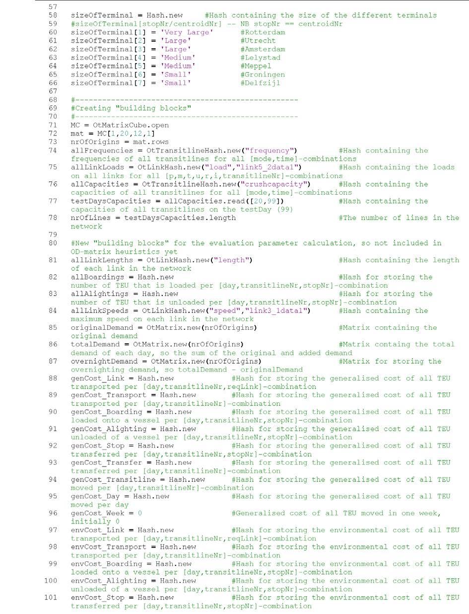
116 100

117 101

118 102

119 103

120 104

121 105

122 106

123 Appendix E. Detailed validation of four basic scenarios In Section 4.1 it was explained that a validation of the model is needed to assure it functions correctly and to check whether its results are viable and therefore useful. This validation process is performed by checking several basic scenarios in the model, for each of which the output can be checked with separate (manual) calculations. A more detailed discussion of each of these four scenarios, the separate calculations and how these compare to the output of the model, can be found in this Appendix. 1) An empty running IIWT service line This first scenario is checked on the Sunday of the modelled week: Sl1 runs once that day, but it does so empty, because there is no freight transport demand that day. Normally this situation would not arise, because the service schedule is deduced from the freight transport demand throughout the week. However in theory it is possible that a vessel needs to return empty due to an imbalance in the to/from-ratio. In addition the results of this scenario are useful for comparison with those of the next scenario, that includes fully loaded vessels. The output shows that the total transported time on Sunday is 0.0 hours for both scenarios, which corresponds with the fact that there is no transportation of containers. This lack of containers also means that there are no transfers and thus the costs solely depend on the transportation costs, which can be checked separately with the help of Equations 4.4 and 4.8. For the scenario with Rhine- Herne vessels this gives the following results: Total Gen_monetary_cost = 3.99 * 100 = 399 euro Total Gen_environmental_cost = 5.45 * 100 = 545 euro And for the scenario with Rhine vessel these values become: Total Gen_monetary_cost = 5.50 * 100 = 550 euro Total Gen_environmental_cost = 5.45 * 100 = 545 euro These values all correspond with the output of the model and therefore it is concluded that unloaded vessels are handled sufficiently accurate. 2) Direct transport with one constant load The Monday of the simulated week is used to check the second scenario. In this case both Sl1 and Sl2 run once, Sl1 should transport a load equal to its capacity and Sl2 should transport a load equal to half its capacity, and both should do so from their respective starting point to their destination. The costs again can be calculated using Equations 4.4 and 4.8. In a similar way the total transport time for each of the service lines can be calculated, based on the summation of the time needed for the transfers, for which Equation 4.3 is used, and the time needed for transport. For the scenario with Rhine-Herne vessels this means that the total cost and transport time of Sl1 becomes: Total Gen_monetary_cost = ( 77*90* 2 ) + + *100* = = euro 107

124 5.45 Total Gen_environmental_cost = ( 0.02*90*2 ) + *100*90 90 = = euro Total transport time = * + 1 * *90*2 * = = 1023 hours For the same scenario the costs and transport time of Sl2 are: Total Gen_monetary_cost = ( 77* 45* 2 ) + + *100* = = 7525 euro 5.45 Total Gen_environmental_cost = ( 0.02* 45* 2 ) + *100* = = euro Total transport time = * + 1 * * 45* 2 * = = 444 hours For the scenario with the Rhine vessels the total costs and transport time of Sl1 become: Total Gen_monetary_cost = ( 77* 208* 2 ) + + *100* = = euro 5.45 Total Gen_environmental_cost = ( 0.02* 208* 2 ) + *100* = 8, = euro 108

125 Total transport time = * + 1 * * 208* 2 * = = hours And finally the costs and transport time for Sl2 in this scenario can be calculated: Total Gen_monetary_cost = ( 77*104* 2 ) + + *100* = = euro 5.45 Total Gen_environmental_cost = ( 0.02*104*2 ) + *100* = = euro Total transport time = * + 1 * *104*2 * = = hours The output of the model presents the same results as these calculations and therefore the way the model handles (fully) loaded vessels is also considered sufficiently accurate. 3) Indirect transport with one constant load In this third scenario it is validated if indirect transportation, so routes that require a transfer, are handled correctly by the model. To keep the scenario transparent, it is assumed that there is no intermediate (un)loading, which means that the load is transported from its origin to its destination in its original composition, so no containers are added to or taken out of this load. This scenario is checked on Wednesday and Thursday of the modelled week: on Wednesday Sl1 runs once and should transport a load equal to its capacity from T1 to its transfer point T2 and on Thursday Sl2 runs once and should transport this same load from T2 to its final destination T3. The total costs can be calculated the same way as before, however for the calculation of transport time extra time needs to be added to account for the time spent at T2 by the containers after their arrival on Wednesday and before their departure on Thursday. As was explained in Section 4.1 this is done by adding a waiting time of 24 hours for each container. The combined costs and transport time for the entire trip from T1 to T3 via T2 for the scenario with Rhine-Herne vessels thus are equal to: 109

126 Total Gen_monetary_cost = ( 77*90* 4 ) + + * 2*100* = = euro 5.45 Total Gen_environmental_cost = ( 0.02*90* 4 ) + * 2*100*90 90 = = euro *100 Total transport time = * + 1 * *90*4 *90 24* = = 4206 hours ( ) And when performing the same calculations for the scenario with Rhine vessels, the combined costs and transport time should be equal to: Total Gen_monetary_cost = ( 77* 208* 4 ) + + * 2*100* = = euro 5.45 Total Gen_environmental_cost = ( 0.02* 208* 4 ) + * 2*100* = = euro *100 Total transport time = * + 1 * * 208* 4 * * = = hours ( ) The results that can be found in the output of the model are in concurrence with these calculated values and therefore it is concluded that the model also is sufficiently capable of handling indirect transport. 4) Direct transport with a change in the load In this fourth and final scenario the model is validated for intermediate unloading. This case is set up by letting Sl3 run once on Friday: the vessel is loaded with a full load at T3, then ships to T2, where it unloads half its load, after which it continues towards T1, where the other remaining half of the containers are unloaded. The costs are still calculated with the same formulas, but the calculation of the transport time is 110

127 slightly different. Though there is no waiting time due to indirect transport, the waiting time of the containers that are already aboard the vessel during the unloading at T2 should be factored in. The resulting calculations for the scenario with a Rhine-Herne vessel thus become: Total Gen_monetary_cost = ( 77* 45* 2) + ( 77*90 ) + + *100* *100* = = euro 5.45 Total Gen_environmental_cost = ( 0.02* 45* 2) + ( 0.02*90 ) + *100* *100*90 90 = = euro Total transport time = * + 1 * *90 * 1 * *45* *90 + * * * = = 1398 hours And when performing these same calculations for the scenario with a Rhine vessel, the results are: Total Gen_monetary_cost = ( 77*104* 2) + ( 77* 208 ) + + *100* *100* = = euro 5.45 Total Gen_environmental_cost = ( 0.02*104* 2) + ( 0.02* 208 ) + *100* *100* = = euro 111

128 Total transport time = * + 1 * *208 + * + 1 * *104* * * * * = = hours When comparing the results of these calculations with the output of the model, it becomes clear that this fourth and final scenario, which checks the model s capability for handling direct transport with a change in the load, is also handled sufficiently accurate. 112

129 Appendix F. The output of the validation simulations As explained in Section 4.1 and Appendix E a network was created for the sole purpose of validating the model. The output of the model for this network in combination with Rhine-Herne vessels and with Rhine vessels is presented in Boxes 6 and 7 respectively. Box 6: Output of the simulation of the validation network in combination with Rhine-Herne vessels. 113

130 114

131 115

132 116

133 117

134 118

135 Box 7: Output of the simulation of the validation network in combination with Rhine vessels. 119

136 120

137 121

138 122

139 123

140 124

141 Appendix G. Basic network: OD-Matrices Table 25: OD-matrix for Sundays in the small terminals scenario of the basic network. Source of data: own data. Table 26: OD-matrix for Mondays, Wednesdays, and Fridays in the small terminals scenario of the basic network. Source of data: own data. Table 27: OD-matrix for Tuesdays and Thursdays in the small terminals scenario of the basic network. Source of data: own data. Table 28: OD-matrix for Saturdays in the small terminals scenario of the basic network. Source of data: own data. 125

142 Table 29: OD-matrix for Sundays in the medium terminals scenario of the basic network. Source of data: own data. Table 30: OD-matrix for Mondays, Wednesdays, and Fridays in the medium terminals scenario of the basic network. Source of data: own data. Table 31: OD-matrix for Tuesdays and Thursdays in the medium terminals scenario of the basic network. Source of data: own data. Table 32: OD-matrix for Saturdays in the medium terminals scenario of the basic network. Source of data: own data. 126

143 Table 33: OD-matrix for Sundays in the large terminals scenario of the basic network. Source of data: own data. Table 34: OD-matrix for Mondays, Wednesdays, and Fridays in the large terminals scenario of the basic network. Source of data: own data. Table 35: OD-matrix for Tuesdays and Thursdays in the large terminals scenario of the basic network. Source of data: own data. Table 36: OD-matrix for Saturdays in the large terminals scenario of the basic network. Source of data: own data. 127

144 Table 37: OD-matrix for Sundays in the very large terminals scenario of the basic network. Source of data: own data. Table 38: OD-matrix for Mondays, Wednesdays, and Fridays in the very large terminals scenario of the basic network. Source of data: own data. Table 39: OD-matrix for Tuesdays and Thursdays in the very large terminals scenario of the basic network. Source of data: own data. Table 40: OD-matrix for Saturdays in the very large terminals scenario of the basic network. Source of data: own data. 128

145 Appendix H. Basic network: Design of the service line schedules As explained in Section 4.2 the service line schedule for each of the network scenarios is derived from the freight transport demand, rather than making it constant or a variable with a range of values. As a consequence a service schedule needs to be designed for each network type terminal size combination; this scheduling process is discussed in the first paragraph of this Appendix. The next three paragraphs each discuss the service schedules of one of the three network types for the basic network, the results for these schedules on the basic network with the distance between the port and the hinterland, and the distance between the inland terminals both set to 50 km, and the final choice for a service schedule per network type terminal size scenario combination. Creating a service line schedule The freight transport demand forms the starting point for the service line schedule: for each of the service lines that run in a certain network type it can be calculated how many TEUs need to be transported over the week as a whole, as well as on the different days of the week. On a single day the capacity does not necessarily has to be equal to or larger than the demand, however is should be on a weekly basis to prevent a build-up of containers in the network. The daily differences are not calculated separately, but instead are linked: if there is a shortage on day X, the remaining demand is added to that of the next day. So daily shortages are accumulated, whereas daily surpluses are not. Instead these are used to diminish any remaining shortages, after which a weekly pattern will arise. As an example, these calculations of the first alternative of the BE Network - small terminals combination are presented in Table Table 41: Example of the calculation of the compounded differences between the daily capacity and demand for the first alternative of the BE Network - small terminals combination. Day of the week Demand per service line [TEU] Frequency [-] Capacity [TEU] Compounded difference capacity demand [TEU] Sunday Monday 32 1x Tuesday Wednesday 32 1x Thursday Friday 32 1x Saturday Source of data: own data. The service schedule design is optimised by minimising the difference between the total weekly capacity and transport demand, as well as the differences between the daily capacity and transport demand for each of the service lines. However the service schedule that has the smallest weekly capacity surplus is not also necessarily the service schedule in which daily differences are the smallest, which is why two alternatives are created for each network type - terminal size combination. Then, using the evaluation parameters, time, environmental friendliness, and costs, the performance of both of these schedules is compared and a final choice for either one is made. 13 Due to the transport demand and the design of the BE network, all service lines in this scenario have to transport the same amount of containers on the different days of the week. As a consequence the calculations only have to be performed once and all service lines can be optimised at the same time. 129

146 Before the alternatives for the different network types are discussed, a final note should be made about the accuracy of this method. As noted in Section 3.3 and explained in Appendix C the model performs the OD-matrix heuristics for capacity problems suboptimal. Due to the origin of this error, this effect gets stronger as the number of stops in a service line increases. Because the L Network service line has three intermediate stops in its service line and those of the BE and HS Network do not have any intermediate stops at all, this effect is stronger in the L Network. As a result a larger margin is needed in the L Network service schedules, not because the actual demand requires this, but because the error caused by the model does. Therefore the service schedules of the L Network are suboptimal and as a consequence so are the networks performances a fact that needs to be taken into account in the final evaluation of the different network types. BE Network The two considered service schedules for the BE Network for each of the terminal size scenarios are presented in Table 42, whereas their performance for each of the three evaluation parameters can be found in Table 43. Based on these results a decision for one of the two alternatives can be made per terminal size scenario: Small terminals When comparing the results it becomes clear that the first alternative has a higher total generalised and environmental cost, 103% and 297% of the results of the second alternative respectively, but a lower total transport time, 24% of the total transport time of the other service schedule. Though these results do not present a clear outcome, they do show that the total transport time of alternative 2 is more than 4 times as high of that of alternative 1, whereas the environmental cost is only 3 times as low. Combined with the fact that the goal of the IIWT networks is to offer a regular high-quality alternative to potential clients, it therefore is decided to continue with alternative 1. Medium terminals The results of the medium terminals scenario show that the total generalised and environmental cost of alternative 1 are higher than those of alternative 2 (103% and 199% respectively), whereas the total transport time is lower (37%). Following the same reasoning as for the small terminals scenario, it is concluded that alternative 1 is the preferred service schedule. Large terminals The results for the large terminals scenario clearly show that the first alternative is preferable; both alternatives have the same total environmental cost, whereas the total generalised cost and total transport time are lower for alternative 1. Very large terminals Similar to the large terminals scenario, the results of the very large terminals scenario show that alternative 1 performs better than the second alternative; again the total generalised cost and total transport time of the first alternative are lower than those of the second alternative, whereas the environmental cost of both is the same. 130

147 Table 42: Overview of the service schedules that were created for the BE Network; per terminal-size-scenario two alternatives were considered. Service schedule alternatives BE Network [Frequency x Capacity in TEU] S Terminals M Terminals L terminals XL Terminals Alt. 1 Alt. 2 Alt. 1 Alt. 2 Alt. 1 Alt. 2 Alt. 1 Alt. 2 Sunday Monday 1 x 90 1 x x 90 1 x 90 2 x 90 1 x x 90 4 x 90 Tuesday x 90-3 x 90 1 x x 90 2 x 208 Wednesday 1 x 90-1 x 90 1 x x 90 1 x x 90 1 x 208 Thursday x 90-3 x 90 2 x x 90 2 x 208 Friday 1 x 90-1 x 90 1 x x 90 1 x x 90 2 x 208 Saturday x 90-2 x 90 1 x 90 3 x 90 1 x 208 Source of data: own data. Table 43: Overview of the results for the evaluation parameters of the two considered service schedules for the BE Network scenarios with a distance of 50 km from the port to its hinterland and 50 km between two inland terminals. BE Network: distance port to hinterland 50 km distance between inland terminals 50 km S Terminals M Terminals L terminals XL Terminals Alt. 1 Alt. 2 Alt. 1 Alt. 2 Alt. 1 Alt. 2 Alt. 1 Alt. 2 Generalised Cost [ ] Environmental Cost [ ] Transport time [hours] Source of data: own data. HS Network Due to the design of the HS Network, the service lines in this type of network can be divided into two categories based on the number of containers they transport: the two lines that run between the port and the hub and the four lines that run between the hub and the spokes. For each of these groups of lines a service schedule needs to be made, which should be optimised not only separately, but as a whole as well. The considered schedules for the small and medium terminals scenarios can be found in Table 44, whereas the schedules for the large and very large terminals scenarios can be found in Table 45. The results of the schedules of all four scenarios can be found in Table 46 and these are discussed below: Small terminals Both alternatives produce the same total environmental cost, but alternative 1 has a lower total transport time and total generalised cost and therefore is the preferred service schedule for this scenario. Medium terminals Following the same reasoning as for the small terminals scenario it is decided that the first alternative is the better service schedule. 131

148 Large terminals For this third terminal size scenario the generalised cost of alternative 2 is lower than that of alternative 1, the total environmental cost for both alternatives is the same, and the total transport time of alternative 1 is lower than that of alternative 2. The decision for either one of the service schedule therefore is made based on the relative difference: the total generalised cost of alternative 1 is 100.2% of that of alternative 2, whereas the total transport time of alternative 1 is 98.5% of that of alternative 2. Therefore it is decided to continue with the first alternative service schedule for this scenario. Very large terminals The choice in this scenario is once again clear, because just like for the small and medium terminals scenarios, alternative 1 has a lower total generalised cost and total transport time than alternative 2, and both generate the same amount of environmental costs. Table 44: Overview of the service schedules that were created for the HS Network scenarios with S and M terminals; per terminal-size-scenario two alternatives were considered. Service schedule alternatives HS Network [Frequency x Capacity in TEU] S Terminals M terminals Alt. 1 Alt. 2 Alt. 1 Alt. 2 Port - Hub Hub - Spokes Port - Hub Hub - Spokes Port - Hub Hub - Spokes Port - Hub Hub - Spokes Sunday Monday 1 x 90 1 x 90 1 x 90 3 x 90 1 x 90 1 x x 90 Tuesday 1 x 90 1 x 90 1 x 90 3 x 90 1 x 90 2 x x 90 Wednesday 1 x 90 1 x 90 1 x 90 3 x 90 1 x 90 1 x x 90 Thursday 2 x 90 2 x 90 1 x 90 3 x 90 1 x 90 2 x x 90 Friday 1 x 90 1 x 90 1 x 90 3 x 90 1 x 90 1 x x 90 Saturday 1 x 90 1 x 90 1 x 90 2 x 90 1 x 90 1 x 90 1 x 90 Source of data: own data. Table 45: Overview of the service schedules that were created for the HS Network scenarios with L and XL terminals; per terminal-size-scenario two alternatives were considered. Service schedule alternatives HS Network [Frequency x Capacity in TEU] L Terminals XL terminals Alt. 1 Alt. 2 Alt. 1 Alt. 2 Port - Hub Hub - Spokes Port - Hub Hub - Spokes Port - Hub Hub - Spokes Port - Hub Hub - Spokes Sunday Monday 3 x x 90 7 x 90 2 x x 90 2 x 90 4 x x 90 Tuesday 3 x x 90 9 x 90 2 x x 90 4 x 90 6 x x 90 Wednesday 3 x x 90 6 x 90 3 x x 90 5 x 90 5 x x 90 Thursday 4 x x 90 9 x 90 2 x x 90 4 x 90 6 x x 90 Friday 3 x x 90 7 x 90 3 x x 90 5 x 90 5 x x 90 Saturday 5 x 90 2 x 90 4 x 90 2 x 90 7 x 90 3 x 90 3 x x 90 Source of data: own data. 132

149 Table 46: Overview of the results for the evaluation parameters of the two considered service schedules for the HS Network scenarios with a distance of 50 km from the port to its hinterland and 50 km between two inland terminals. HS Network: distance port to hinterland 50 km distance between inland terminals 50 km S Terminals M Terminals L terminals XL Terminals Alt. 1 Alt. 2 Alt. 1 Alt. 2 Alt. 1 Alt. 2 Alt. 1 Alt. 2 Generalised Cost [ ] Environmental Cost [ ] Transport time [hours] Source of data: own data. L Network In the L Network all demand is transported via a single service line, the alternative service schedules of which can be found in Table 47. The performance of the service schedules for the different freight terminal size scenarios is presented in Table 48 and discussed in the remainder of this paragraph. Small terminals The first alternative has a higher total generalised and environmental cost than the second one (100.9% and 119.9% respectively), but a lower total transport time (76.1%). As explained the goal of the networks is a high quality and regular service and because the relative difference of the transport time between the two alternatives is bigger than that of the two types of costs combined, the decision is made in favour of the first service schedule. Medium terminals The first alternative has a lower total generalised cost and transport time than the second alternative (99.8% and 92.5% respectively) and the total environmental cost is the same for both alternatives. Therefore the first alternative is the preferred option of the two. Large terminals Again the first alternative has a lower total generalised cost and transport time (99.8% and 98.8% respectively) and the same total environmental cost as the second alternative, making it the better alternative of the two. Very large terminals The total environmental cost is the same for both alternatives, but the total generalised cost of the second alternative is lower than that of the first alternative (99.6%) and the total transport time of the first is lower than that of the second (98.1%). Following the same logic as before, the advantage of the lower total transport time outweighs the higher total generalised cost and thus the first alternative is chosen. 133

150 Table 47: Overview of the service schedules that were created for the L Network; per terminal-size-scenario two alternatives were considered. Service schedule alternatives L Network [Frequency x Capacity in TEU] S Terminals M Terminals L terminals XL Terminals Alt. 1 Alt. 2 Alt. 1 Alt. 2 Alt. 1 Alt. 2 Alt. 1 Alt. 2 Sunday Monday 1 x 90 3 x 90 1 x x 90 3 x x x 208 Tuesday 1 x 90 1 x x 90 2 x x x 90 6 x x 90 Wednesday 1 x 90 1 x 90 3 x 90 1 x x x x x 90 Thursday 1 x x 90 4 x 90 4 x 90 4 x x x x 90 Friday 1 x 90 1 x 90 3 x 90 1 x x 90 3 x x x 90 Saturday 1 x 90 1 x x 90 2 x 90 2 x x x x 208 Source of data: own data. Table 48: Overview of the results for the evaluation parameters of the two considered service schedules for the L Network scenarios with a distance of 50 km from the port to its hinterland and 50 km between two inland terminals. L Network: distance port to hinterland 50 km distance between inland terminals 50 km S Terminals M Terminals L terminals XL Terminals Alt. 1 Alt. 2 Alt. 1 Alt. 2 Alt. 1 Alt. 2 Alt. 1 Alt. 2 Generalised Cost [ ] Environmental Cost [ ] Transport time [hours] Source of data: own data. 134

151 Appendix I. Basic network: Detailed results This appendix contains more detailed versions of the results of the scenarios for the basic network that are discussed in Section 4.3. The results are presented in twofold: graphically in a total of nine graphs, each of which presents the performance of one of the network types for one of the three evaluation parameters for all scenarios, and numerically in four tables, each of which contains the numerical values of the results for one of the terminal size scenarios. The graphs are presented in three clusters, one for each of the network types, and the tables can be found at the end of this appendix. Begin-and-end network The results of the BE Network for are presented graphically in Figures 23, 24 and 25 below. These figures present the average transport time per TEU, the average environmental cost per TEU, and the average generalised cost per TEU respectively for all considered scenarios. Figure 23: The average transport time of the BE Network for all scenarios. (Own figure data from Tables 49-52) 135

152 Figure 24: The average environmental cost of the BE Network for all scenarios. (Own figure data from Tables 49-52) Figure 25: The average generalised cost of the BE Network for all scenarios. (Own figure data from Tables 49-52) 136

153 Hub-and-spoke network Just like for the BE Network the results for the average transport time per TEU, the average environmental cost per TEU, and the average generalised cost per TEU for all considered scenarios for the HS Network are presented graphically in Figures 26, 27 and 28 respectively. Figure 26: The average transport time of the HS Network for all scenarios. (Own figure data from Tables 49-52) Figure 27: The average environmental cost of the HS Network for all scenarios. (Own figure data from Tables 49-52) 137

154 Figure 28: The average generalised cost of the HS Network for all scenarios. (Own figure data from Tables 49-52) Line network The graphical representation of the results of the three evaluation criteria for all considered scenarios for the L Network can be found in Figures 29, 30 and 31 below. Figure 29: The average transport time of the L Network for all scenarios. (Own figure data from Tables 49-52) 138

155 Figure 30: The average environmental cost of the L Network for all scenarios. (Own figure data from Tables 49-52) Figure 31: The average generalised cost of the L Network for all scenarios. (Own figure data from Tables 49-52) The numerical values of the results The results numerical values are presented in four tables, which can be found on the following pages: Table 49 presents the results for the small terminals scenario, Table 50 for the medium terminals scenario, Table 51 for the large terminals scenario, and Table 52 for the very large terminals scenario. 139

156 Table 49: Overview of the results for the BE, HS, and L Network in the small terminals scenario. Source of data: own data. 140

157 Table 50: Overview of the results for the BE, HS, and L Network in the medium terminals scenario. Source of data: own data. 141

158 Table 51: Overview of the results for the BE, HS, and L Network in the large terminals scenario. Source of data: own data. 142

159 Table 52: Overview of the results for the BE, HS, and L Network in the very large terminals scenario. Source of data: own data. 143

160 Appendix J. Port of Amsterdam case study: OD-Matrices This appendix contains the yearly freight transport demand for the three growth scenarios of the case study (i.e. Tables 53, 54, and 55), as well as the OD-matrices for the three network types that are derived from these yearly demands. As explained in Section 4.4 it is important to note that not all yearly freight transport demand is included in the OD-matrices, because these freight flows are incidental and therefore not within the scope of the study. The OD-pairs for which the yearly freight transport demand is ignored are: From centroid 3 to centroid 2, From centroid 3 to centroid 4, From centroid 3 to centroid 7, From centroid 6 to centroid 3, From centroid 7 to centroid 3, And from centroid 7 to centroid 5. Table 53: Yearly freight transport demand for the low growth scenario of the case study. Source of data: CBS (2013). Table 54: Yearly freight transport demand for the normal growth scenario of the case study. Source of data: CBS (2013). Table 55: Yearly freight transport demand for the high growth scenario of the case study. Source of data: CBS (2013). 144

161 Table 56: OD-matrix for Sundays in the low growth scenario of the case study. Source of data: CBS (2013). Table 57: OD-matrix for Mondays, Wednesdays, and Fridays in the low growth scenario of the case study. Source of data: CBS (2013). Table 58: OD-matrix for Tuesdays and Thursdays in the low growth scenario of the case study. Source of data: CBS (2013). Table 59: OD-matrix for Saturdays in the low growth scenario of the case study. Source of data: CBS (2013). 145

162 Table 60: OD-matrix for Sundays in the normal growth scenario of the case study. Source of data: CBS (2013). Table 61: OD-matrix for Mondays, Wednesdays, and Fridays in the normal growth scenario of the case study. Source of data: CBS (2013). Table 62: OD-matrix for Tuesdays and Thursdays in the normal growth scenario of the case study. Source of data: CBS (2013). Table 63: OD-matrix for Saturdays in the normal growth scenario of the case study. Source of data: CBS (2013). 146

163 Table 64: OD-matrix for Sundays in the high growth scenario of the case study. Source of data: CBS (2013). Table 65: OD-matrix for Mondays, Wednesdays, and Fridays in the high growth scenario of the case study. Source of data: CBS (2013). Table 66: OD-matrix for Tuesdays and Thursdays in the high growth scenario of the case study. Source of data: CBS (2013). Table 67: OD-matrix for Saturdays in the high growth scenario of the case study. Source of data: CBS (2013). 147

164 Appendix K. Port of Amsterdam case study: Service schedules The service schedules of the Port of Amsterdam case study are derived in the same way as those of the basic network this process is described in Appendix H. The only difference is that for the case study the to/from ratio is not necessarily 50/50. Therefore for each pair of service lines the direction with the highest total freight transport demand is considered normative and used as input for the schedule. Begin-and-end network The BE Network consists solely of service lines connecting two terminals. The service schedule of the BE Network therefore consists of 7 x 2 service lines. The tables below present these schedules, as well as which centroids are connected by which pair of service lines. Table 68: Overview of the service schedule for the BE Network in the low growth scenario of the case study. Service schedule case study BE Network Low growth [Frequency x Capacity in TEU] Service lines 1&2 3&4 5&6 7&8 9&10 11&12 13&14 Centroids Sunday Monday 2 x 90 2 x x 90 3 x 90 1 x Tuesday 1 x x 90 2 x 90 5 x 90 1 x 90 1 x 90 1 x 90 Wednesday 2 x 90 4 x 90 1 x 90 4 x 90 1 x 90 1 x 90 - Thursday 3 x 90 6 x 90 2 x 90 5 x 90 2 x 90 1 x 90 1 x 90 Friday 2 x 90 4 x 90 1 x 90 4 x 90 1 x Saturday 1 x 90 3 x 90 1 x 90 3 x 90 1 x 90 1 x 90 1 x 90 Source of data: own data. Table 69: Overview of the service schedule for the BE Network in the normal growth scenario of the case study. Service schedule case study BE Network Normal growth [Frequency x Capacity in TEU] Service lines 1&2 3&4 5&6 7&8 9&10 11&12 13&14 Centroids Sunday Monday 1 x x 90 1 x 90 4 x 90 1 x Tuesday 3 x 90 7 x 90 2 x 90 6 x 90 2 x 90 1 x 90 1 x 90 Wednesday 1 x x 90 1 x 90 2 x x 90 1 x 90 - Thursday 3 x 90 7 x 90 2 x 90 6 x 90 2 x 90 1 x 90 1 x 90 Friday 1 x x 90 2 x 90 2 x x 90 1 x 90 1 x 90 Saturday 2 x 90 3 x 90 1 x 90 3 x 90 1 x 90 1 x 90 1 x 90 Source of data: own data. 148

165 Table 70: Overview of the service schedule for the BE Network in the high growth scenario of the case study. Service schedule case study BE Network High growth [Frequency x Capacity in TEU] Service lines 1&2 3&4 5&6 7&8 9&10 11&12 13&14 Centroids Sunday Monday 2 x 90 6 x 90 2 x 90 5 x 90 1 x 90 1 x 90 - Tuesday 4 x 90 7 x 90 2 x 90 7 x 90 2 x 90 1 x 90 1 x 90 Wednesday 2 x 90 6 x 90 2 x 90 5 x 90 1 x 90 1 x 90 - Thursday 4 x 90 8 x 90 2 x 90 7 x 90 1 x x 90 1 x 90 Friday 1 x x 90 2 x 90 5 x 90 2 x 90 1 x 90 1 x 90 Saturday 2 x 90 4 x 90 1 x 90 3 x 90 1 x 90 1 x 90 1 x 90 Source of data: own data. Hub-and-spoke network The HS Network consist of 3 service line pairs: one connecting the port (i.e. Rotterdam) to the hub (i.e. Amsterdam) via Utrecht, one from the hub to the northern most terminals (i.e. Groningen and Delfzijl), and one from the hub to Meppel via Lelystad. Again the different tables present the service line schedules, along with an overview of which pair of service lines connects which terminals. Table 71: Overview of the service schedule for the HS Network in the low growth scenario of the case study. Service schedule case study HS Network Low growth [Frequency x Capacity in TEU] Service lines 1&2 3&4 5&6 Centroids Sunday Monday 10 x 90 4 x 90 2 x 90 Tuesday 13 x 90 6 x 90 2 x 90 Wednesday 10 x 90 4 x 90 2 x 90 Thursday 6 x x 90 2 x 90 Friday 10 x 90 4 x 90 2 x 90 Saturday 3 x x 90 1 x 90 Source of data: own data. Table 72: Overview of the service schedule for the HS Network in the normal growth scenario of the case study. Service schedule case study HS Network Normal growth [Frequency x Capacity in TEU] Service lines 1&2 3&4 5&6 Centroids Sunday Monday 12 x 90 5 x 90 1 x 208 Tuesday 15 x 90 6 x 90 1 x 208 Wednesday 12 x 90 5 x 90 1 x 208 Thursday 16 x 90 7 x 90 1 x 208 Friday 12 x 90 5 x 90 1 x 208 Saturday 7 x 90 3 x 90 2 x 90 Source of data: own data. 149

166 Table 73: Overview of the service schedule for the HS Network in the high growth scenario of the case study. Service schedule case study HS Network High growth [Frequency x Capacity in TEU] Service lines 1&2 3&4 5&6 Centroids Sunday Monday 14 x 90 6 x 90 2 x 90 Tuesday 17 x 90 7 x 90 3 x 90 Wednesday 14 x 90 6 x 90 1 x 208 Thursday 17 x 90 7 x 90 3 x 90 Friday 14 x 90 6 x 90 2 x 90 Saturday 9 x 90 4 x 90 2 x 90 Source of data: own data. Line network The L Network consists of only two service lines, one from the port (i.e. Rotterdam) to the northern most terminal (i.e. Delfzijl) via all other terminals, and one in the opposite direction. The table below presents the service schedule for all three freight transport demand growth scenarios. Table 74: Overview of the service schedule for the L Network of the case study. Service schedule case study L Network [Frequency x Capacity in TEU] Growth scenario Low Normal High Service lines 1&2 1&2 1&2 Centroids Sunday Monday 10 x x x 90 Tuesday 14 x x x 90 Wednesday 10 x x x 90 Thursday 14 x x x 90 Friday 10 x x x 90 Saturday 7 x 90 8 x 90 9 x 90 Source of data: own data. 150

167 Appendix L. Port of Amsterdam case study: Numerical results Table 75: Overview of the numerical results of the model for the Port of Amsterdam case study. Source of data: own data. 151

168 Appendix M. Sensitivity analysis of the results Though in theory a sensitivity analysis should be conducted in a thorough manner, using for example linear regression models (Kleijnen, 2004) this would become a too extensive task for this research. Therefore a more hands-on, first impression kind of approach is used: instead of performing an extensive analysis of only one or two variables in the model, a short analysis is performed for as much of the seemingly influential variables in the network as possible. As a result the approach that is used varies at times, but the end results does provide a first estimate of which variables might require further investigation in future research. Changing the input variables of the model Section 4.1 introduced a number of variables that are used in the calculation of the results for the three evaluation criteria, time, environmental friendliness, and costs. For each of these variables a value was chosen based on data from practice and literature. However these values could be off or could change due to circumstances, such as an increase in fuel prices or emission pricing. Therefore it is valuable to investigate what sort of effect these kind of changes would have on the results. To do so two scenarios were made: one in which all the values of the variables are lowered by 25% and one in which they are increased by 25%. Table 76 presents an overview of the variables and their respective values. The two scenarios have been run for the transport distance scenario with a main haul distance of 100 kilometre and a distance of 50 kilometre between inland terminals, in combination with all four terminal size scenarios and all three network types. The results for these two scenarios can be found in Table 77 on the next page alongside the results for the original values. Table 76: Overview of the values used in the sensitivity analysis of the variables of the evaluation criteria calculation. Source of data: Bak et al. (as cited in Beelen, 2011); Van Duin and Geerlings, 2008; Environmental and Energy Study Institute, 2012; Fusion Media Limited, 2013; Harms and Willigers, 2002; Hüsig et al. 2005; Liebherr, 2013; Wiegmans and Konings, These results show that the average generalised cost per TEU responds directly to the changes: for all terminal size scenarios and network types it increases/decreases by exactly 25%. Given the fact that all variables that contribute to the average generalised cost per TEU have also been changed by 25%, this seems logical. 152

169 Table 77: The results for the BE, HS, and L Network for low, regular, and high values of the input variables. Source of data: own data. 153

170 The average environmental cost per TEU increases with about 25 to 26% and decreases with about 24 to 25%. This might seem strange, because just like the average generalised cost per TEU, all variables that contribute to it have been changed by 25%. However the values for the environmental cost of a transfer are so small, that due to rounding off the increase and decrease are not always 25%, but sometimes larger or smaller. And because the contribution of transfers to the average environmental cost per TEU is relatively small, the effect of this error is only about 1%. Unlike the other two criteria, something different happens with the average transport time per TEU: the results do increase and decrease along with the input values, but the response is variable and less than 25%. The increase and decrease is smaller for the smaller terminal size scenarios, but increases along with the terminal size. There also is a difference in the way the three network types respond: the BE Network shows the smallest response, 2 to 8%, the HS Network has only a slightly bigger response, 2.6 to 9.5%, and the L Network has the biggest response, 5.5 to 15.9%. These variances are caused by the overnighting containers that also contribute to the average transport time per TEU, but whose input does not change along with the other variables. The more containers are transported by a single service line, the relatively smaller the difference between the capacity of this service line and its demand becomes. In turn this means that relatively less containers have to wait due to a lack of capacity or because their service line does not run at all. Therefore the larger terminal size scenarios have a bigger response to the changes in the input than the smaller ones. It also explains why the L Network shows the biggest change in the results: it has only one service line, which transport all freight transport demand. The BE and HS Network on the other hand consist of more, but smaller service lines which cause relatively more overnighting containers. So the average generalised and environmental cost per TEU respond directly to a change in their input values, meaning that any improvements that can be made to the transfer or transport process would directly result in the same amount of savings. In addition the error of about 1% in the average environmental cost per TEU underlines that the contribution of transfers to this criterion is relatively small. And given the relatively small influence of the transport distance on the results of the average generalised cost per TEU, the opposite is most likely true for this criterion. However any changes in the input of the average transport time per TEU are damped by the overnighting containers. In case of unexpected delays this means that the actual effect on the average transport time is smaller than expected, but unfortunately it also means that any improvements made in the IIWT process result in a relatively small decrease of the average transport time per TEU. A smaller overnight time for the HS Network The average overnight time was set to 24 hours to resemble the day that containers have to wait at the terminal if there is no route or capacity available. However in the case of the HS Network the containers also have to wait at the hub and for this 24 hours is probably inaccurate. Especially for the large or very large terminals scenario this value in reality might be lower, because of the high frequency service schedule that is used in these scenarios: the containers at the hub do not have to wait an entire day for a connection. 154

171 Table 78: The results for the three network types, as well as those of the HS Network with an overnight time of 12 hours. Source of data: own data. Therefore the influence of a lower average overnight time on the performance of the HS network in the large and very large terminals scenarios has been investigated. For this purpose the average overnight time was set to 12 hours and the average transport time was calculated once more. The results can be found in Table 78 above, which presents both the standard results of the BE, HS, and L Network in the large terminals and very large terminals scenarios, as well as the results of the adapted HS Network in these scenarios. The results of the latter are labelled HS*. For the large terminals scenario the new average transport time ranges from to hours/teu, which means an improvement of 20 to 28%. The average transport time of the very large terminals scenario ranges from to hours/teu, which means a drop in the average transport time per TEU of 18 to 23%. So there is a substantial decrease in the average transport time per TEU of the HS Network: the HS Network and L Network now alternately have the highest average transport time per TEU in the large and very large terminals scenario. However it should be noted that the average transport time per TEU of the BE Network is still the lowest. The influence of the vessel capacity The influence of using Rhine or Rhine-Herne vessels on the results remains unclear. So far the service schedules have been designed to fit the freight transport demand best as possible. To get a better understanding of whether or not the use of a certain vessel type justifies a less (or more) optimal service schedule, their influence requires further investigation. Ideally this could be done by designing two service schedules, one exclusively with Rhine vessels, and one exclusively with Rhine- Herne vessels. Otherwise these schedules are designed regularly, so with as little overcapacity as possible. However for now only a first estimate of the impact is made. Especially for the environmental cost the influence of using one vessel type over the other might prove interesting, because the environmental cost per kilometre is the same for both vessel types. As 155

172 an example compare a service line that requires a total capacity of 600 TEU. When only Rhine vessels are scheduled the average environmental cost of transport per TEU would be equal to: 3 vessels * cost/km * distance 600 TEU Whereas the average environmental cost of transport per TEU of the same service lines with Rhine- Herne vessels would become: 7 vessels * cost/km * distance 600 TEU So the use of Rhine-Herne vessels over Rhine vessels could result in an average environmental cost of transport per TEU that is about 2.3 times as high. Further research would be needed to investigate the tipping point between the seemingly advantageous use of the Rhine vessels and a less efficient service schedule. A final note should be made regarding one of the model s limitations: currently it is only possible to use one type of vessel per day of the week. As a result the current model often forces the user to choose between a more efficient service schedule the chosen example provides an ideal situation in which the use of either vessel type results in almost the same overcapacity and the benefits of a larger vessel. Ideally this problem would be solved first, which would make finding the tipping point of the current model unnecessary. Very large transport distance Due to the relatively high generalised cost of transfers, the influence of the transport distance on the average generalised cost per TEU is small. However as the transport distance increases, its contribution to the average generalised cost per TEU increases, whereas that of the transfers remains equal. Therefore it could be that if a very large transport distance is implemented in the network, the average generalised cost per TEU becomes more influenced by (changes in) the transport distance. To investigate the effect of a very large distance a scenario was created with a distance of 400 kilometres from the port to its hinterland and with a distance of 100 kilometres between the different inland terminals. The results were recalculated for all network types and terminal size scenarios and can be found in Table 79 on the next page, which presents the results for the BE, HS, and L Network in three transport distance scenarios: the main haul distances in these scenarios are 100, 200, and 400 kilometres, and all three scenarios have a distance of 100 kilometres between inland terminals. It should be noted that such a large transport distance is not in accordance with the modelled time period (with a speed of 12 km/h approximately 300 kilometres is the maximum sailing range on one day) and the results should therefore only be used as a first estimate of this phenomenon. 156

173 Table 79: The results for the BE, HS, and L Network for the km, km, and km scenarios. Source of data: own data. 157

174 The results show an increase that is still in line with the other transport distance scenarios: the difference between the scenario and the scenario is twice as large as the difference between the scenario and the scenario which is to be expected because the transport distance is also twice as large but more importantly the relative size of this difference compared to the average generalised cost per TEU increases by only 1 to 6%. As a result it becomes clear that even with a main haul distance this large, the relative cost of transfers still outweighs that of the actual transport, and that the relative contribution of the actual transport on the average generalised cost per TEU remains small. The effect on the average environmental cost per TEU and the average transport time per TEU is as expected: the increase in the average environmental cost per TEU is considerable, but decreases as the terminal size increases, and the average transport time per TEU also shows an increase in line with the other transport distance scenarios. So these two evaluation criteria also show that a very large main haul distance is not yet sufficient to shift the balance in the relative contributions of the transfers and actual transport to any of the criteria. Adding time for (un)mooring to the model In the current calculation of the average transport time per TEU, the time required for (un)docking vessels before and after the actual loading process is not included. Including it in the calculation could have a substantial impact on the results, making vessels with a larger capacity and service schedules with fewer vessels relatively more interesting alternatives. However if it is assumed that the quay at terminals is long enough for a vessel to (un)moor while another vessel is being (un)loaded, the total (un)mooring time no longer depends on the number of vessels, but on the number of grouped stops in the service schedule. If we take the basic network as an example, the BE Network has 10 grouped stops 14, the HS Network also has 10 grouped stops 15, and the L Network has only 5 grouped stops 16. Implementation of the (un)docking time in the calculation of the average transport time per TEU would therefore relatively improve the performance of the L Network for this criterion compared to those of the BE and HS Network. The difference in the number of grouped stops between the BE and HS Network, and the L Network will increase if the number of terminals in the network increases as well. So if the time taken for (un)docking and the number of inland terminals in the network increases, the average transport time per TEU of the L Network will increase relatively less than that of the BE Network. Ultimately this could lead to a turning point, after which the L Network offers a lower average transport time per TEU than the BE Network. However there might be other factors in play that are also affected by the 14 There is 1 grouped stop at the port when loading the lines towards the hinterland, 3 at the inland terminals, when these 3 lines are unloaded, 3 more at the inland terminals when the lines towards the port are loaded, and finally 3 more, when these returning lines are unloaded at the port. 15 There are 6 service lines, each of which has 1 grouped stop for loading and 1 grouped stop for unloading, with the exception of the loading process at the hub, where the loading process of three lines can be combined. 16 There is 1 grouped stop at each of the inland terminals, because there is only one service line, of which the loading and unloading process is combined, and there are 2 grouped stops at the port, 1 for loading and 1 for unloading. 158

175 increase in the number of inland terminals, which could counteract or strengthen this effect. Therefore further investigation, including modelling of the (un)mooring time, is needed before a definitive conclusion on this topic can be made. Adding Forty-foot Equivalent Units to the model There always have been alternative intermodal load units other than the TEU, but the latter did become the industry standard. However with increasing freight flows larger containers grew more popular. The biggest increase in popularity can be found for the FEU, as the time series of the container throughput in the port of Rotterdam shows (Port of Rotterdam Authority, 2014). In the current model all cargo was considered to be TEUs, however adding FEUs could have a substantial impact, which can be illustrated with a small example: if two TEU are needed to transport amount X of cargo, only one FEU is needed to transport that same amount of cargo 17. As a result only one transfer is needed to load the cargo if the FEU is used, whereas two transfers are needed if the pair of TEUs is used. To investigate the impact of the FEU on the results, all code in the job scripts that uses the amount of TEU that is either loaded or unloaded is multiplied by the following factor: %_of_feu (1 - ) 2 So if the total freight transport demand is 100 TEU, and 20% consists of FEUs, only 90 transfers 18 are needed to load all demand aboard a vessel. This method is not perfect, because it assumes the FEUs are evenly spread over all freight transport demand and no preferential treatment for loading FEUs or TEUS occurs. However this method does provide a first insight in the consequences of adding FEUs to the model. With the addition of this factor, the results have been recalculated for the transport distance scenario with a distance of 100 kilometre between the port and its hinterland, and a distance of 50 kilometre between the inland terminals. The percentage of FEUs in the freight transport demand is set to 50%, which is an estimate based on the time series of the port of Rotterdam (Port of Rotterdam Authority, 2014) The results for the combination of all three network types and all four terminal size scenarios can be found in Table 80, along with the results for the regular model without FEUs. By setting the amount of FEUs in the freight transport demand to 50%, only 75% of the regular amount of transfers is needed. So depending on the relative influence of transfers on each of the evaluation criteria, a decrease of at the most 25% in the results could be observed: for the average generalised cost per TEU the decrease is 20.0 to 24.6%, for the average environmental cost per TEU it is 0.1 to 3.9%, and for the average transport time per TEU it amounts to 3.5 to 21.7%. 17 It is assumed that the weight of the cargo does not exceed the limitations of the FEU. 18 Of the 100 TEU freight transport demand, 80% consists of TEUs and 20% consists of FEUs. So in total 80 TEUs and 10 FEUs are transported, which means a total of 90 transfers is needed to load all the containers. 159

176 Table 80: Results of the sensitivity analysis regarding the addition of FEUs to the model in the km scenario. Source of data: own data. These differences are in line with the findings for the changes in the input variables. The average generalised cost per TEU responds strongly to the change in the number of transfers, because the actual transport has a relatively small contribution to this criterion, whereas the average environmental cost per TEU has only a small response, due to the relatively small influence of transfers on this criterion. The results for the average transport time per TEU are again the most varied: as the terminal size increases, the influence of the FEUs on the results does so as well, and the L Network has the biggest response, whereas the BE Network again has the smallest. The reason for these results is the same as for the change in the input variables of the evaluation criteria calculation. The average transport time per TEU of larger terminal size scenarios is relatively less influenced by overnighting containers than that of the smaller terminal size scenarios. This effect is also observed for the L Network, in which a single service line transports more freight, which relatively decreases the influence of the overnighting containers. All-in-all it seems that the influence of adding FEUs to the model indeed is substantial. Adding it to a future version of the model therefore is recommended. Though ideally this would be done in a more thorough manner, making it possible to distinguish two (or more) types of freight, which can be treated with different priorities. However if such a solution is not available, the current solution of adding a factor to the calculations will still give a good first insight in the FEUs influence. 160