City-Delta Phase 2. Final Report

Transcription

1 City-Delta Phase 2 Final Report C. Cuvelier, P. Thunis, R. Stern, N. Moussiopoulos, P. Builtjes, L. Rouil, M. Bedogni, L. Tarrason, M. Amann, C. Heyes Submitted to the European Commission Contract #B4-3040/2003/361392/MAR/C1 IIASA Contract No February 2005 International Institute for Applied Systems Analysis Schlossplatz 1 A-2361 Laxenburg, Austria Tel: Fax: info@iiasa.ac.at Web:

2 City-Delta Phase 2 Final Report C. Cuvelier and P. Thunis European Commission, Joint Research Centre, Institute for Environment and Sustainability, Ispra, Italy R. Stern Free University of Berlin, Germany N. Moussiopoulos Aristotle University Thessaloniki, Greece P. Builtjes TNO/MEP, Apeldoorn, The Netherlands L. Rouil INERIS, Paris, France M. Bedogni AMMA, Milan, Italy L. Tarrason EMEP, Oslo, Norway M. Amann and C. Heyes IIASA, Laxenburg, Austria Submitted to the European Commission Contract #B4-3040/2003/361392/MAR/C1 IIASA Contract No February 2005 This paper reports on work of the International Institute for Applied Systems Analysis and has received only limited review. Views or opinions expressed in this report do not necessarily represent those of the Institute, its National Member Organizations, or other organizations sponsoring the work.

3 Contents 1 Introduction 1 2 Background The policy context The objectives of the City-Delta project Set up of the project and methodology 5 3 Emission inventories Introduction Regional scale emissions: EMEP TNO City-scale emissions: General characteristics Merging city- and regional-scale emissions: Methodology Comparison of EMEP and city-scale emissions Biogenic emissions 15 4 Model results Scenarios Requested output 16 5 Analysis of the model output Mean summer (April-September) ozone (cf. Figure 5.1) Ozone exceedance days (60 ppb, 8hr average) (cf. Figure 5.2) Taylor diagram for mean summer ozone (cf. Figure 5.3) Annual mean PM 10 (cf. Figure 5.4) Taylor diagram: Annual mean PM 10 (cf. Figure 5.5) Delta (CLE-2000) mean summer ozone (cf. Figure 5.6) Delta (MFR-CLE) mean summer ozone (cf. Figure 5.7) Delta (CLE-2000) annual mean PM 10 (cf. Figure 5.8) Delta (MFR-CLE) annual mean PM 10 (cf. Figure 5.9) City-overview: Mean summer daytime ozone (cf. Figure 5.10) 19 iii

4 5.11 City-overview: SOMO35 indicator (cf. Figure 5.11) City-overview: Annual mean PM 10 (cf. Figure 5.12) City-overview: Annual mean PM 2.5 (cf. Figure 5.13) 20 6 Functional relationships to estimate urban air quality Analysis of observational data Data Sources Results Analysis of model results Functional relationships for the RAINS model Input data to the RAINS calculations Preliminary results Comparison with monitoring data 68 7 Implementation in the RAINS model 72 8 Summary 77 iv

5 1 Introduction The RAINS model addresses European scale air pollution with a spatial resolution of 50*50 kilometres, essentially dictated by the spatial resolution of the atmospheric dispersion model (i.e., the EMEP Eulerian model) whose results are incorporated into RAINS. For European-scale analysis, such a resolution is considered adequate for capturing the features of long-range transported pollutants and, with additional information, for conducting impact assessment with reasonable accuracy. However, it is clear that ambient concentrations of some air pollutants show strong variability at a much finer scale (e.g., in urban areas, in street canyons, at hot-spots close to industrial point sources of emission, etc.), and that at least some of these differences result in small-scale variations of pollution impacts on humans and the environment. Thus, there is a need that CAFE addresses air quality problems that occur on a finer scale than the 50*50 km grid mesh that is considered adequate for regional scale pollution. The City-Delta model intercomparison, initiated by IIASA in cooperation with the Institute for Environment and Sustainability of the Joint Research Centre (Ispra), MET.NO and EUROTRAC-2, has conducted a systematic comparison of regional scale and local scale dispersion models. The aim of this exercise is to identify and quantify the factors that lead to systematic differences between air pollution in urban background air and rural background concentrations. City-Delta explores systematic differences (deltas) between rural and urban background AQ, how these deltas depend on urban emissions and other factors, how these deltas vary across cities, and how these deltas vary across models. Based on the findings of City-Delta, the European Commission Environment Directorate General has set up a service contract B4-3040/361392/MAR/C1 City-Delta 2 with the objective to integrate the finding of the City-Delta project into the framework of the RAINS Integrate Assessment Model. The City-Delta 2 project has developed functional relationships that allow the estimation of urban levels of pollution (PM 2.5 ) as a function of rural background concentrations and local factors. The analysis addresses the response of health-relevant metrics of pollution exposure (i.e., mostly long-term concentrations with or without thresholds) towards changes in local and regional precursor emissions, including the formation of secondary inorganic aerosols. This enables the generic analysis of urban air quality for a large number of European cities based on information available in the RAINS model framework. This final report describes the results obtained from the City-Delta2 project, in which six urban-scale dispersion models have been used to explore common emission control scenarios for four European 1

6 cities in a coordinated way. Functional relationships have been developed and implemented in the RAINS model, so that for the purposes of the CAFE project the implication of Community-wide emission control measures on urban air quality can be assessed. 2

7 2 Background C. Cuvelier, P. Thunis 2.1 The policy context The Clean Air For Europe (CAFE) programme of the European Commission is a programme of technical analysis and policy development which will lead to the adoption of a thematic strategy on air pollution under the Sixth Environmental Action Programme in The major elements are outlined in the Communication on CAFE (COM(2001) 245). The programme was launched in Its aim is to develop a long-term, strategic and integrated policy advice to protect against significant negative effects of air pollution on human health and the environment. The CAFE programme has the following specific objectives: To develop, collect and validate scientific information relating to the effects of outdoor air pollution, emission inventories, air-quality assessment, emission and air-quality projections, costeffectiveness studies and integrated assessment modelling, leading to the development and updating of air-quality and deposition objectives and indicators and identification of the measures required to reduce emissions; To support the implementation and review the effectiveness of existing legislation, in particular the air-quality daughter directives, the decision on exchange of information, and national emission ceilings as set out in recent legislation, to contribute to the review of international protocols, and to develop new proposals as and when necessary; To ensure that the sectoral measures that will be needed to achieve air-quality and deposition objectives cost-effectively are taken at the relevant level through the development of effective structural links with sectoral policies; To determine an overall, integrated strategy at regular intervals which defines appropriate airquality objectives for the future and cost-effective measures for meeting those objectives; To disseminate widely the technical and policy information arising from the implementation of the programme. Among the problems that CAFE has to solve, the CAFE communication highlights ozone and Particulate Matter (PM) as priority pollutants. Both pollutants have adverse effects on human health. Ground-level ozone is due to atmospheric emissions of nitrogen oxides and volatile organic compounds that are transformed in photochemical reactions to ozone. Ozone attacks vegetation and materials and has a strong effect on human health, where exposure to high levels is clearly linked with 3

8 increased mortality in the population. The World Health Organisation (WHO) health guideline value of 120 µg/m 3 (eight-hour average) is widely exceeded in Europe. Recent evidence has shown that there are also health effects, such as deaths brought forward in time, below the WHO guideline value. The effects where found also at low ozone levels but at the lower levels the uncertainties of the relationship where larger. Particulate matter is emitted from combustion processes and mechanical wear, but also formed through atmospheric chemical and physical processes whereby the gas components are transformed into PM mass. In the case of PM there appears to be no concentration below which there are no effects on human health. There are many uncertainties and complexities related to the formation and transport, and the mechanisms of damage of these two pollutants. In order to address these challenges effectively (and that also means cost-effectively) it is clearly desirable to tackle the problems in the context of an integrated programme. It is in this policy context that the Institute for Environment and Sustainability (IES) of the Joint Research Centre (JRC) in Ispra has initiated the City-Delta project. The project is co-organised by IIASA (International Institute for Applied Systems Analysis, Laxenburg, Austria), The Norwegian Meteorological Institute (EMEP/MSC-W, Oslo, Norway), TNO-MEP-EUROTRAC (Apeldoorn, The Netherlands), and CONCAWE (Brussels, Belgium). The JRC-IES acted as co-ordinator of the project. 2.2 The objectives of the City-Delta project The City-Delta project is an open model-intercomparison exercise to explore the changes in urban airquality predicted by different atmospheric chemistry-transport- dispersion models in response to changes in urban emissions. City-Delta aims at the study of ambient levels of ozone and Particulate Matter (PM 2.5 and PM 10 ). In line with the CAFE programme, it is health-driven and consequently addresses metrics of long-term exposure to ozone, and fine (PM2.5) and coarse particles (particles between PM10 and PM2.5). Assessments of health as well as of vegetation impacts require information about the long-term exposure to the various air pollutants. For ozone, studies revealed relations between the extent of vegetation damage and the AOT40, i.e. the hourly ozone concentrations in excess of 40 ppb cumulated over the vegetation period (three or six months). The new evidence of ozone health impact at levels below 120 µg/m 3 has been captured in the accumulated exposure to ozone above a certain evaluation threshold the SOMO35 indicator (defined as the sum of the maxima of the daily 8-hr running average ozone concentration in excess of 35 ppb). For PM the major long-term health effect, increased mortality, are captured through the annual averages PM

9 City-Delta has the following specific objectives: To assess the performance of the participating models and compare them against available observational data from different cities; To identify the range of model responses towards emission reductions; To provide information on the effectiveness of Europe-wide emission controls compared to local measures; To provide quantitative information in relation to legal obligations, e.g. whether a certain trend in emissions will achieve air- quality limit values; To provide guidance on how urban air-quality could be included in a European-wide evaluation of the cost-effectiveness of emission control strategies. 2.3 Set up of the project and methodology After some preparatory discussions in 2001, the kick-off meeting of the City-Delta project took place at the JRC-IES (Ispra, February 2002). This meeting was attended by 45 participants, including experts in the fields of monitoring, emissions, meteorology, and modelling. Most of the EU Member States were represented as well as some of the Candidate Countries. During this meeting all the technical details were discussed. A Steering Group was formed and the JRC-IES was asked to coordinate all the City-Delta activities, including the collection and management of all input and output data, setting up a City-Delta Web site, the distribution of data to the participating modelling groups, the organisation of further workshops and to guarantee the scientific quality of the activities. After the kick-off meeting an open announcement for participation was widely distributed, and approximately 20 modelling groups reacted positively and expressed their preparedness to participate with a total of 40 different model configurations. The second Workshop was organised at IIASA (Vienna, June 2002), mainly to review and discuss the modelling input data (monitoring, emissions, and meteorological data). Monitoring data and highresolution emission data were prepared by the local authorities and processed by JRC-IES. Emission inventories were complemented by EMEP data. The meteorological input data was provided by Meteo France. The first results of the validation against 1999 data were presented. The third Workshop took place at the Institute of Environmental Protection (Katowice, December 2002). This meeting was dedicated to the 1999 validation results, and the discussion of the first results of the delta calculations (impact of emission reductions). During the fourth Workshop, which was organised by CEAM (Valencia, April 2003), an in-depth analysis and discussion took place concerning the delta calculations. This first phase of the City-Delta project revealed major differences between the modelled and observed PM mass concentrations. All 5

10 chemistry models that simulate the fate of the various chemical components of PM result in a serious underestimation of observed PM mass concentrations. However, models agree to a large extent on the fate of anthropogenic primary particles and secondary inorganic aerosols. The decision was taken to pay more attention to the impact on PM (PM 2.5, PM 10, SULF, NITR, AMMO) of the various emission-reduction scenarios. It was also decided to bring the high-resolution city emission inventories in line with the EMEP emissions by performing a sector-wise scaling of all the emitted components onto the EMEP values. This was called City-Delta second phase in order to distinguish these new runs from the set of runs with the unmodified emission city inventories. Based on the results of City-Delta I and the ability of the models to reproduce ozone and PM levels, a contract was set up with the following modelling groups: a. REM model, contact person: Dr R. Stern (Free University of Berlin, Germany). Model 03 (fine scale), Model 36 (coarse scale). b. OFIS model, contact person: Prof N. Moussiopoulos (Aristotle University Thessaloniki, Greece). Model 15 (fine scale). c. LOTOS model, contact person: Prof P. Builtjes (TNO/MEP, Apeldoorn, The Netherlands). Model 24 (fine), Model 25 (coarse scale). d. CHIMERE model, contact person: Dr L. Rouil (INERIS, Paris, France). Model 32 (fine scale), Model 31 (coarse scale). e. CAMx model, contact person: Dr M. Bedogni (AMMA, Milan, Italy). Model 34 (fine scale), 41 (fine scale). f. EMEP model, contact person: Dr L. Tarrason (EMEP, Oslo, Norway). Model 21 (coarse scale). The models e) and f) participated in this exercise using their own resources. Fine-scale models have a resolution of 5 or 10 km, coarse-scale models are at 50 km resolution. The fifth workshop, organised by JRC-IES in collaboration with ARPA-Basilicata, took place in Matera (October 2003). The results for City-Delta phase 1 were reported, a number of inconsistencies in the emission inventories were discussed and solutions were proposed. The final City-Delta Workshop took place at JRC-IES (Ispra) in October The workshop summarized the findings from the two phases of the City-Delta model intercomparison and reviewed a first implementation of the functional relationships that allow urban air quality to be addressed in a Europe-wide integrated assessment model. In order to cope with the enormous amount of input and output data that was produced, the JRC-IES developed an interactive visualisation tool based on the language IDL to view the monitoring data, the emissions and the proposed emission reductions, to visualise the intercomparison of the validation results, and the intercomparison of the delta calculations. 6

11 3 Emission inventories C. Cuvelier, P. Thunis 3.1 Introduction In the frame of this project, emission data were collected from different sources including both high spatial resolution information from the cities and low spatial resolution information to cover the regional background. In this section, an overview of the characteristics of these different sources of emission data is provided. The methodology to merge the regional and local scale emission inventories in order to provide the participants with a uniform emission data set is also discussed. Finally, the scaling procedure used in City-Delta2 to avoid inconsistencies between the local and regional emissions is presented. 3.2 Regional scale emissions: EMEP TNO EMEP total annual emissions were provided in the EMEP grid coordinate system (resolution of 50 km), for NO x, SO 2, NMVOC, CO, NH 3 whereas PM 2.5 and PM 10 were obtained from TNO with a similar resolution. A temporal disaggregation of these annual totals into hourly values has been achieved for gas phase species through monthly, daily and hourly temporal profiles prepared by IER for GENEMIS. Both the temporal profiles for monthly and daily variations are activity-sector and country dependent whereas hourly profiles are only sector dependent. Only monthly variations have been considered for PM including a country dependency but variations remain similar for all SNAP activity-sectors. Since EMEP-TNO gridded emissions were provided only as area totals per sector, point sources were accounted for by distributing the emissions at different heights depending on their activity sectors. 3.3 City-scale emissions: General characteristics The city scale emission inventories which have been provided for City-Delta differ significantly in their spatial coverage and resolution, time disaggregation, VOC split, and reference year. Although these inventories have been modified by the scaling procedure described in Section 3.5, we hereafter describe the main characteristics of the original emission datasets. Spatial coverage and resolution: City-Delta domains over which output data have been requested from the participants cover an area of 300 x 300 km 2 centred on the city of interest. Among the available inventories, only Paris covered this City-Delta output domain entirely with a spatial resolution of 3 km. For Berlin and Prague, approximately two thirds of the domain is covered, with a 7

12 spatial resolution of approximately 2 km for Berlin and 5 km for Prague. In the case of Milan, the fine scale emissions include the whole Lombardy region with a 5 km spatial resolution which represents about one third of the output domain. Pollutants: Emissions for CO, NO x, NMVOC and SO 2 were provided by all four cities, as was the case for CH 4 except for Prague. Emissions for NH 3 were only available for the cities of Milan and Paris. Estimates of PM emissions differ significantly in their degree of complexity from one city to another. They range from the rather complex estimates, as for Milan where PM factors are based on three different sets of emission factor sources (TNO-CEPMEIP, IIASA, Lombardy region) and include both point and area sources, to cities like Berlin where simple scaling factors are used between PM 10 and PM 2.5 or TSP depending on the activity sector. VOC Speciation: For all cities except Paris, NMVOCs have been split according to the speciation released by AEAT (AEAT/ENV/R/0545 report: Speciation of UK emissions of NMVOC, N.R. Passant, February 2002). This speciation provides a breakdown into 227 species for 9 SNAP sectors. The Paris NMVOC emissions have been split according to available literature information and partly from expert interviews. Reference year: All emission estimates received in the frame of the City-Delta project were based on years included in the period. In the case of Berlin, the reference year is region- and sectorspecific. Details for the other cities are available in Table 3.1 below. In Figure 3.1 the spatial distribution of the NO x traffic emissions for the different cities provides an illustration of the differences in resolution and spatial coverage of the emission inventories. Areas within the modelling domains (300x300 km 2 ) where fine scale emissions are not available have been filled with EMEP regional scale emissions so that the City-Delta modelling community received a complete and consistent set of emissions over each of the modelling domains. The detailed NO x emission sector-split for the different cities is illustrated in Figure 3.2. As can be seen from this figure, the repartition among the different activity sectors is quite different from city to city. A common feature for all cities, however, is the high proportion of emissions from traffic, although in Berlin industrial emissions are dominating. 8

13 Table 3.1: Overview of the city emission inventory main characteristics Area Covered Res. (km) Activ. Sect. Considered Gas-phase pollutants Ref year VOC Split Berlin + Brandenburg + Sachsen + Sachsen-Anhalt states 2 km 1)Industrial Comb. 2)Pub. Power & Non- Com. Processes 3)Commercial Comb. 4)Resid. Comb. CO, SO 2 NO x, CH4, NMVOC, AEAT(2002) 227 species Berlin (61500 km2) 5) Road traffic 6)Other traffic Milan Lombardy (27000 km2) 5 km SNAP level 1 CO, NO x, SO 2, NH 3, NMVOC, CH AEAT(2002) 227 species Paris Whole domain (90000 km2) 3 km 1)High Stat. Sources 2)Low Stat. Sources 3)Traffic CO, NO x, SO 2, NH 3, NMVOC, CH (except area sources, 1994) GENEMIS 185 species Prague Czech Republic (60200 km2) 5 km 1)Large Point sources 2)Med. point sources 3)Small Point sources 4)Traffic CO, NO x, SO 2, NMVOC 1999 AEAT(2002) 227 species 9

14 Figure 3.1: Comparison of NO x traffic emissions for the different cities Figure 3.2: Overview of the NO x emissions split in the different sectors, differentiating the area sources (in red), the low (< 50 m) (in blue) and the high (>50m) (in green) point sources 10

15 3.4 Merging city- and regional-scale emissions: Methodology As the emission inventories provided in the frame of the City-Delta exercise should cover for each city a domain of 300 by 300 km 2, and since the local highly resolved city inventory did in general not cover the full domain, the regional EMEP-TNO emissions were used as a complement. The procedure to merge these two sources of emissions is the following: For cells inside the city inventory, only this latter information has been kept. If city sectors were not expressed in SNAP categories, a correspondence has been created to deliver emissions detailed in SNAP sectors. For cells outside the city inventory, EMEP information has been retained as follows: For each EMEP cell, the total provided by the city emission inventory within this cell is subtracted from the EMEP total. The remaining EMEP emissions are then distributed according to the surface covered by each small cell. If the total city emissions in one EMEP cell are larger than the corresponding EMEP total, zero emissions are attributed to this cell. Figure 3.3: Schematic diagram of the merging process between the EMEP-TNO and the City scale inventories. The blue area indicates the cells covered by the city inventory. EMEP-TNO emissions are distributed on the high resolution cells of the inventory according to the formula where k and K are the high and low-resolution cell indices respectively and E city-k is the total city emissions in the EMEP cell K. S is the surface. 11

16 3.5 Comparison of EMEP and city-scale emissions Since one of the objectives of the project is to compare the response to emission reduction across cities and across scales and resolutions, i.e., between models using a grid resolution lower than 10 km and models such as EMEP using a grid spacing of the order of 50 km, it is important to compare total emissions for various resolutions. Figure 3.4 illustrates how the total emissions for different pollutants compare across resolutions. This comparison is obtained by comparing the emissions on the area covered by the city inventory. As seen from this figure, the city emissions may sometimes be quite different from the EMEP emissions. Figure 3.4: Comparison of the EMEP (blue) and city (red) emissions on each of the areas covered by the high resolution emission inventory. This overall lack of consistency between emissions led to difficulties in interpreting the results during the first phase of City-Delta. In this second phase of the project, these inconsistencies were partly resolved by: scaling the city emission inventory in such a way that city emission totals are equivalent to their EMEP counterpart, 12

17 converting city-specific sectors to their SNAP equivalents so that local and coarse scale models make use of the same activity sectors (see Table 3.2 below), imposing similar temporal profiles on both coarse and fine simulations. For this purpose, the SNAP dependent temporal profile from the regional simulations has been attributed to each city activity sector, imposing a similar VOC split to both coarse and fine simulations. Table 3.2: Overview of the temporal, height, and sector scaling for the cities of Prague, Berlin and Paris in order to convert the city sectors to the EMEP emissions expressed in SNAP levels. BERLIN CITY Sector Height SNAP Scaling SNAP Temporal SNAP VOC split Indust. Comb. As given.5*3 3 Pub. Pow., Non. Comb. Proc. in the city *3 1 Comm. Comb emissions (2+5+6)/2 2 Resid. Comb. without effective height (2+5+6)/2 2 but 10 for NH 3 Road traffic 7 7 Other traffic 8 8 Weighted PRAGUE Large poll. sources SNAP 3 ( *3)/2 3 Medium poll. Sources SNAP 3 ( *3)/2 3 Small Poll. Sources Ground * : CO, NO x,sox,pm 6: VOC 10: NH 3 Mobile Poll. Sources Ground 7 6: VOC, NH 3 On Scaling sectors PARIS High Stat. Sources 50 m 1+.5* Low Stat. Sources ground 2+.5* * 2 Transport ground In the cases of Berlin and Prague, NH 3 emissions were lacking and a simple approach has been used to avoid inconsistencies between regional and local city inventories. Emissions equivalent to the EMEP totals have been uniformly distributed over half of the area covered by the city emission inventory, this half part corresponding to the area where residential combustion emissions are at the 13

18 lowest level. For this pollutant, since emissions arise almost entirely from agriculture, the temporal disaggregation has been set to sector SNAP 10. The scaling between EMEP and city emissions has been done activity sector and EMEP cell wise except for Milan and Prague. For these two cities, the scaling has been made so that the total of each activity sector is equivalent for the total area covered by the city emission inventory (not at the cell level as for the other two cities). Emission scenarios for the 2010 CLE (corresponding to Current Legislation Emissions) and MFR (Maximum Feasible Reduction) projections have been delivered to the participants. The emission reduction percentages corresponding to these scenarios are given in Table 3.3 below. Table 3.3: Total City-Delta2 emission reductions (in percent) for the CLE and MFR scenarios NO x VOC PM 10 PM 2.5 SO 2 City CLE MFR Berlin Milan Paris Prague Berlin Milan Paris Prague 3 45 Berlin Milan Paris Prague Berlin Milan Paris Prague Berlin Milan Paris Prague

19 3.6 Biogenic emissions Since natural emissions strongly depend on various factors such as temperature, land use, etc., it has been decided in City-Delta to leave modellers to calculate the biogenic emissions in their own way. These emissions have been kept constant in all scenario calculations. 15

20 4 Model results C. Cuvelier, P. Thunis, R. Stern, N. Moussiopoulos, P. Builtjes, L. Rouil, M. Bedogni, L. Tarrason 4.1 Scenarios The requested scenario runs are summarised in the following table: Scenario number City Emissions Regional emissions CLE CLE 2 MFR1 MFR1 3 MFR2 MFR2 4 MFR MFR 5 MFR1 CLE 6 MFR2 CLE 7 MFR CLE The year 2000 is chosen as the base year for the emissions. CLE stands for the traditional Current Legislation Emission scenario. MFR1 stands for the MFR emission reduction (Maximum Feasible Reduction scenario) for NO x, SO 2, PPM 2.5 and PPM 10, while other species are at the CLE level. MFR2 stands for MFR emission reductions for VOC, CO and NH 3 with the other species at CLE. The MFR scenario indicates MFR for all species. The regional emission scenarios are used to determine the boundary conditions for the small-scale models. Consequently, the scenarios 5, 6 and 7 are relevant only for the small-scale models. 4.2 Requested output The requested output from the model runs is similar to the output requested of City-Delta I: Ozone, NO 2 Hourly ground-level values for the Summer period April September in the computational domain of 300 x 300 km 2 interpolated on a grid of 5, 10 or 50 km resolution PM 2.5, PM 10, PPM 2.5, PPM 10, SULF, NITR, AMMO Daily-averaged ground-level values for the full year on the same grid as ozone and NO 2. 16

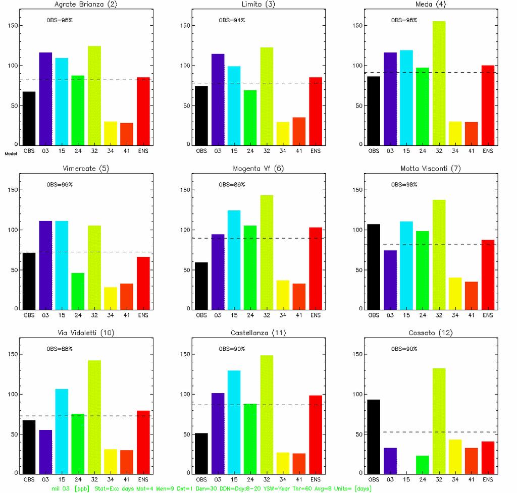
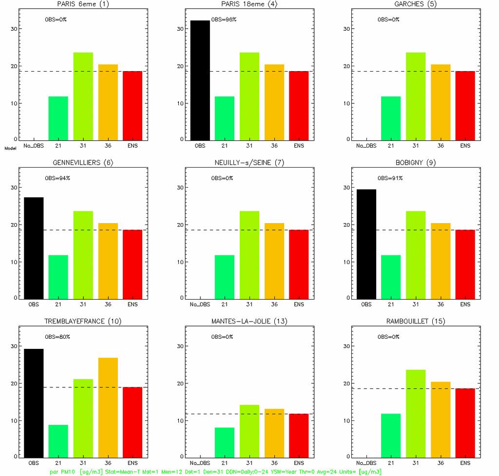
21 5 Analysis of the model output C. Cuvelier, P. Thunis In the following figures a comparison is made between the results of the fine-scale models (Models 03, 15, 24, 32, 34, 41 and the corresponding Ensemble) and the coarse scale models (Models 21, 25, 31, 36 and the corresponding Ensemble). Observations are in black. The red colour represents the Ensemble average. For the figures related to validation, the nine monitoring stations (only eight in Prague) have been selected on the basis of their quality of the measurements and on their representativeness. The delta results are visualised for nine urban locations with the middle-point in the centre of the city. Ozone is given in ppb, PM is given in µg/m Mean summer (April-September) ozone (cf. Figure 5.1) For the cities of Berlin and Paris differences between coarse and fine resolution are relatively limited, and are restricted to the city-centre stations where some models predict large differences related to their spatial resolution (for example Model 24 and 25 in Berlin-Neukölln). In Prague and Milan the differences however are much larger between coarse and fine scale. The variability among the finescale models for these two cities is quite high. This can reach a factor of two for some stations. 5.2 Ozone exceedance days (60 ppb, 8hr average) (cf. Figure 5.2) For Berlin the Ensemble for both coarse and fine scale models generally under-estimate the number of exceedance days with respect to observation. The coarse models slightly tend to predict larger values than the fine-scale models. However for Paris the Ensemble generally overestimates the observed values, where large values are reported for Model 15. Model 25 reports systematically the smallest number of exceedance days. For Prague some models show zero exceedance, but the validation is difficult to make because of a lack of observations at some of the stations. 5.3 Taylor diagram for mean summer ozone (cf. Figure 5.3) In the Taylor diagrams three statistical indicators are visualised: Standard deviation (Stddev, distance to the origin), correlation coefficient (corr_coef, angular distance from the top counting clockwise) and the Centred Root Mean Square error (distance from any model marker to the observation marker as indicated by the black cross in the x-axis). In these diagrams each model marker is representative of all 9 stations previously mentioned. The correlation of all models in all cities ranges from 0.5 to 17

22 0.65. The standard deviation of the measurements is larger in Milan than in other cities and models exhibit difficulties in capturing these standard deviations as is indicated by the wider spread of the model predictions in this city. In other cities, however, all model results are grouped in a narrow region, which proves that they better capture the observational variability. In general, there is no significant difference between the coarse-scale models (indicated by a square symbol) and the finescale models (indicated by the cross symbol). 5.4 Annual mean PM 10 (cf. Figure 5.4) It is more difficult to draw conclusions on the models ability to predict PM 10 since few observations are available in this study. In general the fine-scale models slightly underestimate the observations but are closer to them than the coarse-scale models which also underpredict the observations. There seems to be a problem with Model 31 and 32 in Milan with a strong overestimation of the observed concentration. In Prague the same is true for Model 32 whereas its coarse version (Model 31) is in quite good agreement with the observations. Observations are much higher in Milan than in other cities and the fine-scale models show a larger variability in this city. 5.5 Taylor diagram: Annual mean PM 10 (cf. Figure 5.5) The correlation coefficient for the cities of Berlin and Paris is around 0.6, whereas it is around 0.4 for Milan and Prague. As for ozone, the standard deviation is much larger for Milan, and all models for this city significantly underestimate the standard deviation. From these diagrams Milan appears to be the city where models show a large variability in their predictions. This could be due to the specific geographic location of this city as well as to the general climate conditions. 5.6 Delta (CLE-2000) mean summer ozone (cf. Figure 5.6) All coarse-scale models predict a reduction in the mean summer ozone concentration for the CLE scenario compared to 2000, with the single exception of Model 31 in Prague. The fine-scale models generally agree with a reduction in the cities of Paris and Milan, whereas for Prague and Berlin most fine-scale models predict an increase of mean ozone concentrations. The Ensemble reductions for the fine-scale and the coarse-scale are comparable for Paris. For Milan the coarse-scale Ensemble predicts a larger decrease than the corresponding fine-scale. 18

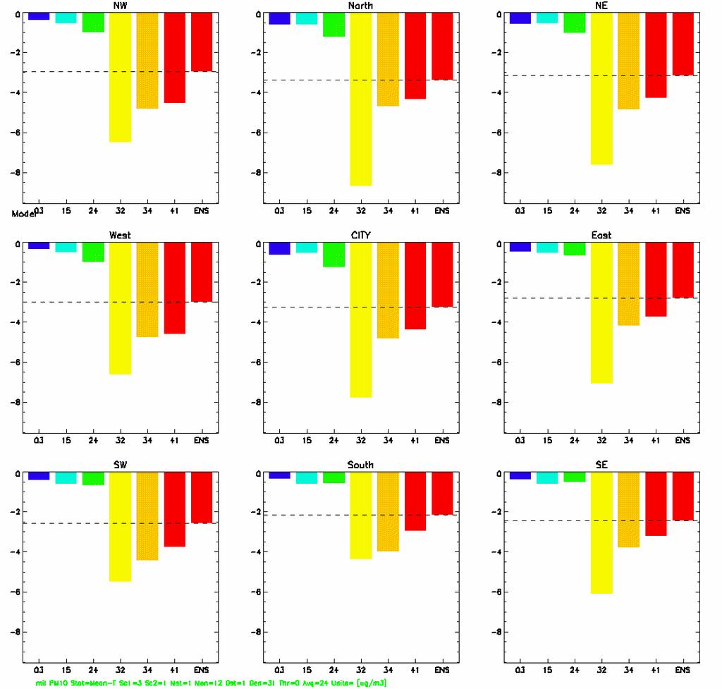
23 5.7 Delta (MFR-CLE) mean summer ozone (cf. Figure 5.7) The differences between CLE-to-MFR reduction and 2000-to-CLE reduction are of the same order of magnitude for Berlin and Prague, but are more significant for 2000-to-CLE in Paris and Milan. Except for Berlin where the majority of the fine-scale models predict a decrease of ozone concentration, the response of these fine-scale models shows some variability in the other cities. Coarse-scale models generally predict a decrease except in Paris where the situation is not so clear. 5.8 Delta (CLE-2000) annual mean PM 10 (cf. Figure 5.8) All models in each city predict a decrease in PM 10 levels. The decreases predicted in Milan (20 µg/m 3 ) are approximately 2 to 3 times larger than for the three other cities. The fine-scale models tend to predict more pronounced decreases than the coarse-scale models. Models 31 and 32 seem to be outliers for the city of Milan. If we exclude the outliers, the models show a consistent behaviour in their response to the 2000-to-CLE emission reduction. Note that Model 24 did not deliver results for the 2000 scenario for Prague, and model 25 not for the 2000 scenario in Paris. 5.9 Delta (MFR-CLE) annual mean PM 10 (cf. Figure 5.9) The conclusions drawn for point 5.8 remain valid for the CLE-to-MFR scenario, except that the reductions are now significantly smaller than for 2000-to-CLE. They are about 1 µg/m 3 for Berlin, Paris and Prague, and about 3 µg/m 3 for Milan. Models 31 and 32 systematically produce for all cities a larger delta than the other models City-overview: Mean summer daytime ozone (cf. Figure 5.10) In this type of figure one can visualise the comparison between the Ensemble models for the fine and the coarse scales in the 4 cities. The Ensembles are constructed by calculating for each city the indicator on the average of the model results based on their values in an area which is representative of the city high-population area (approximately 50 x 50 km 2 ). For the base case (2000) the Ensemble-fine is for all cities predicting lower daytime ozone mean levels with the differences being the largest in Milan (6 ppb). The Ensemble-coarse predicts larger reductions for the CLE scenario compared to the Ensemble-fine (CLE-2000). This remains the same for the NO x -MFR (i.e. MFR1). The VOC-MFR (i.e. MFR2) responses are very similar for the Ensemble-fine and Ensemble-coarse. For the Ensemble-fine results, the three lower figures provide an idea of the impact of MFR emission-reductions applied only on the city area, while keeping the boundary conditions at CLE levels. 19

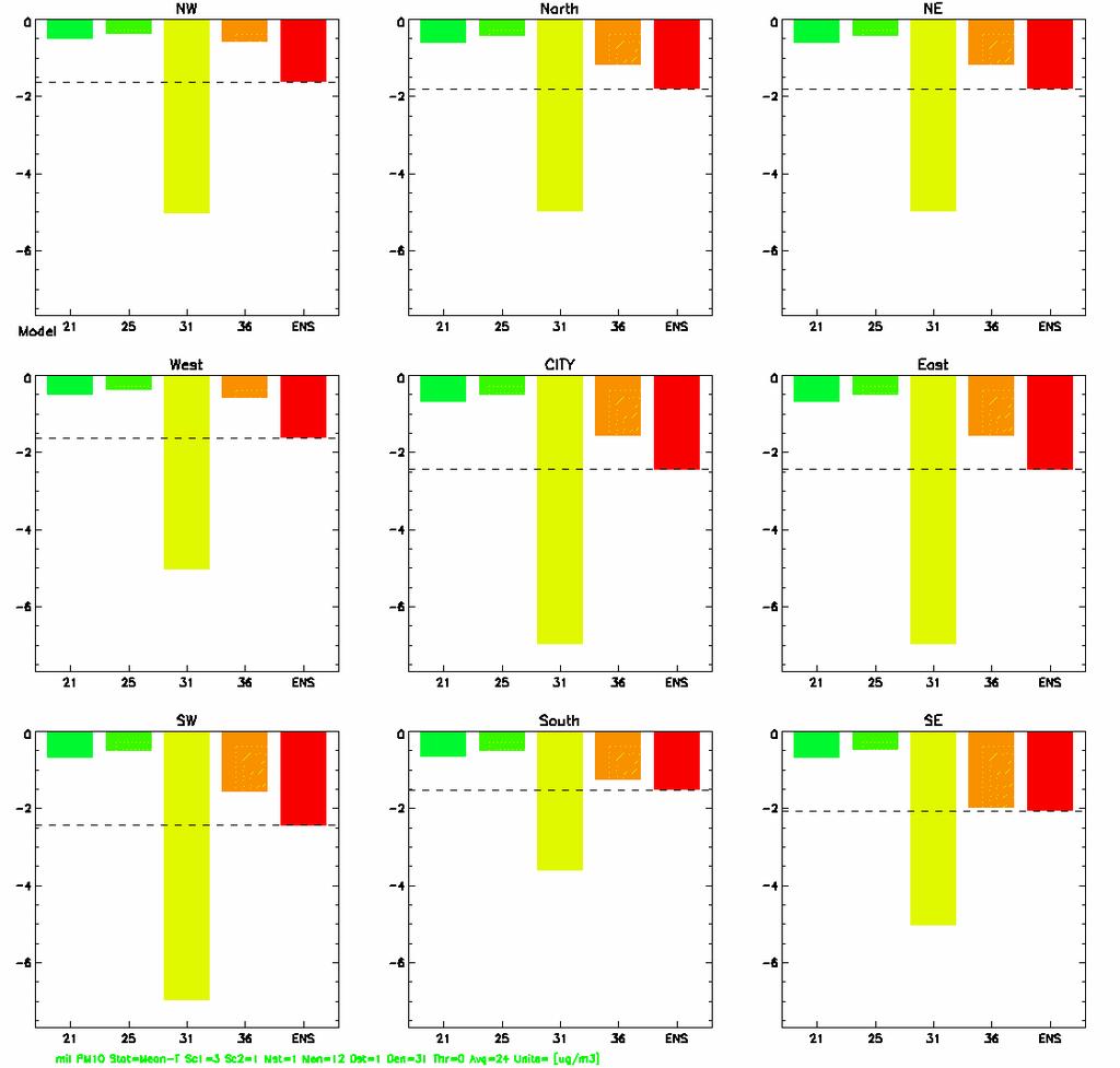
24 From these figures it appears that a NO x reduction limited to the city-area is counter-productive, whereas the VOC reduction is effective both at regional and at city scale. However, it should be noted that the differences are only significant for the city of Milan. The combination of measures taken both at the regional and local scale (i.e. the ^ MFR figures) are more effective than measures limited to the local scale (^ CLE) City-overview: SOMO35 indicator (cf. Figure 5.11) The SOMO35 indicator proposed by WHO during the last meeting of the Task Force on Health in Bonn (May 2004) is defined as the sum over the summer period of the maxima of the daily 8-hr running average ozone concentration in excess of 35 ppb. The conclusions related to this indicator are similar to those valid for the mean summer daytime ozone (Section 5.10) City-overview: Annual mean PM 10 (cf. Figure 5.12) For the base case (2000) the Ensemble-fine is for all cities predicting higher mean PM 10 levels. The Ensemble-coarse predicts smaller reductions for the CLE scenario compared to the Ensemble-fine (CLE-2000). The NO x -MFR (i.e. MFR1 which includes PPM) and VOC-MFR (i.e. MFR2) responses are very similar for the Ensemble-fine and Ensemble-coarse and are approximately a factor of two smaller than for the CLE-2000 reductions. From these figures it appears that both the NO x -PPM (MFR1) and VOC (MFR2) reductions limited to the city-area are effective. Strangely enough in Milan, the combination of measures taken both at the regional and local scale (i.e. the ^MFR figures) are more effective than measures limited to the local scale (^ CLE). This could be due to the behaviour of Model 31 and 32 in this city. For the other three cities about half of the improvement is coming from local measures, the other half being attributed to regional measures City-overview: Annual mean PM 2.5 (cf. Figure 5.13) Similar remarks hold as in the case of PM 10 (Section 5.12). 20

25 BERLIN Figure 5.1:: Mean Summer (April-September) Ozone Fine-scale Coarse-scale PARIS Fine-scale Coarse-scale 21

26 Figure 5.1 (cont.) PRAGUE Fine-scale Coarse-scale MILAN Fine-scale Coarse-scale 22

27 Figure 5.2: Ozone exceedence days (60 ppb, 8hr) BERLIN Fine-scale Coarse-scale PARIS Fine-scale Coarse-scale 23

28 PRAGUE Figure 5.2 (cont.) Fine-scale Coarse-scale MILAN Fine-scale Coarse-scale 24

29 Figure 5.3: Taylor diagram for mean summer ozone Fine-scale and coarse-scale models 25

30 Figure 5.4: Annual mean PM10 BERLIN Fine-scale Coarse-scale PARIS Fine-scale Coarse-scale 26

31 Figure 5.4 (cont.) PRAGUE Fine-scale Coarse-scale MILAN Fine-scale Coarse-scale 27

32 Figure 5.5: Taylor diagram: Annual mean PM10 Fine-scale and coarse-scale models 28

33 Figure 5.6:: Delta (CLE-2000) mean summer ozone BERLIN Fine-scale Coarse-scale PARIS Fine-scale Coarse-scale 29

34 Figure 5.6 (cont.) PRAGUE Fine-scale Coarse-scale MILAN Fine-scale Coarse-scale 30

35 Figure 5.7: Delta (MFR-CLE) mean summer ozone BERLIN Fine-scale Coarse-scale PARIS Fine-scale Coarse-scale 31

36 Figure 5.7 (cont.) PRAGUE Fine-scale Coarse-scale MILAN Fine-scale Coarse-scale 32

37 Figure 5.8: Delta (CLE-2000) annual mean PM10 BERLIN Fine-scale Coarse-scale PARIS Fine-scale Coarse-scale 33

38 Figure 5.8 (cont.) PRAGUE Fine-scale Coarse-scale MILAN Fine-scale Coarse-scale 34

39 Figure 5.9: Delta (MFR-CLE) annual mean PM10 BERLIN Fine-scale Coarse-scale PARIS Fine-scale Coarse-scale 35

40 Figure 5.9 (cont.) PRAGUE Fine-scale Coarse-scale MILAN Fine-scale Coarse-scale 36

41 Figure 5.10: City-overview: Mean summer daytime ozone Note: MFR1-CLE ^ MFR1 = MFR for NO x, SO 2, PPM2.5 and PPMc, and CLE for others (with boundary conditions kept at MFR1) MFR2-CLE ^ MFR2 = MFR for VOC, CO and NH 3, and CLE for others (with boundary conditions kept at MFR2) MFR-CLE ^ MFR = MFR for all pollutants (with boundary conditions kept at MFR) MFR1-CLE ^ CLE = MFR for NO x, SO 2, PPM2.5 and PPMc, and CLE for others (with boundary conditions kept at CLE) MFR2-CLE ^ CLE = MFR for VOC, CO and NH 3, and CLE for others (with boundary conditions kept at CLE) MFR-CLE ^ CLE = MFR for all pollutants (with boundary conditions kept at CLE) 37

42 Figure 5.11: City-overview: SOMO35 indicator 38

43 Figure 5.12: City-overview yearly mean PM10 39

44 Figure 5.13: City-overview: Annual mean PM2.5 40

45 6 Functional relationships to estimate urban air quality C. Heyes, L. White, M. Amann, W. Schöpp It is one of the major objectives of the City-Delta project to develop functional relationships that allow calculating health-relevant metrics of urban air quality in the context of the Europe-wide integrated assessment conducted with the RAINS model. For PM2.5, such relationships should determine urban background concentrations of PM2.5 as a function of grid average concentration as computed by a regional-scale dispersion model, emission densities in a city, which vary inter alia with emission control scenarios, and some topographic and meteorological parameters that reflect city-specific dispersion characteristics. To connect with the determinants of health impact methodologies (i.e., urban background concentrations), such functional relationships should quantify changes in long-term metrics of urban background of PM2.5 and ozone, rather than short-term peak concentrations or hot spots such as street canyons. 6.1 Analysis of observational data To complement the analysis of the City-Delta model intercomparison, which aimed at the understanding of responses of urban air quality towards changes in emissions based on model analyses, an assessment was carried out for observational data. This analysis is based on the concept supported by the findings of City-Delta that a large fraction of PM 2.5 in urban background air originates from long-range transport. The data processing and analysis have been largely determined by practical considerations such as data availability and the quality and accessibility of the relevant data documentation. Investigation has concentrated on the cities of London and Berlin, both of which are represented in the City-Delta project with data available for In addition, it proved to be relatively straightforward to obtain London PM emissions and measurement data for Data Sources The primary PM emission inventory provided to City-Delta for London gives PM 10 emission estimates for 1999 on a 2*2 km grid for both ground-level sources and stacks. Monitoring data are available for 1999 from nine sites, eight of which provide PM 10 concentrations, and two PM 2.5. The Berlin emission inventory provides estimates of PM 10 emissions for a number of source sectors with a spatial resolution of longitude * latitude. Emissions of PM 2.5 are estimated as a sector-dependent fraction of PM 10. The Berlin emission inventories are applicable to years between 1996 and 1999, depending on source sector and origin. Measurements of PM 10 from 41

46 1999 for three Berlin sites two urban, one rural - are available from City-Delta. Additional PM 10 measurement data for the Berlin area for 1999, 2000 and 2001 were obtained from the Airbase measurement database. The UK National Atmospheric Emissions Inventory website ( provides information on the UK emissions of a wide range of pollutants including PM 10. Gridded PM 10 emissions covering the whole of the UK with a spatial resolution of 1*1 km are available for each CORINAIR SNAP1 source sector for the year In the present study, most attention has been given initially to the road transport sector and total area source PM 10 emissions. The UK National Air Quality Information Archive ( contains extensive sets of UK measurements of air quality for periods from 1960 to the present, involving more than 1500 monitoring sites. Hourly measurements of PM 10 concentrations have been made at more than 60 sites across the UK. Results from these sites for 2001 to be consistent with the available emissions data have been obtained for use in this study Results Measurement data rather than model results have been used for these investigations. Annual average concentration values have been calculated; no use has yet been made of greater temporal resolution of the typically hourly concentration measurements available. To date, the study has focused on PM 10 rather than directly on PM 2.5. This is because data on PM 10 is, currently, much more widely available than PM 2.5 data, although the finer fraction is acknowledged to be more relevant to impacts on human health. The aim of these preliminary analyses has been to investigate how measured PM concentrations within urban areas depend on the local PM emission density. This relationship should be examined to establish whether it is better expressed in terms of total PM emissions or as a function of the PM emissions from a specific source sector, such as road transport. Where a clear relationship exists, the most appropriate spatial resolution for the urban emissions needs to be determined London Analysis of monitoring data shows a clear relation between the magnitude of the urban signal and the emission density within the city. An example for London finds a rather consistent linear relation between observed annual mean PM 10 levels at the various urban background monitoring stations and the primary PM 10 emission densities (from road transport) in the 5*5 km box around each measurement site (Figure 6.1). This figure is based on concentration measurements and emission estimates for London for the year It makes use of PM 10 data rather than directly PM 2.5 because of the scarcity of available PM 2.5 measurements. Although it must be remembered that this is a 42

47 preliminary result for one location for one year, it would suggest not only that there is a reasonably good correlation between annual average PM 10 concentrations at urban sites and the local road traffic emissions of PM 10, but also that the urban increment is not a large proportion of the measured PM 10 concentration at urban background sites. For the London example shown here for 2001, the urban increment constitutes at most 27 percent of the measured urban background PM 10 concentration. PM 10 concentration as a function of emission density, primary PM 10 from UK road transport (2001) [PM 10], ug m Roadside sites Urban sites Rural sites PM 10 emission density, t km -2 yr -1 5 km x 5 km Figure 6.1: Relation between measured PM 10 concentrations within London and the emission density of PM 10 from road transport. Both the measurement data and the PM 10 emission inventory are for the year The example shown in Figure 6.1 used the emission density of PM 10 emissions from road transport calculated over the 5*5 km grid cell in which each measurement station is located. Figure 6.2 provides a comparison of the relationships found for total area source PM 10 emissions averaged over different grid areas. Correlations appear to improve if emission densities are averaged over a larger area than 1*1 km; in this case, 5*5 km gives a better result for the urban background sites than 1*1, 3*3 or 9*9 km. Figure 6.3 shows the corresponding comparison of averaging area if only emissions from road transport are considered. As a sideline, it is interesting to note that linear relations between observed annual mean PM 10 levels and emission densities also emerge for roadside sites, though obviously with a steeper slope. 43

48 44

49 y = x R 2 = [PM 10], µg m [PM 10], µg m y = x R 2 = y = x R 2 = PM 10 emission density, t km -2 yr -1 1 km x 1 km PM 10 emission density, t km -2 yr -1 3 km x 3 km y = x R 2 = y = x R 2 = [PM 10], µg m [PM 10], µg m y = x R 2 = y = x R 2 = PM 10 emission density, t km -2 yr -1 5 km x 5 km PM 10 emission density, t km -2 yr -1 9 km x 9 km Rural sites Urban sites Roadside sites Figure 6.2: Relation between measured PM 10 concentrations within London and the emission density of PM 10 from all source sectors. Both the measurement data and the PM 10 emission inventory are for the year The different panels show the effect of averaging the PM 10 emissions over different grid sizes: 1*1 km, 3*3 km, 5*5 km or 9*9 km. 45

50 y = x R 2 = [PM 10], µg m [PM 10], µg m y = x R 2 = y = x R 2 = PM 10 emission density, t km -2 yr -1 1 km x 1 km PM 10 emission density, t km -2 yr -1 3 km x 3 km y = 5.897x R 2 = y = x R 2 = [PM 10], µg m [PM 10], µg m y = x R 2 = y = x R 2 = PM 10 emission density, t km -2 yr -1 5 km x 5 km PM 10 emission density, t km -2 yr -1 9 km x 9 km Rural sites Urban sites Roadside sites Figure 6.3: Relation between measured PM 10 concentrations within London and the emission density of PM 10 from road transport (SNAP1 sector 7). Both the measurement data and the PM 10 emission inventory are for the year The different panels show the effect of averaging the PM 10 emissions over different grid sizes: 1*1 km, 3*3 km, 5*5 km or 9*9 km. The previous figures examined the urban signal within London itself and suggest a reasonably good correlation with PM 10 emission density for measurement sites within London. It is interesting to see whether a similar picture emerges for the whole of the UK or whether the spatial variation in rural 46

51 background PM 10 concentrations masks the trend with urban emission density. Figure 6.4 shows the 2001 annual average PM 10 concentrations at all the available UK monitoring sites as a function of the emission density of PM 10 from UK road transport [PM 10], g m PM 10 emission density, t km -2 yr -1 9 km x 9 km Rural sites Urban sites Roadside sites Figure 6.4: Relation between measured PM 10 concentrations in the UK and the emission density of PM 10 from road transport (SNAP1 sector 7). Both the measurement data and the PM 10 emission inventory are for the year Although a general trend is apparent in Figure 6.4, the data appear too scattered to allow a satisfactory functional relationship to be developed for an area as large as the UK. Data from smaller areas, viz., 200*200 km and 100*100 km, based on the rural monitoring site closest to London, are shown in Figure 6.5. The correlation between measured PM 10 concentrations and the 47

52 emission density of PM 10 from road transport is seen to improve as the area investigated is reduced. The measurement station density is, however, insufficient to allow extending this investigation to grid areas of 50*50 km and smaller y = x R 2 = y = x R 2 = [PM 10], g m [PM 10], g m y = x R 2 = y = x R 2 = PM 10 emission density, t km -2 yr -1 9 km x 9 km PM 10 emission density, t km -2 yr -1 9 km x 9 km Rural sites Urban sites Roadside sites Figure 6.5: Relation between measured PM 10 concentrations and the emission density of PM 10 from road transport (SNAP1 sector 7) in the London area. Both the measurement data and the PM 10 emission inventory are for the year The panel on the left shows data for an area of 200*200 km; the right-hand figure covers a 100*100 km area. 48

53 Berlin Initial analysis of the City-Delta data for Berlin for 1999 generally supports the preliminary findings for London. Figure 6.6 shows the relation between measured PM 10 concentrations within Berlin and the emission density of PM 10 from road transport (upper row) and all area sources (lower row) for 1999 data. Figure 6.7 and Figure 6.8 provide further examples of the PM 10 concentration/emission density relationship using measurements from 2000 and The use of Berlin measurement data for the years 2000 (Figure 6.7) and 2001 (Figure 6.8) has the advantage of providing a greater number of data points for the analysis but with the drawback of an implicit assumption that the PM 10 emission densities in 2000 and 2001 are similar to those in The example plots for Berlin examine the urban PM 10 signal using different PM 10 source categories (road transport, road transport + domestic combustion, or all area sources), with the emission densities averaged over a number of different grid areas. On the basis of the results displayed here, it is not possible to identify unequivocally which combination of source sector and averaging area provides the best fit. For Berlin, it seems that each of the combinations examined would give a reasonable basis for a functional relationship. 49

54 [PM 10], g m y = x R 2 = [PM 10], µg m y = x R 2 = PM10 emission density, t km -2 yr -1 1 cell x 1 cell PM10 emission density, t km -2 yr -1 5 cells x 5 cells [PM 10], µg m y = x R 2 = [PM 10], µg m y = 2.297x R 2 = PM10 emission density, t km -2 yr -1 1 cell x 1 cell PM10 emission density, t km -2 yr -1 5 cells x 5 cells Rural sites Urban sites Roadside sites Figure 6.6: Relation between measured PM 10 concentrations within Berlin and the emission density of PM 10 from road transport (upper row) and all area sources (lower row). Both the measurement data and the PM 10 emission inventory are for the year The different panels show the effect of averaging the PM 10 emissions over different numbers of grid cells. 50

55 [PM 10], g m y = x R 2 = [PM 10], g m y = 4.94x R 2 = PM 10 emission density, t km -2 yr -1 1 cell x 1 cell PM 10 emission density, t km -2 yr -1 3 cells x 3 cells [PM 10], g m y = 2.565x R 2 = [PM 10], g m y = x R 2 = PM 10 emission density, t km -2 yr -1 1 cell x 1 cell PM 10 emission density, t km -2 yr -1 3 cells x 3 cells Rural sites Urban sites Roadside sites Figure 6.7: Relation between measured PM 10 concentrations within Berlin and the emission density of PM 10 from road transport + domestic sources (upper row) and all area sources (lower row). The measurement data in this figure are for the year 2000, the PM 10 emission inventory is for The different panels show the effect of averaging the PM 10 emissions over different numbers of grid cells. 51

56 [PM 10], g m y = x R 2 = [PM 10], g m y = 5.402x R 2 = PM 10 emission density, t km -2 yr -1 1 cell x 1 cell PM 10 emission density, t km -2 yr -1 5 cells x 5 cells [PM 10], g m y = x R 2 = [PM 10], g m y = x R 2 = PM 10 emission density, t km -2 yr -1 1 cell x 1 cell PM 10 emission density, t km -2 yr -1 5 cells x 5 cells Rural sites Urban sites Roadside sites Figure 6.8: Relation between measured PM 10 concentrations within Berlin and the emission density of PM 10 from road transport (upper row) and road transport + domestic sources (lower row). The measurement data in this figure are for the year 2001, the PM 10 emission inventory is for The different panels show the effect of averaging the PM 10 emissions over different numbers of grid cells. 52

57 6.2 Analysis of model results Analysis of measurement data in the previous section indicates a clear and possibly simple relationship between the primary PM concentration and the emission density of low level primary PM emissions in a city. As concluded above, such a relationship can be identified from monitoring data between the urban increment in ambient PM concentrations (compared to a rural background station) and urban emission densities. For the purpose of introducing urban air quality into the RAINS model, such relationships should quantify the difference between urban background concentrations of PM2.5, which are considered as the driving force for the health impact assessment, and the grid average (50*50 km 2 ) PM2.5 concentration as computed by the regional-scale dispersion model. The regional dispersion model includes the emissions of a city within the grid cell and calculates the resulting grid-average PM2.5 concentrations, in principle by assuming the urban emissions uniformly distributed over the entire grid cell. To compensate for this effect (i.e., to reflect that the regional scale model already includes the urban emissions), the analysis relates the increase in PM2.5 concentrations to the differences between urban (local) and the grid-average emission densities. For this purpose, the results from the City-Delta model calculations were analyzed to identify the differences between local sub-grid (C 5x5km ) and grid-average (C Average 50x50km ) PM2.5 concentrations and the difference between local (sub-grid) (E 5x5km ) and grid-average (E Average 50x50km ) emission densities of low level emission sources: C 5x5km -C Average 50x50km and E 5x5km -E Average 50x50km where: C 5x5km -C Average 50x50km is the difference in concentration between any given 5x5km grid in the 50x50km domain (centred on the city) and the average concentration of all 5x5 grids contained in the 50x50km domain E 5x5km -E Average 50x50km is the difference in emission density (t/km 2 ) between any given 5x5km grid in the 50x50km domain (centred on the city) and the average emission density of all 5x5 grids contained in the 50x50km domain These relationships were examined for all modelling results based on the City-Delta model ensemble from each of the three scenarios (Base 2000, 2010CLE and 2020MFR), for the four City- Delta cities (Berlin, Paris, Milano and Prague). Results are displayed in Figure 6.9 to Figure Local emission densities were determined for low level sources only, taking into account emissions from the domestic and transport sectors and, in absence of more detailed information, assuming half of the industrial emissions to be emitted from low sources. 53

58 8 Difference between sub-grid and grid-average PM2.5 concentration (micrograms/m 3 ) Difference between sub-grid and grid-average emission density (t/km 2 ) Base case CLE MFR Figure 6.9: Sub-grid variations in annual mean PM2.5 concentrations versus sub-grid variations in emission densities of low sources, for all 5*5 km2 grid cells in the Berlin City-Delta model domain, for the base case and the CLE and MFR scenarios, as computed by the City-Delta model ensemble Table 6.1: Slopes and correlation coefficients estimated for the different scenarios for Berlin for the results of the City-Delta model ensemble Slope R 2 Base case CLE case MFR case All cases

59 20 Difference between sub-grid and grid-average PM2.5 concentration (micrograms/m3) Difference between sub-grid and grid-average emission density (t/km2) Base case CLE MFR Figure 6.10: Sub-grid variations in annual mean PM2.5 concentrations versus sub-grid variations in emission densities of low sources, for all 5*5 km2 grid cells in the Milano City-Delta model domain, for the base case and the CLE and MFR scenarios, as computed by the City-Delta model ensemble Table 6.2: Slopes and correlation coefficients estimated for the different scenarios for Milano for the results of the City-Delta model ensemble Slope R 2 Base case CLE case MFR case All cases

60 10 Difference between sub-grid and grid-average PM2.5 concentration (micrograms/m3) Difference between sub-grid and grid-average emission density (t/km2) Base case CLE MFR Figure 6.11: Sub-grid variations in annual mean PM2.5 concentrations versus sub-grid variations in emission densities of low sources, for all 5*5 km2 grid cells in the Paris City-Delta model domain, for the base case and the CLE and MFR scenarios, as computed by the City-Delta model ensemble Table 6.3: Slopes and correlation coefficients estimated for the different scenarios for Paris for the results of the City-Delta model ensemble Slope R 2 Base case CLE case MFR case All cases

61 2 Difference between sub-grid and grid-average PM2.5 concentration (micrograms/m3) Difference between sub-grid and grid-average emission density (t/km2) Base case CLE MFR Figure 6.12: Sub-grid variations in annual mean PM2.5 concentrations versus sub-grid variations in emission densities of low sources, for all 5*5 km2 grid cells in the Prague City-Delta model domain, for the base case and the CLE and MFR scenarios, as computed by the City-Delta model ensemble. Table 6.4: Slopes and correlation coefficients estimated for the different scenarios for Prague for the results of the City-Delta model ensemble Slope R 2 Base case CLE case MFR case All cases The analysis reveals very consistent relationships between local deviations in PM2.5 concentrations from the grid average concentrations and differences in local emission densities. Most strikingly, the slopes of the linear regressions identified for each city appear as rather invariant for the different emission scenarios, suggesting for a given city a robust association between emission density of low level sources and the increment of PM2.5 concentrations almost independent of the absolute level of emissions. If results are approximated by linear regressions, slopes vary for the three considered 57

62 emission scenarios by eight to nine percent for Berlin and Paris and by 15 percent for Milano. For Prague, odd results for the maximum feasible reduction scenario need further analysis. While there are certain variations across cities, these increases can be approximated by linear regressions with correlation coefficients (R 2 ) between 0.60 and 0.80 (with the exception of the maximum feasible case for Prague). The variation in the quality of the fit can be explained by different influences of large point sources on urban air quality for the four cities considered. If there are large point sources within the city domain (e.g., Prague), urban PM concentrations will follow less closely the distribution of emissions from low level sources than in cities without large point source emissions (e.g., Paris). A better representation of the influence of large point source emissions on the air quality of individual European cities would require detailed information about present (and future) emissions of individual large plants, which is, however, at the moment not generally available for all European cities. A third finding is that the slopes of the regressions show considerable differences for the four cities (between 0.22 and 1.65), while urban emission densities are rather comparable. Thus, if results from the four cities are pooled together, additional explanatory variables need to be identified to derive a robust and universally applicable functional relationship. As an exploratory analysis, the slopes obtained from the regression analyses for the four cities were plotted against annual mean wind speeds derived from the meteorological database of the EMEP model for the grid cells in which the cities are located. The hypothesis behind this exercise is that annual mean wind speed should reflect the air exchange of a city, which in turn determines to what extent an urban emission will contribute to ambient concentration in a city before it leaves the city domain. Wind speed in a city is influenced by the synoptic meteorological conditions as well as by the topographic situation of the city, e.g., whether a city is located on flat terrain with good ventilation conditions or in a valley or basin with frequent inversion situations, which inhibit the transport of polluted air out from the city. The initial analysis presented in Figure 6.13 is based on European wind speed data representative for the main conditions of a 50*50 EMEP grid cell for use in long-range dispersion models and thus not necessarily representative for the wind speed within individual cities (some of which are located in valleys, e.g., Prague). However, a general relationship can be detected especially when the wind speeds for the cities were adjusted through interpolation with data from neighbouring EMEP grid cells (blue dots in Figure 6.13). Such adjustment recognizes that the footprint of the EMEP grid does not match the foot print of the 50x50km domain of the fine scale modelling (centred on the city) that was used to develop the individual city slopes. In no case was the wind speed adjusted more than 15 percent. Obviously, the analysis presented in this figure has to be considered as preliminary, since it is only based on data for four cities and relies on large-scale wind speed data. 58

63 However, until further data on local wind speeds become available, the exploratory analysis applies the adjusted relationships for the further analysis. Figure 2: Slope of Individual City "Delta PM primary Concentration Against Delta PM primary Emission Density" vs EMEP Wind Speed in City Grid 2.00 PM2.5 Linear (PM2.5) PM2.5 Unadjusted Wind Linear (PM2.5 Unadjusted Wind) Slope delta µg/m3 vs delta t(pm10)/km y = x R 2 = y = x R 2 = EMEP Wind Speed m/s Figure 6.13: Slopes of urban increments in PM concentrations versus the annual mean wind speed extracted from the EMEP meteorological data for the 50*50 km grid cell in which the city is located 6.3 Functional relationships for the RAINS model With the relationships identified above, it becomes possible to estimate urban background concentrations of PM2.5 in the RAINS model. This assessment starts from the grid average PM2.5 concentration estimated by the regional-scale EMEP dispersion model and adjusts these values by urban emission densities and urban wind speed data: 59

64 PM sub-grid = (ED sub-grid - ED EMEP ) * (k1 - k2*v wind ) Equation 6.1 with PM sub-grid.. Difference in PM concentration between sub-grid (urban/rural) area and average of the EMEP grid cell ED x Emission density for low sources (x=urban/rural/emep grid average) V wind Annual mean wind speed k1, k2 Parameters derived from the City-Delta ensemble model Emission densities are readily available for the EMEP grid cells as they establish one input to the EMEP dispersion model calculations, but due to the lack of urban emission inventories for most of the European cities they are generally unavailable for individual cities. Thus, the RAINS model calculates urban emission densities (for a given emission control scenario) based on the fundamental assumption that the spatial distribution of low level sources follows to a large extent the population densities: ED sub-grid = E sub-grid / A sub-grid = Equation 6.2 = E EMEP * (P sub-grid / P EMEP ) / A sub-grid = = E EMEP * (P sub-grid / P EMEP ) * (A EMEP / A EMEP ) / A sub-grid = = ED EMEP * (PD sub-grid / PD EMEP ) with E x Emissions (x=urban/rural/emep grid average) P x Population (x=urban/rural/emep grid average) PD x Population density (x=urban/rural/emep grid average) A x Area (x=urban/rural/average over EMEP grid cell). With this relation, the sub-grid emission density in Equation 6.1 can be expressed as ED sub-grid = ED EMEP * (PD sub-grid / PD EMEP ), 6.3 Equation so that Equation 6.1 emerges as PM sub-grid = (ED sub-grid ED EMEP ) * (k1 - k2*v wind )= = (ED EMEP * (PD sub-grid / PD EMEP ) ED EMEP ) * (k1 - k2*v wind ) = = ED EMEP * (PD sub-grid / PD EMEP 1) * (k1 - k2*v wind ) Equation

65 Thus, calculation of urban emission densities, while scenario-specific, requires the following input data: Emission densities of low level sources in an EMEP cell (for a given emission control scenario) Population densities in the urban and rural areas of an EMEP grid cell Annual mean wind speed in an EMEP grid cell or eventually within the city. With this, Equation 6.1 to compute the urban increment of PM turns into the following formulation, which can be readily included in the RAINS model: PM sub-grid = ED EMEP * (PD sub-grid / PD EMEP 1) * (k1 - k2*v wind ) Equation 6.5 This formulation takes the gridded sectoral primary PM2.5 emissions for low-level sources from EMEP for 2000 as a starting point (i.e., transport (SNAP7), domestic (SNAP2), and 50 % of industry (SNAP3)) and scales for an emission control scenario the gridded sector emissions of 2000 using the country-wide sectoral change in emissions. 6.4 Input data to the RAINS calculations Equation 6.5 is implemented in the RAINS model to compute the urban increment in PM2.5 concentrations, using additional information on Emission densities for low-level sources, Share of urban population in each EMEP grid cell Annual mean wind speeds. Emission densities of low-level sources for the year 2000 are directly extracted from the emission inventory used as input to the EMEP model, which is available in gridded form distinguishing 11 SNAP sectors. For low level sources in urban areas, emissions of SNAP sector 7 (Transport), SNAP sector 2 (Domestic) and 50 percent of the emissions of SNAP sector 3 (Industry) are considered. For future emission control scenarios, emission data for the year 2000 (Figure 6.14) are scaled at a sectoral level by the changes of sectoral emissions occurring in the country for that scenario. 61

66 Figure 6.14: Density of primary PM2.5 emissions from low-level sources for the year 2000 (in tons/km 2 ) as used as input to the EMEP model calculations 62

67 In addition, RAINS calculations require as a grid-specific input the ratio of urban population densities over the population density of the entire grid cell (PD sub-grid / PD EMEP in Equation 6.5) to reflect situations that emissions are not uniformly distributed within a grid cell, but are concentrated in the urban areas, which might constitute only a small fraction of the entire grid cell area. For large cities, which cover a full 50*50 km 2 grid cell (e.g., London), this ratio turns into one, indicating that there is no sub-grid variation between urban and rural areas within the grid cell. To determine these ratios, population and land use data from the LANDSCAN (2000) database have been used and processed with a geographical information system to derive these grid-specific parameters (Figure 6.15). These ratios are particularly high in small cities surrounded by unpopulated area. 63

68 Figure 6.15: Ratio of urban population densities over the population density of the entire grid cell (PD sub-grid / PD EMEP in Equation 6.5) As a third element, Equation 6.5 considers wind speed to determine the urban increments of PM2.5 concentrations. The present implementation of the functional relationships rely on the wind speed data contained in the EMEP meteorological database, which reflect large scale grid-average wind conditions that are appropriate for modelling of the atmospheric long-range transport. As discussed above, this data set might not be representative for the conditions within urban areas and should be replaced by more appropriate data in the future. 64

69 Figure 6.16: The wind-speed dependent term (k1 - k2*v wind ) in Equation 6.5, based on wind speed data from the EMEP Eulerian model. High values of this term indicate stagnant conditions, low values correspond to high wind speeds. 6.5 Preliminary results With these data, the urban increments to annual mean PM2.5 concentrations in urban areas resulting from urban emissions on top of the concentrations computed by the regional scale (50*50 km 2 ) dispersion calculations have been calculated according to Equation 6.5. As shown in Figure 6.17, large increments occur in Mediterranean and Nordic cities, while increments in central Europe are 65

70 lower. While such large increments in Mediterranean and Nordic cities are confirmed by the sparse observational data, the lower values computed for central Europe, especially for Germany, need further analysis. A number of aspects are of relevance: Some of the large European cities in this region (e.g., London, Paris) extend over one or several entire EMEP grid cells, and are thus (at least in theory) already fully captured by the regional scale model with its 50*50 km 2 resolution. In densely populated areas (e.g., in the Benelux region) there are only low spatial differences in population densities between urban and the surrounding rural areas. Consequently, there is also very little difference in PM2.5 concentration. This is confirmed, e.g., by the Belgian measurements for the twin sites of Gent and Wassemunster as reported in Puteaud et al. (2002). Also PM2.5 measurements in various cities of Northrine-Westfalia (Germany) show very little variation (see The preliminary calculations rely on EMEP grid average wind speeds, which might not be representative for cities, especially when they are located in valleys and basins. While in the northern part of Central Europe high wind speeds dominate at the large scale, the employed data set might miss conditions for individual cities. Work continues to acquire a more appropriate data set for this analysis. Some uncertainty is introduced by the population density related term in Equation 6.5. At present, data are extracted from the LANDSCAN dataset, which derives land use and population data for administrative units. While differences between urban and rural population densities might indeed be small for many German areas, the spatial definitions of the administrative units ( Landkreise ) underlying the data set might dilute existing differences. Further work will be necessary to compile a revised data set with a sharper distinction between urban and rural areas. 66

71 Figure 6.17: The urban increment of PM2.5 (in µg/m 3, annual mean concentrations) calculated with the functional relationship for the year These urban increments are additional to the concentrations computed by the regional scale calculations of the EMEP model using the 50*50 km spatial resolution. To compute total PM2.5 concentrations in urban areas, the urban increment as displayed in Figure 6.17 needs to be complemented by the grid average PM2.5 concentrations as computed by the regional scale EMEP dispersion model (Figure 6.18). It is important to mention that these calculations include the contribution from primary emissions of PM2.5 from anthropogenic sources 67

72 and from secondary inorganic aerosols, but they exclude the contributions from natural emissions and from secondary organic aerosols. As shown in the graph, some of the largest cities (e.g., Paris, Katowicze, Lyon, Marseille, Athens, the London conurbation, etc.) are directly visible in the regional scale calculations, since they extend over entire EMEP grid cells. In such situations, the urban (sub-grid) increment computed by the functional relationships will be low. It is also important to mention that some other large cities (e.g., Berlin), which are more isolated surrounded by areas with relatively low population and emission densities, do neither show up in the regional scale calculations nor in the computations of the urban increment. This is caused by the fact that a number of cities is exactly located at the borderlines of the EMEP grid system and thus fall into two or four EMEP grid cells. The logic of the regional scale calculations considers in such situation only the respective share of emissions in each grid cell and assumes that to be evenly distributed over the entire area. Thus, as is the situation for e.g., Prague, the urban emissions, while located in reality in an area of approximately 15*15 km 2, are smeared out over four grid cells, i.e., over 100*100 km 2 ), and thus are not seen any more for the regional model as a city. The same applies to the functional relationships, which are presently constructed under the assumptions that a city is located in the centre of a 50*50 km 2 grid cell. A further refinement of the methodology will be necessary to address these specific situations in a more accurate way. 68

73 Figure 6.18: Grid-average annual mean PM2.5 concentrations as computed by the EMEP Eulerian model with the 50*50 km2 spatial resolution. This includes contributions to PM2.5 from anthropogenic primary PM emissions and from secondary inorganic aerosols, but does not account for PM2.5 from natural sources and from secondary organic aerosols Comparison with monitoring data To validate the approach, the results obtained from the functional relationships together with the outcome of the regional scale calculations have been compared with monitoring data. Unfortunately, there are very few quality-controlled observations of PM2.5 concentrations available 69