Advanced features of Equilib

Transcription

1 Advanced features of Equilib The Equilib module has many advanced features which are described here. Table of Contents Section 1 Table of Contents Section 2 Target Phases [F],[P],[S] Section 2.1 [F] - Formation target (CaO-SiO 2 ) Section 2.2 [P] - Precipitate target (CaO-SiO 2 and (CaO-SiO 2 -Al 2 O 3 ) Section 2.3 [C] - Composition target (deoxidation of Fe-AlO) Section 3 Phase transitions: CaO-SiO 2 immiscibility (FACT-SLAG) Section 4 Solution properties <1-A>NaCl + <A>KCl Section 5 Include dilute solutions: Section 5.1 Cr in Cu-Fe alloy Section 5.2 Tl 2 O+HfO 2 in Slag Section 6 Limitations and restrictions on the use of dilute components Section 7 Pseudonyms Section 8 Include molar volumes Section 9 Open versus closed system Section 9.1 Desulphurisation of Cu 2 S by air Section 9.2 Deleading of Cu-1%wtPb by argon refining (continued) 1.1

2 Advanced features of Equilib - Table of Contents (continued) Section 10 Section 10.1 Section 10.2 Section 10.3 Section 10.4 Section 11 Section 11.1 Section 11.2 Section 11.3 Section 11.4 Section 11.5 Section 12 Section 13 Section 14 Parameters Menu Dimensions Target limits and Stop/Kill Predominant species Dilute extrapolation, Cut-off, Output mass units Reactants Window Options Combining reactants into one composite chemical species Arbitrary chemical formula (permitting missing species) Mixing mass units - moles, grams, lbs Importing a stream/mixture Reaction table Data Search: gas ions, aqueous species, limited data, CxHy Databases Cooling calculations Equilibrium cooling, Scheil-Gulliver cooling, full annealing of cast alloys Paraequilibrium and minimum Gibbs energy calculations 1.2

3 Target phase options A species or solution phase may be declared as a Target phase. There are several types of target phases: 1. [F] - Formation target phase: the T (P or <A>) is calculated when the species or phase first begins to form. The final T (P, <A>) must not be specified (blank column) and an estimate of the unspecified T (P, <A>) must be entered. 2. [P] - Precipitate target phase: the T (P or <A>) is calculated when another species or phase first starts to precipitate from this phase. The precipitate target phase must be a solution (for example FACT-SLAG or gas phase). The final T (P, <A>) must not be specified (blank column) and an estimate of the unspecified T (P, <A>) must be entered. 3. [C] - Composition target phase: the <A> is calculated for a given solution composition. The final T and P must also be specified and final <A> must not be specified (blank column). 2.0

4 Temperature ( C) Formation target phase The program calculates when this phase first forms (activity = 1, and generally zero mass). One of T, P or alpha must not be specified (i.e. blank) so that Equilib can calculate the limiting T (P or alpha) when the formation target phase first forms. The formation target phase may be a compound species (for example a pure solid or liquid) or a solution phase (gas phase or real solution such as FACT-SLAG) CaO - SiO 2 <A> = 0.35 FactSage 2400 Slag 2200 Slag + CaO(s) Ca 2 SiO 4 (s3) + CaO(s) Slag + Slag#2 T = 1800 C 1600 Slag + Slag + SiO 2 (s6) Ca 3 SiO 5 (s) + CaO(s) Ca 2 SiO 4 (s3) 1400 CaSiO 3 (s2) Ca 2 SiO 4 (s2) + CaO(s) Ca 3 Si 2 O 7 (s) SiO 2 (s4) + CaSiO 3 (s2) SiO 2 (s4) + CaSiO 3 (s) Values of <A> and T used in the following example. CaSiO 3 (s) Ca 2 SiO 4 (s) + CaO(s) Ca 3 Si 2 O 7 (s) SiO 2 (s2) + CaSiO 3 (s) mole fraction SiO

5 Setting a FACT-SLAG formation target at a given composition 1 Right-click on the + column to open the FACT-SLAG extended menu and select F - formation target phase. 2 Enter a value of <A> (0.35) and leave a blank for the value of T(C) in the input boxes of the Final Conditions frame. This activates the Formation Target frame. 3 The Formation Target frame is enabled. Enter an estimate for the value of T(C). Here T(C)= 1000 C. The program will calculate that temperature when FACT-SLAG first starts to form (0 mole)

6 Calculation of the FACT-SLAG formation target at a given composition Note: activity = 1.0 number of moles = 0 for the slag phase (liquid) i.e. FACT-SLAG is just beginning to form. Compositions and quantities of the solid oxides in equilibrium with FACT-SLAG. Value of <A>, X SiO2 =

7 Formation Target phase: specifying the target phase mass In the Menu-Equilib window Formation Target frame, the target phase mass is set to 0.5 mole. Note: The slag-liquid composition is now: X SiO2 = and the temperature has increased to: T = C Value of <A>, X SiO2 =

8 Setting a FACT-SLAG formation target at a given temperature 1 Right-click on the + column to open the FACT-SLAG extended menu and select F formation target phase. 2 Enter a value of T (1800 C) and leave a blank for the value of <A> in the input boxes of the Final Conditions frame. 3 The Formation Target frame is enabled. Enter an estimate of the value of <A>. Here <A> = 0.5. The program will calculate that composition when FACT-SLAG first starts to form (0 mole)

9 Calculation of the FACT-SLAG formation target at a given temperature (1800 C) Note: activity = 1.0 number of moles = 0 for the slag phase (liquid) i.e. FACT-SLAG is just beginning to form. Compositions and quantities of the solid phases in equilibrium (activity =1) with FACT-SLAG. Calculated value of <A> =

10 Temperature ( C) Precipitate target The program calculates when a second phase first starts to precipitate (activity = 1, zero mass) from this target solution phase (activity = 1, 100% mass). One of T, P or alpha must not be specified (i.e. blank) so that Equilib can calculate the limiting T (P or alpha) when the second phase precipitates. The precipitate target phase must be a solution phase for example gas or FACT-SLAG CaO - SiO 2 <A> = 0.35 FactSage 2400 Slag 2200 Slag + CaO(s) Ca 2 SiO 4 (s3) + CaO(s) Slag + Slag#2 T = 1800 C 1600 Slag + Slag + SiO 2 (s6) Ca 3 SiO 5 (s) + CaO(s) Ca 2 SiO 4 (s3) 1400 CaSiO 3 (s2) Ca 2 SiO 4 (s2) + CaO(s) Ca 3 Si 2 O 7 (s) SiO 2 (s4) + CaSiO 3 (s2) SiO 2 (s4) + CaSiO 3 (s) Values of <A> and T used in the following example. CaSiO 3 (s) Ca 2 SiO 4 (s) + CaO(s) Ca 3 Si 2 O 7 (s) SiO 2 (s2) + CaSiO 3 (s) mole fraction SiO

11 Setting a FACT-SLAG precipitate target at a given composition 1 Right-click on the + column to open the FACT-SLAG extended menu and select P precipitate target phase. 2 Enter a value of <A> (0.35) and leave T(C) blank. 3 The Precipitate Target frame is enabled. Enter an estimate of the value of T(C). Here T(C)= 1000 C

12 Calculation of the FACT-SLAG precipitate target at a given composition Equilibrium at C Note: activity = 1.0 number of moles =1 (100%) for the first phase: the slag phase (liquid). First precipitate to deposit from the slag phase activity = 1.0 number of moles = 0. Value of <A>, X SiO2 =

13 1 Right-click on the + column to open the FACT-SLAG Setting a FACT-SLAG precipitate target at a given temperature extended menu and select P precipitate target phase. 2 Enter a value of T (1800 C) and leave <A> blank. 3 The Precipitate Target frame is enabled. Enter an estimate of the value of <A>. Here <A> =

14 Calculation of a FACT-SLAG precipitate target at a given temperature Note: activity = 1.0 number of moles =1 (100%) for the first phase: the slag phase (liquid). First precipitate to deposit from the slag phase activity = 1.0 number of moles = 0. Calculated value of <A>, X SiO2 =

15 Precipitate target phase calculation for a more complex system This is an example of a Slag-liquid precipitate target phase calculation in the CaO-SiO 2 -Al 2 O 3 ternary system. In a precipitate target phase calculation, the temperature (or composition) is calculated when a second phase first starts to form (activity = 1, and zero mole) from the «precipitate target phase». The «precipitate target phase» must be a solution for example, gas, FACT-SLAG, etc. (this differs from the «formation target phase» that can be any type of phase). In this example that temperature is calculated when the first solid precipitate starts to deposit when Slag-liquid (FACT- SLAG) is cooled. Such a calculation is extremely important for example in the pyrometallurgy and glass industries. In principle one could select the equilibrium «transitions» option and execute a normal calculation, but this may lead to lot of unwanted output, especially if the system is complex. Red rimmed dot: for the 1 st example Teal line for <B> = 25% (2 nd example) L+C 2 S+C 3 S C 3 S C 2 S L+C 3 S+C System SiO 2 - CaO - Al 2 O C weight fraction SiO L + C L+C 2 S L L+C 3 S SiO 2 L + S weight fraction Al2O L+CA 6 CaO CA CA 6 2 Al 2 O 3 L+CA 6 +CA 2 weight fraction CaO L + Mullite L+ CA 2 L + A L = Liquid C = CaO A = Al 2 O 3 S = SiO 2 C 2 S = (CaO) 2 (SiO 2 ) C 3 S = (CaO) 3 (SiO 2 ) CA 2 = (CaO)(Al 2 O 3 ) 2 CA 6 = (CaO)(Al 2 O 3 ) 6 Mullite L+A+Mullite L+A+CA

16 Setting a ternary system in the Equilib Reactants Window In the Reactants Window the reactants are <1-A-B> CaO + <A> SiO 2 + <B> Al 2 O 3. This defines a CaO-SiO 2 -Al 2 O 3 ternary system if <A> + <B> is in the range 0 to 1. The use of unit mass (g or lb) will give the compositions in weight %. All data taken from the FACT compound and solution databases

17 Setting the FACT-SLAG precipitate target at a given composition 1 Right-click on the + column to open the FACT-SLAG extended menu and select P precipitate target phase. 2 Enter values for <A> (0.35) and <B> (0.25) (i.e. %wt CaO = 40%, %wt SiO 2 = 35%, %wt Al 2 O 3 = 25%) and leave T(C) blank. 3 The Precipitate Target frame is enabled. Enter an estimate of the value of T(C). Here T(C) = 2000 C. <A> is a variable, <B> is a constant (here, 25 wt.%) that must be defined

18 Precipitate target Results Equilib reports the temperature ( C) where the second phase (Ca 2 Al 2 SiO 7 (s1)) starts to precipitate from the target phase (Slag-liquid). Notes: the composition of the first phase (Slag-liquid) is the same as the input values. activity = 1.0 number of grams = 1 (i.e. 100%) + First precipitate to deposit from the slag phase activity = 1.0 number of grams = 0. Value of <A>, wt% SiO 2 = 35%

19 Performing a composition Precipitate Target calculation As in the previous example on Formation Target calculations, it is possible to perform a composition Precipitate Target calculation on <A> (constant <B> remains unchanged). For example, if in the Menu Window the composition <A> is now unspecified (blank), <B> is still 25% and now the temperature is set to 1600 C, an estimate of <A> is 50%

20 Composition Precipitate Target calculation: Results In the Results Window Equilib now reports the silica (SiO 2 ) composition (<A> = wt.%) at 1600 C where CaO(s1) first starts to precipitate (activity = 1, 0 gram) In the ternary phase diagram at 1600 C (see slide 4.0), there are two liquidus lines intersecting the composition line for which <B> = 25wt.%. One on the CaO-rich side (calculated here) and one on the SiO 2 -rich side

21 Composition Precipitate Target calculation: setting another estimate By setting (in the Menu Window) another estimate for ALPHA <A> on the SiO 2 -rich side, one can calculate the other value of <A> for which a precipitate starts to form. In the Results Window Equilib now reports the silica (SiO 2 ) composition (<A> = wt.%) at 1600 C where mullite Al 6 Si 2 O 13 (s1) first starts to precipitate (activity = 1, 0 gram)

22 Compostion target phase TTD 2.3.0

23 Temperature ( C) Transitions in the CaO-SiO 2 binary phase diagram Liquid phase immiscibility for example X SiO2 = and at 1800 C CaO - SiO 2 FactSage 2400 Slag 2200 Slag + CaO(s) 2000 Ca 2 SiO 4 (s3) + CaO(s) 1800 Slag + Slag# Slag + Slag + SiO 2 (s6) Ca 3 SiO 5 (s) + CaO(s) Ca 2 SiO 4 (s3) CaSiO 3 (s2) + Ca 3 Si 2 O 7 (s) SiO 2 (s4) + CaSiO 3 (s2) 1000 Ca 2 SiO 4 (s2) + CaO(s) SiO 2 (s4) + CaSiO 3 (s) CaSiO 3 (s) Ca 2 SiO 4 (s) + CaO(s) Ca 3 Si 2 O 7 (s) SiO 2 (s2) + CaSiO 3 (s) mole fraction SiO 2 3.1

24 Isothermal phase transitions in the CaO-SiO 2 binary system 1 Binary system <1-A> CaO + <A> SiO 2. 2 Possible products: pure solid oxides liquid Slag (FACT-SLAG) with a possible 2-phase immiscibility (I) 3 <A> = 0.7, 0.75,, 1.0 T ( C) = Select transitions The program will calculate the equilibrium at 1800 C for mole fractions of SiO 2 varying from 0.7 to 1 in increments of 0.05 and will search for all phase transitions. 3.2

25 Step 2 : Products Selection compound species 1 In the Menu-Equilib window Compound species frame, right-click on the pure solids checkbox to open the Species selection window. 17 pure solid oxides 2 Click on Clear, then on Select/Clear and then select all (solid) species containing Oxygen. 3 Press OK to return to the Menu-Equilib window. An asterisk (*) indicates custom selection for the pure solids. 3.3

26 Step 2 : Products Selection solution species 1 In the Menu-Equilib window Solution species frame, right-click on the + column to open the FACT-SLAG extended menu. 2 In the FACT-SLAG extended menu, select option I. 3 The I indicates a possible 2-phase immiscible region. [ I ] - 2-phase Immiscibility: the solution phase may be immiscible. Use this option for FACT-SLAG when SiO 2 > 50%. If the phase is not immiscible the results of the calculation will be OK - the phase will appear twice with the same composition. Note: This option tends to slow down the speed of the calculation - you may wish to try I! (immiscible and dormant) to check if the phase is stable. 3.4

27 Compositions at the two ends of the 1800 C tie-line 2-phase transitions the ends of the 1800 C tie-line. i.e. Equilib reports twophase stability within the composition range: < X SiO2 < and one-phase stability outside this range. 3.5

28 One-phase and two-phase stability at 1800 C Example of two-phase stability at X SiO2 = 0.85 Example of one-phase stability at X SiO2 = 0.75 Slag-liquid#2 is close to forming its activity is In such systems, if option «I» is not selected, the results may be in error even when the second liquid (Slag-liquid#2) is not stable (as in the above example). 3.6

29 Constant composition in the CaO-SiO 2 binary system X SiO2 = 0.35 The program will calculate all phase transitions at X SiO2 = 0.35 in the temperature range 600 to 2600 C. 3.7

30 Transition Temperatures for X SiO2 = 0.35 in CaO-SiO 2 In the Results Window, Equilib reports all phase transitions at <A> = 0.35 within the temperature range 600 to 2600 C. Most transitions report both compositions on each side of the tie-line. Such information is important in complex systems. Transitions at: C, C, C, C. <A> = X SiO2 = 0.35 For example at C: a -Ca 2 SiO 4 to a-ca 2 SiO 4 3.8

31 Solution Properties: FACT-Salt in the NaCl-KCl binary system 1 The reactants are <1-A> NaCl + <A> KCl i.e. the NaCl-KCl binary system where <A> varies from 0 to 1. 2 The only possible product is the solution phase: Salt-liquid (FACT-SALT) 3 The final conditions The program calculate the equilibrium in Salt-liquid at 850 C for mole fractions of KCl varying from 0 to 1 in increments of Calculate 4.1

32 Solution Properties: opening the window 1 Right-click on the + column to open the FACT-Salt extended menu and select solution properties 1a or point to FACT-SALT and double-click This option lists the common partial and integral solution properties for the phase. The option is only active if the equilibrium has been calculated and the solution phase is stable. 4.2

33 Solution Properties Window and menus Open spreadsheet to view the selected partial properties of the selected phase: FACT-SALT 4.3

34 Solution Properties: Changing Standard States In the solution properties window menu, select Standard States > Change Standard States and click in the + column to select the new standard state. 4.4

35 Solution Properties: Molar Partial Properties Spreadsheet 4.5

36 Solution Properties: Molar Integral Properties Spreadsheet Open spreadsheet to view the selected integral properties of the selected phase: FACT-SALT 4.6

37 Include dilute solution: Cr in Cu-Fe alloy The FACT-CuLQ solution (Cu(liq) alloy) does not contain Cr. This example shows how to create a dilute Henrian solution of Cr and then merge it into the FACT-CuLQ solution phase. 1 Cu Fe Cr that is, Cu may be considered as a solvent and Fe and Cr as solutes

38 Include dilute solution: Cr in Cu-Fe alloy Possible products Possible products at 1200 C and 1 atm: Compound species: pure liquids, pure solids Solution species: FACT-CuLQ Short description of the FACT-CuLQ Solution Phase. It does not contain Cr. Right-click to open the pure liquids Species Window 5.1.1

39 Creating an ideal Henrian solution of Cr(liq) 1 Right-click to open the Cr(liq) extended menu 2 Select Ideal Solution > Ideal solution #1 In an earlier example taken from the Equilib Slide Show Regular Examples (slide 54), the Henrian activity coefficient of Cr(liq) in Cu(liq) was calculated from the binary Cu-Cr phase diagram and reported as: log 10 [g Cr(liq) ] = /T(K) = A/TK + B 3 Enter the values of A and B. Specify New mixing particles P = 1 (this is the default setting), and enter the solution name dilutecr. 4 Press OK 5.1.2

40 Merging the ideal solution dilutecr and FACT-CuLQ 7 Select m - merge dilute solution from > Dilute Solution #1 - dilutecr # denotes species also used in ideal solution 1 and h indicates an henrian activity coefficient 5 Press OK to return to the Menu Window 6 Right-click in the + column of FACT-CuLQ to open its extended menu

41 Calculation including a dilute solution: Cr in Cu-Fe alloy Recalling that the Henrian activity coefficient of Cr(liq) in Cu(liq) is: log 10 [g Cr(liq) ] = /T(K) We have, at 1200 C ( K), g Cr(liq) = The dilute solute (Cr) is merged into the existing FACT-CuLQ solution. Lets calculate the equilibrium and retrieve the calculated value of g Cr(liq) at 1200 C 5.1.4

42 Cr in Cu-Fe alloy Results T = 1200 C X Cr(liq) = Hence, at 1200 C, the calculated activity coefficient is: a C r(liq ) g C r(liq ) X C r(liq ) a Cr(liq) = With the m option you can merge almost any type of dilute solute into an existing real solution

43 Include dilute solution: Tl 2 O and HfO 2 in FACT-Slag The FACT-SLAG (Slag-liquid) solution does not contain the components Tl 2 O and HfO 2. This example shows how to merge Tl 2 O and HfO 2 solutes into a FACT-SLAG containing SiO 2 -CaO-Al 2 O 3 taking into account the «New mixing particles» since HfO 2 dissolves as Hf 4+ and 2 O 2-, and Tl 2 O dissolves as 2 Tl + and O 2-. We wish to create a liquid slag solution which is an equimolar mixture of SiO 2 -CaO- Al 2 O 3 containing small amounts of Tl 2 O and HfO 2. It is assumed that the activity coefficients (defined as g = a/x where a = activity and X = mole fraction) of the dilute constituents are independent of composition. That is, the dilute components obey Henry's Law. Also, for demonstration purposes let us assume that the activity coefficient of HfO 2 at 1000 C in the equimolar mixture is approximately: g HfO2 = 9.0 with respect to its pure solid standard state. Finally, suppose that there is no information on the activity coefficient of Tl 2 O and so ideal solution behavior (g = 1) is assumed for this component. In this case it is necessary to take into account the fact that a liquid slag is an ionic mixture and that Tl 2 O dissociates in solution to form two independent Tl ions. That is, the formula «Tl 2 O» really represents two moles of Tl ions dissolved in the slag. That is, it is actually the component TlO 0.5 which follows ideal solution behaviour

44 Tl 2 O and HfO 2 in FACT-Slag Reactants The reactants are: CaO SiO Al 2 O Tl 2 O HfO 2 The system is an equimolar mixture of CaO, SiO 2 and Al 2 O 3 with Tl 2 O and HfO 2 added as dilute components

45 Tl 2 O and HfO 2 in FACT-Slag Possible products Possible products at 1000 C and 1 atm: Solution species: FACT-SLAG Compound species: ideal gas Short description of the FACT-Slag Solution Phase. It does not contain Tl 2 O nor HfO 2. Right-click to open the pure solids Species Window 5.2.2

46 Creating an ideal Henrian solution of HfO 2 (s) 1 Right-click to open the HfO 2 (s2) extended menu 2 Select Ideal Solution > Ideal solution #

47 Creating an ideal Henrian solution of HfO 2 (s) setting g 3 Enter log 10 [g HfO2 (s2)] = /T(K) + 0 in order that g = 9.0 when T = K (1000 C). 4 Specify New mixing particles P = 1 (this is the default setting). 5 Replace the default solution name «Ideal-1» by a new name «DilOxide». 6 Press OK to return to the Solid Species Window. Notes: 1. In general, if g is known at only one temperature, it is better to assume that RT log g = constant than to assume that log g = constant. 2. In this example note that g is the activity coefficient relative to SOLID HfO 2 (s2) as standard state

48 Adding Tl 2 O(l) to the ideal solution # denotes species also used in ideal solution 1 and h indicates an henrian activity coefficient 7 Press OK to return in the Menu Window 8 Right-click to open the pure liquids Species Window 5.2.5

49 Adding Tl 2 O(l) to the ideal solution setting g 9 Right-click to open the Tl 2 O(liq) extended menu 10 Select Ideal Solution > Ideal solution #1 11 Log g is set equal to 0 (i.e. g = 1), Enter A = B = 0 12 Specify New mixing particles P = 2 to indicate that one mole of Tl 2 O dissociates into 2 independent particles (2[Tl + ]) in the oxide solution

50 Henrian activity coefficient, g and new mixing particles, P A dilute solute in an ideal solution may have a Henrian activity coefficient, g, where: log 10 g = A/TK + B You specify A and B, and the number of new mixing particles P. Examples: 1. Solute Sn(s) dissolving in Pb(s) : P = 1 since Sn is a new particle. 2. Solute NaF(liq) dissolving in LiCl(liq) (i.e. Li + and Cl - ): P = 2 since NaF dissolves as new mixing particles Na + and F Solute NaCl(liq) dissolving in LiCl(liq) (i.e. Li + and Cl - ): P = 1 since NaCl dissolves as Na + and Cl - but only Na + is a new particle. 4. Solute S 2 (liq) dissolving in Fe(liq) as S: P = 2. In the present example P = 2 because Tl 2 O dissociates in the slag as: Tl 2 O 2 Tl + + O

51 Merging the ideal Henrian solution DilOxide and FACT-Slag An ideal Henrian solution (DilOxide) of Tl 2 O and HfO 2 has now been created. 13 Press OK to return to the Menu Window 14 Right-click in the + column of FACT-Slag to open its extended menu. 15 Select - merge dilute solution from > Dilute Solution #1 - DilOxide 5.2.8

52 Calculation including a dilute solution: Tl 2 O and HfO 2 in CaO-SiO 2 -Al 2 O 3 slag Click on details to display a summary of the ideal solution data entry. The dilute solution (DilOxide) is merged into the existing FACT-Slag solution

53 Tl 2 O and HfO 2 in CaO-SiO 2 -Al 2 O 3 slag: Results (FACT format) X H fo because Tl 2 O dissociates into two Tl ions and also Al 2 O 3 dissociates into two Al ions: Al 2 O 3 2 Al O 2- Note: This information about Al 2 O 3 is included in the FACT-SLAG database. The calculated activity of HfO 2 (s2) is: a g 9. HfO HfO HfO X Note: If we increase g HfO2, the calculated activity would increase until solid HfO 2 (s) would be calculated to precipitate when its activity = 1.0. If the solubility of HfO 2 were experimentally known for instance, then we could adjust g HfO2 in this way in order to reproduce the measured solubility. That is, a measured solubility limit permits us to determine the value of the Henrian activity coefficient

54 Tl 2 O and HfO 2 in CaO-SiO 2 -Al 2 O 3 slag: Results (ChemSage format) X T lo a The calculated activity of Tl 2 O(liq) is: g X T l O Tl O T l O T l O g X T lo Note: The calculated vapor pressure of Tl gas is atm. If experimental vapor pressure data were available, then one could adjust g Tl2 O in order to reproduce these data. That is, a measured vapor pressure permits one to determine the value of the Henrian activity coefficient

55 Limitations and restrictions of merging dilute solutes into solutions 1. Ions are not permitted as dilute species (ex: Na +, AlClO 3 - in 'dilutecr'). 2. The resulting solution should be dilute in the solute(s) that are merged (ex: in the present case if the resulting solution phase is say >10% Cr then the validity of the results would be in question). 3. Try to avoid species that are already present in the existing database (ex: in the present case avoid adding dilute Fe(liq)). 4. You may create several different ideal Henrian solutions, each with one or more solutes, however: 1. a given solute can only appear in one ideal solution (ex: in the present case Cr(liq) is a solute only in 'Ideal Solution #1 - dilutecr' ). 2. each ideal Henrian solution can be merged only once into one real solution (ex: in the present case 'dilutecr' is merged into FACT-CuLQ and no other). 3. each real solution can contain no more than one merged dilute solution (ex: in the present FACT-CuLQ contains only 'dilutecr'). 5. Merging dilute solutions into complex solutions (ex: oxides into FACT-SLAG, salts into FACT-SALT) may require special consideration due to the number of "New mixing particles" (ex: please refer to the example on Tl 2 O and HfO 2 in FACT- SLAG). 6. Although the calculated solution phase composition is thermodynamically selfconsistent, the results are an approximation only and only truly valid at infinite dilution. 6

56 Using Pseudonyms The following two slides show how a user defined list of phase names of solution phases (pseudonyms) can be applied in order to give output tables a user-specific appearance. NOTE that this feature is also available in the Phase Diagram module where the user defined phase names are used for labelling the phase fields. 7.0

57 Pseudonyms This feature enables you to use your own description (that we call a 'pseudonym') for a solution phase. For example, you could replace '?Slag-liquid' by say 'slag', or 'FCC- A1' by 'Fe(fcc)', etc. 1 Click on the List button to access the pseudonyms menu. 2 Select 'Edit ' or Add ' and then click on the phase to open the Pseudonyms dialog box. 7.1

58 Pseudonyms 3 Enter a pseudonym for the selected phase and press OK. If the 'apply' box is checked the pseudonyms will appear in the Equilib Results Window and Phase Diagram plotted Figure. 7.2

59 Including molar volume data For some stoichiometric condensed substances, e.g. SiO2 or C, molar volume data are stored in the database which permit the influence of high pressure on the phase equilibria to be calculated. The following two slides show how the use of molar volume data is controlled from the Equilib Menu screen. NOTE that the use of molar volume data must be executed with great care in order to avoid erroneous results. 8.0

60 Include molar volumes : graphite to diamond transition Where available, density (i.e. molar volume) data for solids and liquids can be employed in Equilib (the VdP term) although their effect only becomes significant at high pressures. Note that (unlike Reaction) compressibility and expansivity data are also employed in Equilib. 1 Reactant: C 2 Possible products: 2 pure solids Graphite Diamond Include molar volumes check box is selected. 3 T (K) = 1000 K P (atm) = atm, atm,, atm The program will calculate the equilibrium at 1000K for pressures varying from atm to atm in increments of atm and will search for all phase transitions. 8.1

61 Graphite to diamond transition: equilibrium calculation Note: If molar volumes are not included then no transitions are found. At 1000 K and atm, graphite and diamond are at equilibrium. Molar volume data are employed Hence, at high pressures, the VdP term creates a favorable negative contribution to the enthalpy change associated with the graphite to diamond transition. The volume of diamond is smaller than graphite. 8.2

62 Open versus closed system calculations Calculations with Equilib are usually Closed System calculations, i.e. calculations in which the amounts of all input substances are kept constant. However, under certain conditions it is also possible to use Equilib for Open System calculations. In such cases it is assumed that all condensed substances/phases remain in the system while the gas phase is refresh in every calculational step. The following slide explains the general procedure in more detail. In sections 9.1 and 9.2 two example applications are shown

63 The OPEN Command In many pyrometallurgical processes, for example copper converting (or steelmaking), the system is «open». Gas, typically in the form of air or oxygen, enters the furnace, reacts with the system, and then leaves the reactor as SO 2 (g) and SO 3 (g) (or as CO(g) and CO 2 (g)). These product gaseous species, being removed from the system, change the overall mass balance. An open process, with the gaseous products being continuously removed from the calculation, can be simulated by the Equilibrium command OPEN. In the case of Cu 2 S converting eventually all the sulfur leaves the system and then Cu 2 O starts to form unless the converting is stopped. The following figures demonstrate Cu 2 S desulphurisation by air in an OPEN process. Air ( 79% N % O 2 ) Furnace Cu 2 S Cu Cu 2 O N 2 (g) + S 2 (g) + SO 2 (g) + SO 3 (g)

64 Desulphuring of Cu 2 S The following six slides show how the Open command is applied for the stepped (open) desulphurisation of Cu 2 S with air. Note how the variable Alpha is used to define the input amount of air (.21 O 2 and.79 N 2 ) for use with the Open command

65 Desulphurisation of Cu 2 S by air: setting the Reactants Window The reactants are one mole of Cu 2 S with a variable amount <A> moles of air. In an OPEN system, <A> moles of reactant are added at each step and then the gas species are removed after equilibration

66 Desulphurisation of Cu 2 S by air: setting the Menu Window Possible products: Solution species: FACT-CuLQ, FACT-MATT Compound species: ideal gas, Cu 2 O(s) Setting the final conditions for a normal (i.e. closed system) equilibrium calculation at 1200 C and 1 atm for <A> =

67 Desulphurisation: Closed system equilibrium calculation Air ( 79% N % O 2 ) N 2 (g) + S 2 (g) + SO 2 (g) + SO 3 (g) + Furnace Cu 2 S Cu Cu 2 O P SO2 = atm in mol of gas A = 5.0, i.e. 5 moles of air 9.1.3

68 Desulphurisation of Cu 2 S by air: Open calculation Setting the final conditions for an open (i.e. open system) equilibrium calculation at 1200 C and 1 atm for 50 steps of incremental <A> = Select open in the Equilibrium frame to enable the steps Final Condition input box Air ( 79% N % O 2 ) Furnace Cu 2 S Cu Cu 2 O N 2 (g) + S 2 (g) + SO 2 (g) + SO 3 (g) + 2 Enter the number of steps (here, 50) and the amount <A> (here, 0.1 mole of air) of reactant added to the system at each step at the end of which the gas phase is removed

69 Desulphurisation: Open system equilibrium calculation Air ( 79% N % O 2 ) Furnace Cu 2 S Cu Cu 2 O N 2 (g) + S 2 (g) + SO 2 (g) + SO 3 (g) + After 50 steps, A = 5.0, i.e. 5 moles of air were added to 1 mole of Cu 2 S P SO2 = atm in mol of gas (mainly N 2 ) Note: The simulation is improved by specifying a smaller value of <A> (and a correspondingly larger number of steps)

70 Deleading of a copper melt Because of its relatively high partial pressure Pb can be removed from Cu-Pb melts by way of vacuum refining. The following six slides show how the Open command can be employed to simulate the process. Note that «Vacuum» is established by setting a low total pressure and adding a small amount of Argon into each calculational step. The amount of argon is needed to establish a certain volume into which the lead can evaporate in each step

71 Deleading of a Cu-1wt%Pb alloy by argon vacuum refining The current example illustrates the concepts of normal (i.e. closed system) vs. open equilibrium calculations as applied to argon refining of a Cu-1wt%Pb alloy at reduced total pressures. It simulates deleading at 1200 C and atm. There are no chemical reactions involved in the process. The reactants are 99 g of Cu, 1 g of Pb (this defines a Cu-1 wt% Pb alloy) with a variable amount <A> g of Ar. In an OPEN system, <A> g of reactant are added at each step and then the gas species are removed after equilibration

72 Deleading of a Cu-1wt%Pb alloy: setting the Menu Window Possible products: Solution species: FACT-CuLQ Compound species: ideal gas Setting the final conditions for a normal (i.e. closed system) equilibrium calculation at 1200 C and atm for <A> =

73 Deleading of a Cu-1wt%Pb alloy: Closed system equilibrium calculation The concentration of Pb in Cu(liq) is wt.% Ar in equilibrium with l of gas, mainly Ar. Ar(g) + Pb(g) + Cu (g) + Cu 2 (g) + Pb 2 (g) + A = 10.0, i.e. 10 g of Ar added to 100 g of alloy. Furnace Cu-Pb alloy 9.2.3

74 Deleading of a Cu-1wt%Pb alloy: Open calculation Setting the final conditions for an open (i.e. open system) equilibrium calculation at 1200 C and atm for 100 steps of incremental <A> = Select open in the Equilibrium frame to enable the steps Final Condition input box 2 Enter the number of steps (here, 100) and the amount <A> (here, 0.1 g of Ar) of reactant added to the system at each step at the end of which the gas phase is removed

75 Deleading of a Cu-1wt%Pb alloy: Open system equilibrium calculation After 100 steps, A = 10.0, i.e. 10 grams of Ar were added to 100 grams of Cu-Pb alloy Ar Furnace Cu-Pb alloy The concentration of Pb in Cu(liq) is wt.% in equilibrium with l of gas, mainly Ar. Ar(g) + Pb(g) + Cu (g) + Cu 2 (g) + Note: The simulation is improved by specifying a smaller value of <A> (and a correspondingly larger number of steps)

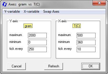
76 weight % [`Pb] in Cu(liq) Deleading of a Cu-1wt%Pb alloy: Graphical Output 1.0 Deleading of Cu-1wt.%Pb by Argon Vacuum Refining Example of «Open» Equilibrium Calculation: T=1200 C and P=0.001 atm weight Ar (grams) 9.2.6

77 Menu Window Parameters menu In the Parameters menu the user is given information on certain overall parameter values, e.g. the dimensions of the major data arrays. The user may also modify certain parameters which relate to output lists or which permit the interference with the execution of the calculations. The following slide shows the Parameter screen as a whole. Further slides are used to give details on the use of the parameters

78 Menu Window Parameters menu Dimensions frame Target Limits frame Dilute extrapolation frame Output Mass Units frame Print Cut-off frame Predominant Species frame Stop/Kill Window frame Help Additional information and extended menus are available for many of the items. Point to a frame heading or input box and then click the mouse-right-button

79 Parameters menu: Dimensions Frame The following slide gives information on the Dimensions Frame. This part of the Parameters menu is strictly for information of the user. NO changes may be made. The dimensions table lists the current and maximum size of some commonly used variables. The maximum values are fixed during compilation and can not be modified without recompilation. Increasing a maximum value would increase the size of the program and reduce execution speed. Except for «Species selected for products», «Components», and «Total selected solutions», please contact us if you consider that a particular dimension is too small. 10.1

80 Parameters menu: Target Limits Frame and Stop/Kill Button The following slides shows how Target limits may be changed and how the Stop/Kill button is activated/deactivated. Target Limits These values are the lower and upper limits of temperature, pressure, volume and alpha when these values are being calculated by Equilib. It is recommended that the default settings be used. Click on the «Target» frame in the Menu Window for details on how to specify a target. Stop and Kill Button When «checked» you are able to follow the progress of the equilibrium calculation and have the option to «stop» or «kill» the calculation should the program get hung up. This feature is only really useful for large and lengthy calculations, or those cases where the program is unable to converge. 10.2

81 Parameters menu: Predominant Species Frame The following slide shows how the Predominant Species frame is made use of. This input controls the execution of equilibrium calculations in which the number of species to be used exceeds the maximum number of species that may be used simultaneously. Predominant Species These are the number of predominant gaseous species (50 to 300) and pure solid and liquid species (50 to 300) that will be calculated when the Equilibrium option «Predominant» is selected. To improve the chances of convergence it is recommended that you use «300» in both cases. If you must reduce the number (for example because you have selected more than 100 solution species) then you should retain «300 gas» species and reduce only the number of solid and liquid species. The «log file» records the progress of the predominant calculation. If you get the message «- unable to calculate the standard state element(s)» it may be useful to consult this file. The log file will appear in the Results Window only if the «log file» box is checked. 10.3

82 Parameters menu: Dilute Extrapolation-Print Cut-off-Output Mass Units Frames This slide shows how use is made of the Dilute Extrapolation, the Print Cut-off and the Output Mass units frames. This value is used for extrapolating solute data outside its normal dilute concentration range stored in its solution database. The parameter is an advanced feature of the program and should not be modified from its default value (1.0e+6). In the Results Window, equilibrium products below this value are not printed. This is useful in large calculations where you want to limit unwanted output for insignificant species. The value must be in the range 1.0e-70 to 0.01 The value has no effect upon the results of the calculation. Normally the input reactants and output results are both in moles and mole fractions, or grams and weight per cent. This option enables you to have input moles and output weight, or vice versa. The equilibrium results are still the same, just the method of presenting the results is changed. Note, the same effect can be obtained using the "gram" and "mole" formats in the List Window. 10.4

83 Reactants screen options The following sixteen slides show how use is made of various options that can be found in the Reactants screen of the Equilib module. The use of arbitrary species formulae is shown in the following slide. Note that this option is very useful when only the input amount of the «arbitrary» species is important for the calculation. As soon as extensive property changes are to be calculated this kind of input is not permitted since the «arbitrary» species has a chemical formula but no thermodynamic properties. Thus the input cannot be used to calculate the state properties of the reactants. 11.0

84 Combining reactants into one composite chemical species There are 6 reactants The units are T ( C) and Mass (mol) You can combine the 3 matte components, 42 Cu + 25 Fe + 33 S, into one composite species, Cu 42 Fe 25 S 33. Likewise 0.79 N O 2 can become N 1.58 O <A> is a variable corresponding to the number of moles of air, <B> is a constant amount of SiO 2 defined in the Menu Window. Note: N1.58O0.42 Make sure you do not mix up the letter «O» and the integer «0». 11.1

85 Converting reactant mass units (mol g or lb) The input of mass units in the Reactants screen is not fixed to the use of the unit that was chosen as default. It is possible to «mix» mass units, i.e. to use the default for some and specific chosen units for others of the input substances. The following two slides show how this is achieved

86 Converting reactant mass units (mol, g or lb) Point the arrow in the mass input box to view the mass conversion. Point the arrow in the species input box to view the molecular weight. Note that no data are available for the composite chemical species. For example you may wish to specify the matte component in grams. 1. Right-click on the matte mass input box to open the mass menu. 2. Select: Convert this reactant amount to > g

87 Mixing reactant mass units of mol g and lb You can mix the mass units by including a 'mol', 'g' or 'lb' in the reactant amount. If the default mass units is mol, the following is equivalent to the above system: Or if you like, you can always explicitly specify the mass units for each reactant amount to make your reactants data entry independent of the default mass units. Note: When creating a composite species (for example Cu 42 Fe 25 S 33 and N 1.58 O 0.42 ) option «initial conditions» (Delta H, etc.) is disabled since there are no data for the species. the species is limited to 7 elements. For more than 7 elements use a mixture - refer to the Mixture module. 11.3

88 Importing a stream or mixture In addition to entering input substances by name/formula in the Reactants screen it is also possible to enter «groups» of substances as a whole package. Such groups can be either Mixtures or Streams. For the generation of Mixtures see the Slide Show on the Mixture Module. For the generation of Stream see below (slides and ). The following five slides ( to ) show the details of making use of Streams and Mixture in the Equilib input

89 Exporting and importing an equilibrated molten salt stream - CaCl 2 -NaCl-KCl-MgCl 2 This example: creates and saves an equilibrated stream - CaCl 2 -NaCl-KCl-MgCl 2 at 750 C. imports the stream into a new reaction performs various isothermal and adiabatic heat balances using the imported stream The units are T ( C), P (atm) and Mass (g). There are 4 reactants, total mass = 95g Possible product: FACT-Salt The final conditions are: T= 750 C P= 1 atm

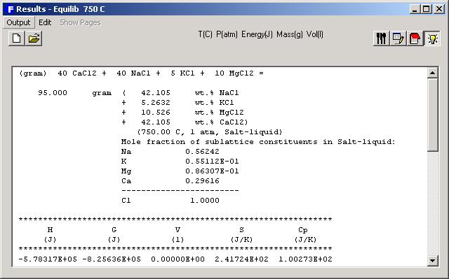
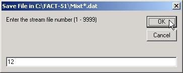
90 Saving an equilibrated stream Equilibrated molten salt

91 Importing the stream into a reaction Click on the [Mg-electrolyte] dropdown box to list the stream contents Initial Conditions check box is selected You can change the amount of [Mg-electrolyte] from its default value (95 g) Import the Mg-electrolyte stream by selecting it in the Edit Menu There are now 2 reactants: <A> MgCl 2 (s,25 C) + 95 [Mg-electrolyte] (stream,750 C) i.e. <A + 95> grams total. Note: You cannot change the initial T (750 C) or P (1 atm) of the [Mg-electrolyte] stream - these values, together with selected stream thermodynamic properties (H, S, G, C p, V), are stored in the stream file (mixt12.dat) and are imported into the calculation when Initial Conditions (DH, etc.) is checked

92 Equilibrated <0> and <5> MgCl g [Mg-electrolyte] stream at 750 C In the Menu Window FACT-Salt is the only possible product. Set <A> = '0 5' (i.e. alpha = 0 and 5), T = 750 C and P = 1 atm. The Results are: Calculated DH=4415 J this is the total energy required to heat 5 g MgCl 2 from 25 to 750 C and dissolve it into the molten salt. A = 0 Calculated DH=0 imported and equilibrated streams are the same. A =

93 Adiabatic <5> MgCl 2 (solid, 25 C) + 95 g [Mg-electrolyte] stream The output shows a calculated adiabatic temperature of C. Return to the Menu Window, set <A> = 5 and T(C) undefined ('blank') then specify an adiabatic reaction: DH =

94 Adiabatic <A> MgCl 2 (solid, 25 C)+ 95 g [Mg-electrolyte] stream at 725 C From the previous Results we know that the value of <A> should be 2-3 g. But Equilib requires that the calculated <A> be no more than 1.0. Return to the Menu Window, set <A> undefined ('blank'), set T(C) = 725 C, and specify an adiabatic reaction: DH = 0. The output shows:

95 Adiabatic <100A> MgCl 2 (solid, 25 C)+ 95 g [Mg-electrolyte] stream at 725 C This is resolved by entering <100A> MgCl 2 in the Reactants Window. Do not forget to check the Initial Conditions box. The calculation now gives <A> = , i.e. 100 x = g MgCl 2 (solid,25 C) are required to reduce the bath temperature to 725 C

96 Using Reaction Table input In addition to the two «group input» methods outlined above it is also possible to employ Reaction Tables from which the input amounts are read. Such Reaction Tables provide the opportunity to enter input amounts for cases in which non-linear changes of the amounts are needed. In the table each line contains for a given set of input substances the irregularly changing amounts. In the calculations the line number (Page number) will be treated as the independent parameter in order to sort the result tables. The Page number can also be used as an axis variable in the Result module

97 Reaction Table In the Reactants Window you specify a set of reactant amounts, for example: 1 mol CH mol C 2 H mol O 2 : With the Reaction Table you can specify many different sets of reactant amounts as well as their product temperatures and pressures - each resulting in a separate equilibrium calculation. To open the Reaction Table: click on the Reaction Table button or select Table > Reaction Table from the Menu Bar

98 Editing the Reaction Table Each set (row in the Reaction Table) generates a page in the Results Window. There is no limit to the number of sets. The Reaction Table may be created and edited here, or imported via a simple text or Excel spreadsheet. After creating the table, Close it and press Next >>

99 Reaction Table Results Window After the Reaction Table has been created click on the Table check box in the Menu Window to activate it in the calculation

100 Data search options The following three slides show how the various options in the Data Search menu are employed to select/deselect specific data entries in a database. It is shown how the Gas Ions, Aqueous Species, Limited Data and CxHy options are made use of. 12.0

101 Data Search Menu: gas ions, aqueous species, limited data Include gaseous ions (plasmas): Gaseous ion concentrations are only significant at high temperatures and only meaningful in plasma calculations. Gaseous ions add a component (the electron) to the calculation and increase the total number of gaseous species. This increases slightly the calculation time. For most practical calculations gaseous ions have no effect and so it is safe not to include them in the data search. Debye Shielding is automatically taken into account for plasmas in FactSage versions 5.5 and higher. Include aqueous species: Including aqueous species is only meaningful in aqueous (hydrometallurgical) calculations at or near room temperature. If your calculations are above 300 C there is no point in including the aqueous species. This option has no effect upon gaseous ions (plasmas). Include limited data compound (25 C/298K data only): Some solid and liquid compound species only have limited data - typically the Gibbs energy of formation at K but without Cp and enthalpy data. In Equilib these compounds are flagged as '25 C or 298 K only' in the List Window. Such species are automatically dropped from the calculation if the final temperature is above 25 C. In such a case the "activity" column in the List Window is blank. Since most of these species are unimportant and in most cases ignored anyway then there is little need to select this option. 12.1

102 Reactants window Data Search Menu: C x H y, databases Limit organic species C x H y : The main compound substances database contains several hundred organic species C x H y where the stoichiometric factor "x" can be large. These large organic molecules have little use in most inorganic calculations and are unlikely products in most equilibrium calculations. To drop large organic species from the data search you set "x" to the desired upper limit. For most calculations it is recommended you set x = 2, which means that organic molecules with 3 or more carbon atoms will be dropped from the data search. Databases: Opens the databases window. Databases may be added to or removed from the data search. For example private data entered through the Compound and Solution programs, or other commercial databases such as Thermo-Tech. If you have both FACT and SGTE databases then you use this option to tell the program to search both databases or search only one. Note: Clicking on the databases bar also opens the Databases window. Refresh: In the Data Search menu when you change a search option (gaseous ions, aqueous species, limited data) or database selection then Equilib will automatically 'refresh' the system with the new options and data. However, if changes to the databases are made via another program (for example Compound and Solution) you must click on Refresh" to update the current system. 12.2

103 Databases Window More information about coupled databases More information about the selected database. If 'coupled' is checked (this is the recommended setting) then compound and solution databases with the same nickname (for example FACT or SGSL) are treated as a group. For example, if you click on the '+' column in order to include the FACT compound database in the data search then the program automatically includes the FACT solution database. Likewise if you remove the SGSL solution database from the data search the program automatically excludes the SGSL intermetallic compound database. If 'coupled' is NOT checked then the databases can be included or excluded independently. However this is not recommeded since it can lead to misleading results. 12.3

104 Equilib Cooling Calculations The Equilib module enables you to perform cooling calculations and display the phase transitions and compositions during Equilibrium cooling Scheil-Gulliver cooling Full annealing of cast alloys Cooling Calculations - Table of Contents Section 13.1 Section 13.2 Section 13.3 Section 13.4 Section 13.5 Section 13.6 Table of Contents Phase transitions : FeO-MnO Simple equilibrium cooling : FeO-MnO Simple Scheil-Gulliver cooling : FeO-MnO Equilibrium cooling, plots: Al-Mg-Zn Scheil-Gulliver cooling, annealing casted alloy : Al-Mg-Zn-Mn 13.1

105 Temperature ( C) FeO-MnO : Phase transitions - binary phase diagram 1900 FeO-MnO binary phase diagram FeO - calculated MnO by Phase Diagram FactSage 1800 Slag <A> = X MnO = T liquidus = C Slag + Monoxide 1500 T solidus = C 1400 T FeO(melting point) = C Monoxide mole fraction MnO

106 FeO-MnO : Equilibrium phase transitions at X FeO = Binary system <1-A> MnO + <A> FeO. 2 Possible products: solid solution (MONO) liquid Slag (SLAG) 3 <A> = 0.5 T ( C) = 1500 and 1700 Equilib will calculate the equilibrium at X FeO = 0.5 for temperatures varying from 1500 C to 1700 C and will search for All phase transitions

107 FeO-MnO : Phase transitions showing liquidus and solidus Equilibrium liquidus Equilibrium solidus

108 FeO-MnO : Simple equilibium cooling L-Option 1 Right-click on the + column to open the SLAG extended menu and select L cooling calculation.to open the Cooling Calculation Window 2 Cooling Calculation Window select equilibrium cooling check transitions + summary click OK to close

109 FeO-MnO : Simple equilibium cooling step, T-auto and stop Equilibrium Cooling of SLAG cooling step 5 ( ) T-auto automatically calculates the starting T final mass 0 (i.e. stops after complete solidification) In equilibrium cooling the cooling step ( 5 ) defines the pages displayed in the Results Window. (i.e. every 5 degrees). The cooling step has no effect on the transitions or when 100% solidification is attained. Enter default starting temperature 1650 applied when T-auto is not used

110 FeO-MnO : Equilibrium cooling Summary and Transitions Summary Transitions

111 FeO-MnO : Equilibrium cooling - Liquidus and Solidus Liquidus Solidus

112 Scheil target phase The program performs a Gulliver-Scheil cooling calculation. That is, as phases precipitate from the Scheil target phase they are dropped from the total mass balance. Generally a value of T (the initial temperature) and a cooling step must be specified in the Final Conditions frame. Normally, the Scheil calculation is repeated until the Scheil Target phase disappears. However it is possible to stop the calculation by either specifying a second temperature in the Final Conditions frame, or by specifying a target mass. The Scheil target phase must be the gas phase or a real solution. If it is a liquid phase (such as FToxid-SLAG and Ftsalt-liquid) then the precipitates are generally solids - it would be unusual in this case to select and include other liquids or the gas phase in the calculation. If the Scheil target phase is the gas phase then the precipitates could be any or all of the other compound and solution phases. To activate a Scheil target gas phase, first select the gas species in the usual way. Then with the mouse-right-button click on the gas '+' check box in the compound species frame of the Menu Window - this will open the Species Selection window. Point to the '+' column of any selected gas species and then click with the mouse-right-button and then select «Scheil cooling gas phase». 13.3

113 FeO-MnO : Scheil-Gulliver cooling L-Option 1 Right-click on the + column to open the FACT-SLAG extended menu and select L cooling calculation.to open the Cooling Calculation Window 2 Cooling Calculation Window select Scheil-Gulliver cooling check transitions + summary. click OK to close

114 FeO-MnO : Scheil-Gulliver cooling step, T-auto and stop Scheil-Gulliver Cooling of SLAG cooling step 5 ( ) T-auto automatically calculates the starting T final mass 0 (i.e. stops after complete solidification) In Scheil-Gulliver cooling the cooling step ( 5 ) defines the calculation step (i.e. every 5 degrees). After each calculation any phase that precipitates from the solution phase is dropped from the total mass balance. The size of the step effects the calculated results. The smaller the step, the more precise the calculation and the longer the calculation time. Enter default starting temperature 1650 this is applied when T-auto is not used

115 FeO-MnO : Scheil cooling Summary and Transitions Summary Transitions

116 FeO-MnO : Scheil cooling Start and Stop Start of solidification at o C The size of the cooling step effects the calculated results. Here the step 5 o C gives o C. The end of Scheil solidification should be at o C the melting point of FeO. With a much smaller step, 0.1 o C, one obtains ~ o C.. End of solidification at o C

117 FeO-MnO : Scheil cooling incremental vs. accumulated Incremental Scheil solidification at 1500 o C Accumulated Scheil solidification at 1500 o C

118 Al-Mg-Zn : Equilibrium cooling X Mg =0.8 X Al =0.15 X Zn =0.05 Al-Mg-Zn polythermal liquidus projection calculated by Phase Diagram with data taken Al - Mg - Zn from FTlite Data FACT from FTlite light - FACT alloy light alloy databases Zn 1: 2: 3: 4: 5: 6: 7: 8: 9: 10: 11: 12: 1: 2: 3: 4: 5: 6: 7: 8: 9: 10: 11: 12: Four-Phase Intersection Points with Liquid AlMgZn_Tau / FCC_A1#1 / Laves_C14#1 AlMgZn_Tau / Beta_AlMg / Gamma AlMgZn_Tau / Beta_AlMg / FCC_A1#1 AlMgZn_Tau / Laves_C14#1 / Mg2Zn3 AlMgZn_Tau / Gamma / Phi Gamma / HCP_A3#1 / Phi FCC_A1#1 / Laves_C14#1 / Mg2Zn11 AlMgZn_Tau / Mg2Zn3 / MgZn FCC_A1#1 / HCP_Zn / Mg2Zn11 HCP_A3#1 / Mg51Zn20_<mg7zn3>_oi1 / MgZn AlMgZn_Tau / HCP_A3#1 / Phi AlMgZn_Tau / HCP_A3#1 / MgZn A = Zn, B = Mg, C = Al X(A) X(B) X(C) o C Mg MgZn HCP_A Phi 6 Mg2Zn Laves_C14 AlMgZn_Tau Gamma 0.6 HCP_Zn mole fraction Beta_AlMg T(min) = o C, T(max) = o C Mg2Zn11 FCC_A Crystallization path for Equilibrium cooling Alloy composition: 80 mol % Mg 15 mol % Al 5 mol % Zn Al 13.4

119 Al-Mg-Zn : Equilibium cooling L-Option Equilibrium Cooling of Liquid Al-Mg-Zn cooling step 10 T-auto final mass

120 Al-Mg-Zn : Equilibium cooling Summary of Results Liquidus temperature = C Constituent 1 is primary hcp formed between C and C Constituent 2 is a binary eutectic formed between C and C Microstructural constituents, and the phases in them

121 Al-Mg-Zn : Equilibium cooling Plot Results

122 Al-Mg-Zn : Equilibium cooling Plot Results Selection of species to be plotted - select all solids and elements for which Gram (max) >

123 Al-Mg-Zn : Equilibium cooling Plot Results Liquidus temperature = C Constituent 1 is primary hcp formed between C and C Constituent 2 is a binary eutectic formed between C and C

124 Al-Mg-Zn : Scheil cooling X Mg =0.8 X Al =0.15 X Zn =0.05 Al-Mg-Zn polythermal liquidus projection Al - Mg - Zn calculated by Data Phase from FTlite Diagram - FACT light alloy with databases data taken from FTlite FACT light alloy databases Zn 1: 2: 3: 4: 5: 6: 7: 8: 9: 10: 11: 12: 1: 2: 3: 4: 5: 6: 7: 8: 9: 10: 11: 12: Four-Phase Intersection Points with Liquid AlMgZn_Tau / FCC_A1#1 / Laves_C14#1 AlMgZn_Tau / Beta_AlMg / Gamma AlMgZn_Tau / Beta_AlMg / FCC_A1#1 AlMgZn_Tau / Laves_C14#1 / Mg2Zn3 AlMgZn_Tau / Gamma / Phi Gamma / HCP_A3#1 / Phi FCC_A1#1 / Laves_C14#1 / Mg2Zn11 AlMgZn_Tau / Mg2Zn3 / MgZn FCC_A1#1 / HCP_Zn / Mg2Zn11 HCP_A3#1 / Mg51Zn20_<mg7zn3>_oi1 / MgZn AlMgZn_Tau / HCP_A3#1 / Phi AlMgZn_Tau / HCP_A3#1 / MgZn A = Zn, B = Mg, C = Al X(A) X(B) X(C) o C Mg MgZn HCP_A3 > Mg2Zn3 Phi Laves_C14 AlMgZn_Tau Gamma 0.6 HCP_Zn mole fraction Beta_AlMg T(min) = o C, T(max) = o C Mg2Zn11 FCC_A Crystallization path for Scheil cooling Alloy composition: 80 mol % Mg 15 mol % Al 5 mol % Zn Al 13.5

125 Al-Mg-Zn : Scheil-Gulliver cooling L-Option Scheil Cooling of Liquid Al-Mg-Zn cooling step 10 check T-auto enter final mass

126 Graphical output of Scheil target calculation Calculation ends at temperature of final disappearance of liquid. Graph shows phase distribution

127 Al-Mg-Zn-Mn : Scheil cooling AZ wt.% Mn alloy Scheil Cooling of Liquid Al-Mg-Zn-Mn cooling step 10 check T-auto enter final mass

128 Al-Mg-Zn-Mn : Scheil cooling Summary and Transitions AZ wt.% Mn alloy: Summary 89.75Al-9Mg-Zn-0.25Mg (wt%) Transitions

129 Al-Mg-Zn-Mn : Scheil cooling - Microstructure Constituents Summary & Transitions Microstructure constituents of AZ wt.% Mn alloy after Scheil cooling. Final disappearance of liquid at C

130 Al-Mg-Zn-Mn : Scheil cooling and fully annealing cast alloy Scheil cooling and post equilibration (annealing) of Scheil microstructure: AZ91 alloy wt.% Mn CONS. PHASE TOTAL AMT/gram 1 1 Al8Mn E-04 Tracking microstructure constituents Output : Solidification temperature of C 2 1 HCP E Al8Mn E HCP E Al11Mn E HCP E Al4Mn E HCP E Al12Mg E Al4Mn E HCP E Phi E Al4Mn E Al11Mn E HCP E Tau E Al11Mn E HCP E MgZn E Tau E Al11Mn E-06 Amount & Average Composition of the HCP phase wt. % Mg Al Zn Mn ppm ppm ppm ppm ppm ppm ppm

131 Al-Mg-Zn-Mn : selecting HCP phase for full annealing 1 Point mouse to constituent 2 HCP_A3 and double-click 2 Click OK to recycle HCP_A

132 Al-Mg-Zn-Mn : HCP phase imported into Reactant Window Change mass from 100% => 100 g List of components in HCP phase

133 Al-Mg-Zn-Mn : Equilibrium calculation full annealing of HCP Anneal at 150 to 500 o C

134 Al-Mg-Zn-Mn : Plotting fully annealed HCP phase

135 Al-Mg-Zn-Mn : Graph of fully annealed HCP phase Equilibrium phase distribution in HCP phase of constituent 2 after annealing (HCP + precipitates)

136 Al-Mg-Zn-Mn : Graph of fully annealed HCP phase Equilibrium phase distribution in HCP phase of constituent 2 after annealing (HCP + precipitates)

137 Al-Mg-Zn-Mn : Tracking microstructure constituents log 10 (wt.%) log 10 (wt.%) Scheil cooling and post equilibration (annealing) of Scheil microstructure: AZ91 alloy wt.% Mn Tracking microstructure constituents 'Al 12 Mg 17 ' HCP Annealing of HCP in 2 Annealing: Phases vs T for HCP in the different microstructural constituents 'Al 99 Mn 23 ' Al 4 Mn Al 11 Mn 4 'Al 8 Mn 5 ' Amount & Average Composition of the HCP phase at o C wt. % Mg Al Zn Mn ppm ppm ppm ppm ppm ppm ppm 'Al 99 Mn 23 ' Temperature ( o C) Al 4 Mn 'Al 12 Mg 17 ' HCP Annealing of HCP in 3 Temperature ( o C) Al 11 Mn

138 Paraequilibrium and minimum Gibbs energy calculations - In certain solid systems, some elements diffuse much faster than others. Hence, if an initially homogeneous single-phase system at high temperature is quenched rapidly and then held at a lower temperature, a temporary paraequilibrium state may result in which the rapidly diffusing elements have reached equilibrium, but the more slowly diffusing elements have remained essentially immobile. - The best known, and most industrially important, example occurs when homogeneous austenite is quenched and annealed. Interstitial elements such as C and N are much more mobile than the metallic elements. - At paraequilibrium, the ratios of the slowly diffusing elements in all phases are the same and are equal to their ratios in the initial single-phase alloy. The algorithm used to calculate paraequilibrium in FactSage is based upon this fact. That is, the algorithm minimizes the Gibbs energy of the system under this constraint. - If a paraequilibrium calculation is performed specifying that no elements diffuse quickly, then the ratios of all elements are the same as in the initial homogeneous state. In other words, such a calculation will simply yield the single homogeneous phase with the minimum Gibbs energy at the temperature of the calculation. Such a calculation may be of practical interest in physical vapour deposition where deposition from the vapour phase is so rapid that phase separation cannot occur, resulting in a single-phase solid deposit. - Paraequilibrium phase diagrams and minimum Gibbs energy diagrams may be calculated with the Phase Diagram Module. See the Phase Diagram slide show. 14.1

139 Paraequilibrium and minimum Gibbs energy calculations Fe-Cr-C-N system at 900K Equimolar Fe-Cr with C/(Fe + Cr) = 2 mol% and N/(Fe + Cr) = 2 mol% For comparison purposes, our first calculation is a normal (full) equilibrium calculation Select all solids and solutions from FSstel database T = 900K 14.2

140 Paraequilibrium and minimum Gibbs energy calculations Output for a normal (full) equilibrium calculation 0.5 Fe Cr C N = E-02 mol BCC_A2#1 ( gram, E-02 mol) (900 K, 1 atm, a=1.0000) ( E-07 Cr1C E-06 Fe1C E-07 Cr1N E-06 Fe1N Cr1Va Fe1Va3) E-02 mol SIGMA ( gram, E-02 mol) (900 K, 1 atm, a=1.0000) ( Fe8Cr4Cr Fe8Cr4Fe18) E-02 mol HCP_A3#1 ( gram, E-02 mol) (900 K, 1 atm, a=1.0000) ( E-02 Cr2C E-05 Fe2C Cr2N E-03 Fe2N E-02 Cr2Va E-05 Fe2Va) E-03 mol M23C6 ( gram, E-03 mol) (900 K, 1 atm, a=1.0000) ( Cr20Cr3C Fe20Cr3C E-02 Cr20Fe3C E-03 Fe20Fe3C6) 4 phases are formed at full equilibrium 14.3

141 Paraequilibrium and minimum Gibbs energy calculations Fe-Cr-C-N system at 900K when only C and N are permitted to diffuse 1 o Click here 2 o Click on «edit» 3 o Click here 5 o calculate 4 o Enter elements that can diffuse 14.4

142 Paraequilibrium and minimum Gibbs energy calculations 0.5 Fe Cr C N = mol FCC_A1#1 ( gram, mol) (900 K, 1 atm, a=1.0000) ( E-03 Cr1C E-03 Fe1C E-02 Cr1N E-02 Fe1N Cr1Va Fe1Va1) Output when only C and N are permitted to diffuse System component Mole fraction Mass fraction Fe Cr N E-02 C E E E-02 mol SIGMA ( gram, E-02 mol) (900 K, 1 atm, a=1.0000) ( Fe8Cr4Cr Fe8Cr4Fe18) System component Mole fraction Mass fraction Fe Cr E-03 mol M23C6 ( gram, E-03 mol) (900 K, 1 atm, a=1.0000) ( Cr20Cr3C Fe20Cr3C Cr20Fe3C Fe20Fe3C6) System component Mole fraction Mass fraction Fe Cr C E-02 Fe/Cr molar ratio = 1/1 in all phases 3 phases are formed at paraequilibrium when only C and N are permitted to diffuse 14.5

143 Paraequilibrium and minimum Gibbs energy calculations Input when only C is permitted to diffuse Input when only N is permitted to diffuse Input when no elements are permitted to diffuse (minimum Gibbs energy calculation) 14.6