PRE- AND POST-PROCESSING TOOLS FOR NEXT-GENERATION SEQUENCING DE NOVO ASSEMBLIES. Sari S. Khaleel

Transcription

1 PRE- AND POST-PROCESSING TOOLS FOR NEXT-GENERATION SEQUENCING DE NOVO ASSEMBLIES by Sari S. Khaleel A thesis submitted to the Faculty of the University of Delaware in partial fulfillment of the requirements for the degree of Master of Science in Bioinformatics and Computational Biology Spring Sari Khaleel All Rights Reserved

2 PRE- AND POST-PROCESSING TOOLS FOR NEXT-GENERATION SEQUENCING DE NOVO ASSEMBLIES by Sari S. Khaleel Approved: Cathy H. Wu, Ph.D. Professor in charge of thesis on behalf of the Advisory Committee Approved: Errol Lloyd, Ph.D. Chair of the Department of Computer and Information Sciences Approved: Babatunde A. Ogunnaike, Ph.D. Interim Dean of the College of Engineering Approved: Charles G. Riordan, Ph.D. Vice Provost for Graduate and Professional Education

3 ACKNOWLEDGMENTS I would like to thank my advisor, Dr. Cathy Wu; and my committee members Dr. Chuming Chen, Dr. Shawn Polson, and Dr. Eric Wommack for the guidance, encouragement, and patience that they have provided me with over the past two years. I would also like to thank my friends, Phil Perry and Michael Turchiano, and my colleagues, Dan Nasko and Xia Bi who have supported me and enriched my life. This dissertation was made possible by funding from the National Science Foundation grant # MCB (to K.E. Wommack and S.C. Cary), the Gordon and Betty Moore Foundation s Marine Microbiology Initiative to (K.E. Wommack and S.W. Polson); and the U.S Department of Energy grant # DE-FOA (to C.H. Wu). I would like to acknowledge Craig Cary of the University of Waikato, New Zealand for his cooperation with my metagenome analysis projects, and Miguel Pignatelli from the Wellcome Trust Genome Campus, EBI for his assistance with the development of my tools and expanding my knowledge of bioinformatics programming. This dissertation is dedicated to my parents, Safaa and Wiaam Khaleel for their love, support, and guidance throughout my life, and to my brother, Waseem Khaleel, for being my brother and best friend. iii

4 TABLE OF CONTENTS LIST OF TABLES... v LIST OF FIGURES...vii ABSTRACT... x Chapter 1 INTRODUCTION PRE-PROCESSING OF NEXT GENERATION SEQUENCING READS AND DE-NOVO GENOME ASSEMBLY Next-Generation Sequencing Technology Error Profiles of Illumina and 454 Platforms De novo Genome Assembly Using the De Bruijn Graph Approach Review of Current Tools for Pre-processing NGS Reads ngsshort Conclusions DETECTION AND REMOVAL OF EXOGENOUS SEQUENCE ARTIFACTS FROM NGS READS Removing Primer/Adaptor Contamination in Literature The kmerfreq Algorithm Testing kmerfreq on 454 Reads of a Real Viral Metagenome CHIMERIC CONTIGS IN METAGENOME ASSEMBLIES Introduction to Metagenomics and Metagenome De Novo Assembly The Chimeric Contig Simulation and Analysis Pipeline Generation of Simulated Metagenomes: createmetagenomes Analysis of Read-to-Contig Alignment Information: contiganalyzer Analysis Results for Simulated Bacterial Metagenome Assemblies Conclusion CONCLUSION REFERENCES iv

5 LIST OF TABLES Table 4.1 Table 4.2 Table 4.3 Simulated 454 dataset and their Newbler de novo assembly statistics. Contig statistics were derived from each assembly s 454AllContigs.fna, excluding contigs shorter than 400 bp (read length). C.L. = contig length Analysis pipeline results for the simulated test dataset assemblies. The information shown in this table was derived from contig reports generated by analyzechimericcontigs (see section 2.4). chi contigs = chimeric contigs, sig-chi contigs = significantly chimeric contigs, sig-chi contigs with LCA > spp = significantly chimeric contigs where the rank of the LCA reported by NCBI s Taxonomy Browser was higher than species (genus and above), whereas other sig-chimeric contigs were formed by different species strains of the same organism Taxonomy reports for simulated metagenome assemblies. This table shows a subset of the Taxonomy report file produced by our pipeline for Newbler assemblies of the X10, X10_error, and X5 datasets, showing the top 18 organisms contributing to sigchimeric contigs. Organisms from the same species/genus are highlighted using the same color. Note that the percentage of (Not-) significantly chimeric contigs equals the percentage of (Not-) significantly chimeric contigs with an LCA rank higher than species + percentage of (Not-) significantly chimeric contigs formed by strains of the same species v

6 Table 4.4 Possible functions of chimeric regions on contigs with an LCA rank above genus. Several sig-slices from the Sig-slice report generated by analyzechimericcontigs (see section 4.4) were aligned against the nr/nt database using BLASTN (with the Entrez query field set to bacteria ). The table shows the dataset, slice ID (parent contig ID and slice location on contig in 1/100 th s of contig length), the LCA (and its rank), and the expected function of this region. The expected function of these slices was deduced from the BLAST report by choosing the most common feature of the subject sequences. Note that contig01335 was almost entirely chimeric (some slices are not shown in this table) and aligned to the rrna-16s ribosomal RNA sequence in members of the family Pasteurellaceae vi

7 LIST OF FIGURES Figure 2.1 Differences between Overlap and De Bruijn Graph Construction. Based on the set of 10 8-bp reads (A), we can build an overlap graph (B) in which each read is a node, and overlaps >5 bp are indicated by directed edges. Transitive overlaps, which are implied by other longer overlaps, are shown as dotted edges. In a de Bruin graph (C), a node is created for every K-mer in all the reads; here the K-mer size is 3. Edges are drawn between every pair of successive K-mers in a read, where the K-mers overlap by k -1 bases. In both approaches, repeat sequences create a fork in the graph. Note here we have only considered the forward orientation of each sequence to simplify the figure. Adapted from [35] Figure 2.2 Construction and Resolution of the DBG graph of a DNA sequence. The sequence at the top represents the polymorphismfree genome sequence, which is then sampled using shotgun sequencing with 7-bp reads (step 1). Some of the reads have errors (red). In step 2, the K-mers in the reads (4-mers in this example) are collected into nodes and the coverage at each node is recorded. There are continuous linear stretches within the graph, and the sequencing errors create distinctive, low-coverage features through out the graph. In step 3, the graph is simplified to combine nodes that are associated with the continuous linear stretches into single, larger nodes of various k-mer sizes. In step 4, error correction removes the tips and bubbles that result from sequencing errors and creates a final graph structure that accurately and completely describes in the original genome sequence. From [11] vii

8 Figure 2.3 Assembly of ngsshort-trimmed datasets using Velvet. Each trimmed dataset is named after the sequence of ngsshort trimming algorithms used to create it from raw reads. For (a), Contiguity is measured as the N50 contig length (C.L.). For (b) and (c), Correctness is measured as the ratio of length of contigs (Hit Contig Length, HCL) aligning to the C. elegans reference genome and the complete proteome database using BLASTN and BLASTX, respectively. Contiguity and Correctness were measured for contigs with C.L. >= 200 bp. In (d) and (e), Velvet performance is measured as the maximum RAM usage and runtime of the DBG building and manipulation step (velvetg) of Velvet, respectively. 5adpt = 5adpt[mp =100, list=illumina primers and adapters, search_depth = full_read_length, action=ka], nsplit5 = nsplit[n 5], ncutoff1 = ncutoff[n=1] = remove reads with any N bases, tera = TERA[avg =2], lqr = LQR[lqs =3, p 70%], mott= Mott[ml = 0.6], 3end = 3end[x=7]. For 3end, x was set to 7 to compare it to TERA[avg=2], which removed about 7% of bases Figure 3.1 BLASTN matches in nr/nt for Left1 and Left, the merged sequences of high-frequency left 8-mers detected by kmerfreq. BLASTN was run using word length = 7, and all other parameters were set to their default values. Only hits with E-value < 5 are shown in this figure Figure 4.1 Flow diagram of a typical meta-genome project. Dashed arrows indicate steps that can be omitted. From [57] Figure 4.2 The chimeric contig simulation and analysis pipeline Figure 4.3 The contiganalyzer pipeline Figure 4.4 Cladogram for a significantly chimeric contig. This cladogram was generated by contiganalyzer (step 7) for the largest contig in the X5 assembly. The LCA for this tree is the Phylum Proteobacteria viii

9 Figure 4.5 Types of slices in a chimeric contig. This is a section of the sliced coverage plot generated by contiganalyzer (step 7) for a contig in the X5 assembly. The X-axis shows the sources of each bases (represented by characters: A= Xylella fastidiosa 9a5c, B = Xylella fastidiosa M12), and the Y-axis shows the coverage for every base. A non-chi (non-chimeric) slice has one source, while a not-sig (not significant) slice is chimeric but not significant for analysis because it did not satisfy the coverage and/or length cutoffs (10, 20, respectively). Base sources of the sig-chi slice are suffixed with an asterisk. The parent contig of these slices is labeled sigchimeric because it had at least one sig-chi slice. Not-sigchimeric contigs have non-chi and not-sig chi slices but no sig-chi slices Figure 4.6 Location of sig-chimeric slices on contig Figure 4.7 Mean base coverage of significantly chimeric contigs (sig-contig) and their significantly chimeric (sig-) and non-chimeric (non-chi) slices ix

10 ABSTRACT High-throughput Next-Generation Sequencing (NGS) technologies have revolutionized and accelerated genomic analyses. However, their shorter read length and higher error rates in comparison to classical Sanger sequencing have hindered downstream analyses such as de novo genome assembly. Therefore, there is an urgent need to develop tools for quality control and pre-processing of NGS short-read data and perform systematical assessments of their impact on downstream analyses Many de novo assembly projects that use NGS include a pre-processing step where low quality reads and sequence artifacts are cleaned from NGS reads using unpublished in-house scripts. Although some open-source and commercial trimming scripts or pre-processing tools are available, a simple and comprehensive open-source toolkit with major trimming algorithms is currently lacking. Furthermore, most of the aforementioned assembly projects assess assembly by contiguity alone without evaluating the correctness of the assembled contigs. The problem of misassembly is complicated further in metagenomic assemblies by contig chimerism, which is caused by the co-assembly of reads from two or more genomes at regions of sequence similarity. Recently developed metagenomic assemblers attempts to solve this problem during assembly, but they are trained on short, high-coverage Illumina reads and not the long, low-coverage reads of 454, the preferred platform for metagenome sequencing. Contig chimerism affects downstream metagenome analyses, such as binning and gene prediction. x

11 Presented are methods and tools for pre- and post-assembly processing of NGS data. ngsshort (next-generation-sequencing Short Reads Trimmer), a tool written in Perl to implement many of the commonly used algorithms in trimming literature as well as methods developed by our group, was developed for pre-processing of NGS reads. ngsshort was tested on Illumina paired-end (PE) reads of the Caenorhabditis elegans genome, and its trimming methods were compared by the improvement in assembly contiguity as well as accuracy with BLAST. A particular problem in trimming NGS reads is the identification of adaptor sequences in NGS reads that may not be detected by regular text-search algorithms. This problem can be managed by the identification and removal of high frequency K-mers in reads using kmerfreq, our adaptor sequence detection and trimming tool. kmerfreq was tested on 454 reads of a viral metagenome specimen and the resulting improvement in assembly contiguity and assembler performance was evaluated. Finally, an analysis pipeline for contig chimerism in metagenomic assemblies of simulated 454 reads is presented and tested on a simulated bacterial metagenome. Our hypothesis is that chimeric contigs can be identified in a metagenomic assembly by the presence of unique coverage and polymorphism attributes that distinguish them from non-chimeric contigs. To train this post-assembly approach, a chimeric contig simulation and analysis pipeline was developed to study contig chimerism in assemblies of simulated metagenomes. The pipeline was used to simulate a bacterial metagenome and analyze and compare chimeric and non-chimeric contigs in its assembly. The results of this analysis may provide insight into coverage and polymorphism patterns in chimeric contigs, and may be useful for the detection of chimeric contigs in a real metagenome assembly. xi

12 Chapter 1 INTRODUCTION The emergence of Next-Generation Sequencing (NGS) technologies as a costeffective, high throughput alternative to classical Sanger technology has greatly benefitted biological research. Popular commercially available NGS platforms include Illumina (Genome Analyzer I, II and HiSeq), Roche (454 GS FLX Pyrosequencer) and ABI (SOLiD). Currently, the two major NGS platforms are Illumina and 454 [52, 60]. Unfortunately, all NGS platforms have major drawbacks in comparison to classical Sanger sequencing, including shorter read lengths, higher base-call error rates, and novel platform-specific artifacts. These sequencing errors result in poor quality assemblies that have shorter lengths and higher error rates when aligned to reference sequences [7]. In addition, the high throughput and short length of NGS reads (especially Illumina and ABI-SOLiD) make classical Overlap-Layout- Consensus (OLC) assembly algorithms obsolete. Instead, short high-throughput NGS reads are usually assembled using the de Bruijn Graph (DBG) approach, in which reads are decomposed into K-mers that in turn become the nodes of the DBG [37, 45]. The DBG approach has several drawbacks that include sensitivity to sequencing errors, as miscalled bases produce erroneous K-mers that result in increasing the DBG complexity, which can lead to longer runtime, more memory overhead, and more importantly, poor assemblies [7]. Consequently, many assembly projects include a pre-processing step where NGS data is quality-trimmed using a combination of trimming methods. Although 1

13 some open-source and commercial trimming scripts or pre-processing tools are available, a simple and comprehensive open-source toolkit that includes all the major trimming and contaminant detection methods is currently lacking. Chapter 2 covers the problem of pre-processing NGS reads and their subsequent assembly using De Bruijn Graph assemblers. General problems of the Illumina and 454 platforms are reviewed first, followed by a discussion of the DBG assembly algorithm and its popular assemblers and a review of trimming algorithms used in literature as well as commonly used trimming packages/scripts for preprocessing NGS reads. Chapter 2 ends with presenting ngsshort, an NGS reads trimming tool that implements most of the commonly used sequence-trimming methods in NGS literature as well as methods created by our group. ngsshort methods are applied to Illumina GA II paired-end (PE) reads of the Caenorhabditis elegans genome, which are subsequently assembled using several popular DBG assemblers. Individual trimming methods of ngsshort are compared by measuring their resulting improvements on assembly contiguity and correctness with BLAST, and then the combination of trimming methods that produces the greatest improvement in both measures is determined. Chapter 3 covers the problem of detection and removal of sequence artifacts, a major step in NGS trimming. Most trimming tools search for a user-supplied list of known platform sequence artifacts in reads using direct text-search. These methods often do not allow for mismatches and cannot adapt to the possibility of primer/adaptor sequence fragmentation. The alternative approach proposed in this chapter for primer/adaptor trimming from NGS reads is done in two steps: The first step is the detection overrepresented K-mers in the 5 - and 3 -ends of reads sampled 2

14 from the dataset using an approximate hash table (a hash that uses approximate matching for key lookups), as these K-mers may represent adaptor/primer sequences; the second step is to trim out these over-represented sequences from the dataset reads. This approach is implemented in kmerfreq, a tool developed in Perl (with multiprocessing in order to manage high throughput data) as a pre-processing step for NGS reads. kmerfreq was tested on 454 reads of a viral metagenome specimen. To evaluate kmerfreq s detection function, its detected sequenced were aligned against NCBI s nr/nt database using BLASTN. To evaluate the impact of removing these sequences, the subsequent improvement in de novo assembly of these reads was measured for assemblies done using the OLC assemblers Phrap [15] and Newbler. The problem of misassembly is more complicated in metagenomic assemblies due to the lack of a reference sequence to use for evaluating assemblies [28]. This complicates downstream analyses, such as binning and gene prediction. In addition, metagenome assembly suffers from contig chimerism, reads from different taxonomic groups co-assembling into the same contig [28, 42, 50]. Recently developed metagenome-specific assemblers are based upon DBG assembly and are trained only on high-coverage short Illumina reads, and are not reliable for assembly of low-coverage reads from the 454 platform, the more popular platform for metagenome assembly. Therefore, Newbler, 454 s native OLC assembler, remains the main assembler for 454 reads although it was not designed for metagenome assembly. Chapter 4 discusses the problem of contig chimerism. Our hypothesis is that base coverage and polymorphism information can be used to differentiate chimeric from non-chimeric contigs. To test this hypothesis, a chimeric contig analysis pipeline 3

15 that generates simulated NGS reads of artificial metagenomes and analyzes the coverage and polymorphism patterns of non-chimeric and chimeric contigs assembled from these reads is presented. The goal of the pipeline to find a set of coverage and polymorphism features that can be used to identify potentially chimeric contigs in assemblies of real metagenomes with unknown source species. Chapter 4 concludes by presenting the findings from running our analysis pipeline on a simulated bacterial metagenome and discussing differences between chimeric and non-chimeric contigs and examine the chimeric regions of these contigs at which reads from different species co-assemble. Finally, the conclusions of this dissertation are summarized in chapter 5. 4

16 Chapter 2 PRE-PROCESSING OF NEXT GENERATION SEQUENCING READS AND DE-NOVO GENOME ASSEMBLY The disadvantages of NGS include higher error rates and shorter read lengths in comparison to classical Sanger sequencing. In addition, the high throughput of these short reads has led to using the De Bruijn Graph (DBG) approach for their assembly using recently developed and not well-optimized algorithms. The higher error rate of NGS data and the limitations of DBG assembly algorithms have led to emphasis on pre-processing NGS reads using some trimming methods that usually include the removal of reads with uncalled N bases and adaptor sequences as well as some form of quality filtering. However, most assembly projects perform this pre-processing step using unpublished in-house scripts, and currently popular and freely available trimming tools do not implement all popular trimming algorithms and lack essential features for managing NGS reads and their platform-specific errors. This chapter begins by discussing NGS platforms, specifically secondgeneration, cyclic array sequencing platforms, and focuses on the most common of these platforms, Illumina and 454, discussing their error profiles. Next, the De Bruijn Graph (DBG) assembly method and its drawbacks are presented. The chapter concludes by presenting ngsshort, a powerful tool written in Perl to manage Single or Paired-end NGS data in the popular FastQ file format as well as Illumina s native qseq format, with special trimming methods for Illumina reads. ngsshort allows users to trim and filter reads using varying combinations of popular trimming methods 5

17 in literature as well as methods developed by our group. ngsshort is tested on Illumina GA II datasets and the resulting improvements in assembly contiguity, correctness, and assembler performance are evaluated in order to determine the best combination of ngsshort methods and parameters for NGS read trimming. 2.1 Next-Generation Sequencing Technology Until recently, the overwhelming majority of DNA sequence production has relied on some version of the Sanger biochemistry [32, 52]. The need for a cheaper, faster and more flexible alternative to Sanger sequencing has driven the development of new, next-generation technologies [52]. The cheap cost, high throughput and high coverage offered by NGS make the technology available to researchers in many old and newly emerging fields of life sciences, such as genomics, transcriptome studies, metagenomics, etc. In addition to its lower cost, major advantages of NGS over Sanger sequencing include parallelization (over 100 reactions versus 96 or 384- channel capillary systems), and the removal of cloning, the main bottleneck of Sanger Sequencing. Cloning is not fully automated, is expensive, and since the target vector is bacterial chromosomes, cloning is sometimes biased against certain DNA sequences that are not easily clonable. In contrast, NGS uses PCR to generated amplicons from fixed DNA segments [52]. Shendure et al. [52] classified alternative strategies for DNA sequencing into several categories: (i) microelectrophoretic methods, (ii) sequencing by hybridization, (iii) real-time observation of single molecules, and (iv) cyclic-array sequencing. Cyclic-array sequencing is currently the most common of these technologies and most of the major, commercially available NGS platforms are implementations of cyclic array. Cyclic array is also known as second generation sequencing or sequencing- 6

18 by-synthesis, that is, serial extension of primed templates [32, 52]. The most common and commercialized implementations of NGS include 454 Genome Sequencers (Roche Applied Science; Basel), Illumina (Genome Analyzer I, II, and HiSeq). IIllumina; Sang Diego), the SOLiD platform (Applied Biosystems; Foster City, CA, USA), and the HeliScope Single Molecule Sequencer technology (Helicos; Cambridge, MA, USA) [52]. In this dissertation, the term NGS will be used to refer specifically to sequencing-by-synthesis platforms. 2.2 Error Profiles of Illumina and 454 Platforms Currently, the two major NGS platforms are Illumina and 454. Illumina offers high throughput, short (~100 bp with Illumina GA II, ~150 bp with HiSeq) reads at relatively low cost, making it the more popular platform for genome re-sequencing (sequencing a genome with a known reference sequence to detect small mutations, SNPs, etc), de novo genome and transcriptome assembly, seq-based studies (RNA-seq, ChIP-seq), and quantitative analysis based on the number of sequence segments [37, 52]. 454, on the other hand, offers lower throughput, long (~400 bp with GS FLX Titanium) reads, making it the popular platform for metagenomics and other fields where long read length is essential [52, 60]. Several studies have been done to analyze the error profiles of NGS platforms [18, 20, 37, 55], and their evaluations of the Illumina and 454 error profiles can be summarized under the following metrics: 1. Base-call quality and alignability of reads to reference: On average, 55% of Illumina GA reads passed quality filters, of which approximately 77% aligned to the reference sequence. In contrast, approximately 95% of 454 reads uniquely aligned to the target sequence [18]. 7

19 2. Coverage variation: An often-described property of Illumina and 454 profiles is coverage variation [18, 20, 37, 55], which has been attributed to the inherent bias of polymerase chain reaction (PCR) amplification during sample preparation [18], or formation of secondary structures in single-stranded DNA (ssdna) [56]. AT-rich repetitive sequences showed lower coverage [18], while GC-rich region had higher error rates [37]. Harismendy et al. [18], noticed an over-representation of amplicon end sequences: These regions, which represented only 2.3% of their targeted sequence, accounted for up to 56% of sequenced base pairs from Illumina GA technology in contrast to only 5% of 454 bases. This difference in platform performance was attributed to library preparation process. For 454, the emulsion PCR (epcr) reaction seems to have a tendency for generation of duplicate reads (multiple reads from a single template), which occur when amplified DNA attaches to empty beads during epcr, or when the optical signal during sequencing bleeds into the space of an adjacent empty well [14]. 3. Error rates: Illumina sequencers result in more substitution-type miscalls than indel-type miscalls, while 454 sequencers result in more indel-type miscalls than substitution-type miscalls [22]. The high frequency of indel miscalls are caused by the difficulty of correlating the intensity of light produced by the epcr when the polymerase runs through a homopolymer with the actual number of nucleotide positions. 8

20 2.3 De novo Genome Assembly Using the De Bruijn Graph Approach The long read length (~1000 bp) and low throughput of ABI-Sanger reads allowed them to be assembled using the classical Overlap-Layout-Consensus (OLC) approach. In the Overlap phase, overlap discovery involves all-against-all, pair-wise read comparison. Overlap candidates must share K-mers that are used as alignment seeds. Next, an approximate read layout is constructed from manipulation of the overlap graph. In the consensus phase, progressive pair-wise alignments are used compute an optimal multiple sequence alignment [11, 35]. Newbler, the native assembler of the 454 platform, implements the OLC algorithm [35]. Unlike ABI-Sanger and 454, NGS technologies like Illumina and ABI-SOLiD generate far shorter reads with far higher coverages (30 to even 100X coverages for Illumina and SOLiD in comparison to the 8X coverage typical of Sanger sequencing projects). Furthermore, the shorter read length of NGS reads requires many more reads to generate the same level of coverage as that of Sanger. This results in very large datasets of short read sequences that not only make the read-centric OLC method computationally unfeasible, but it also makes it seemingly impossible to find heuristics to resolve the large number of overlaps between short reads [11]. However, pioneering work by Pevzner and colleagues in the late 1980s and Idury and Waterman in the mid-1990s introduced a different framework for handling assemblies. This framework utilizes the de Bruijn Graph (DBG) data structure instead of the overlap graph [11, 35, 43]. The DBG consists of very small, fixed-length subsequences known as K-mers (K is usually 19 or higher), and was originally developed for combinatorial mathematics [11]. In the DBG approach, the reads are decomposed into K-mers that in turn become the nodes of a DBG. This allows compressing the massive read dataset by 9

21 converting it into a K-mer frequency table where, regardless of the number of a K- mer s occurrences in the read dataset, it is represented only once in the table. A directed edge between the DBG nodes indicates that the K-mers on those nodes occur consecutively in one or more reads. Given perfect data, i.e., error-free K-mers providing full coverage and spanning every repeat, the K-mer graph would be a de Bruijn graph and it would contain an Eulerian path that traverses each edge exactly once, which is equivalent to the genome sequence, making assembly a by-product of the graph construction [11, 35]. Figure 2.1 shows the basic approach for constructing Overlap and de Bruijn graphs from the same set of reads. 10

22 Figure 2.1 Differences between Overlap and De Bruijn Graph Construction. Based on the set of 10 8-bp reads (A), we can build an overlap graph (B) in which each read is a node, and overlaps >5 bp are indicated by directed edges. Transitive overlaps, which are implied by other longer overlaps, are shown as dotted edges. In a de Bruin graph (C), a node is created for every K-mer in all the reads; here the K-mer size is 3. Edges are drawn between every pair of successive K-mers in a read, where the K-mers overlap by k -1 bases. In both approaches, repeat sequences create a fork in the graph. Note here we have only considered the forward orientation of each sequence to simplify the figure. Adapted from [35]. Sequencing errors complicate K-mer graphs because a single miscall will result in creating a new K-mer sequence that adds an additional branch within the de Bruijn Graph. However, many errors are easily recognized by their structure in the graph. For example, errors at the end of a read usually create K-mers that occur only once, and therefore form dead-end tips in the graph. Errors in the middle of a read create alternate paths called bubbles that terminate at the same node (Figure 2.2). DBG assemblers search for these localized graph structures in an error correction phase and remove the error nodes and other low coverage nodes [11]. Mate-pair information can be used to resolve ambiguity, using the coverage at each node to identify repeats, and by searching for unique paths through the graph consistent with the mate pairs [11, 35 63]. Popular freely available DBG assemblers include Velvet [63], ALLPATHS [4], ABySS [54], and SOAPdenovo [31]. 11

23 12

24 Figure 2.2 Construction and Resolution of the DBG graph of a DNA sequence. The sequence at the top represents the polymorphism-free genome sequence, which is then sampled using shotgun sequencing with 7-bp reads (step 1). Some of the reads have errors (red). In step 2, the K-mers in the reads (4- mers in this example) are collected into nodes and the coverage at each node is recorded. There are continuous linear stretches within the graph, and the sequencing errors create distinctive, low-coverage features through out the graph. In step 3, the graph is simplified to combine nodes that are associated with the continuous linear stretches into single, larger nodes of various k-mer sizes. In step 4, error correction removes the tips and bubbles that result from sequencing errors and creates a final graph structure that accurately and completely describes in the original genome sequence. From [11]. By breaking reads into shorter K-mers and processing these K-mers instead of reads, the K-mer graph construction discards long-range continuity information in the reads that are longer than their constitutive K-mers [35]. Repeats longer than K lead to tangled K-mer graphs that complicate the assembly problem, and complete read information can be essential for resolving long repeat or ambiguous regions that cannot be resolved using the K-mer graph or mate pair information [11, 35]. Furthermore, unlike the overlap graph, the DBG is not read coherent, i.e., there may be paths (resulting from K-mer alignment) through the graph that form a sequence that is not supported by the underlying reads. For example, if the same K-mer occurs in the middle of two reads, but the reads do not otherwise overlap, the corresponding DBG for those reads contains a branching node instead of two separate paths [11]. Another potential drawback of the DBG approach is that graph construction can require an enormous amount of computer resources [35]. Unlike conventional overlap computations, which can be partitioned into multiple jobs with distinct batches of reads (overlaps can be discovered in parallel with a matrix partition), the construction 13

25 and analysis of a DBG is not easily parallelized [35]. As a result, DBG assemblers such as Velvet [63] and ALLPATHS [4], which have been used successfully on bacterial genomes, would require several terabytes of RAM for assembly of the human genome, which is far more memory than is available on most computers. Currently, ABySS [54], SOAP [31] and CLCBio [5] are the only DBG assemblers known to be capable of assembling a mammalian genome [35]. All three assemblers use some form of parallelization to divide the memory load, as well as early correction of the DBG to remove erroneous K-mers that would otherwise add more complexity to the graph, thus increasing memory usage [5, 11, 31, 35, 54]. Finally, current DBG assemblers do not include base-call quality in graph construction, and do not produce quality score information for assembled contig bases. For these reasons, many sequencing projects (especially metagenome projects where read length matters for better homology detection [60]) prefer the relatively longer 454 reads (~400 bp with Titanium FLX) over Illumina reads (100 bp with GA II, ~150 bp with HiSeq). Instead of DBG assembly, 454 reads are assembled using Newbler which implements OLC instead of DBG, uses read quality score and flow information in OLC construction, and produces quality scores for assembled contig bases, along with complete read-to-contig alignment information [35]. 2.4 Review of Current Tools for Pre-processing NGS Reads Due to the problems of NGS, assembly projects that use NGS data include a pre-processing step where NGS data is quality-trimmed. This section reviews the pre-processing steps used by several recent assembly projects [1, 8, 9, 22, 34, 40, 54, 61, 64] that used Illumina and 454 data, as well as popular NGS-trimming software [5, 7, 10, 21, 16, 26, 30, 56, 41, 49]. Trimming steps that were used by all assembly 14

26 projects and provided by most trimming software include removing reads with uncalled N bases, and the detection and removal of adaptor sequences using direct text-search algorithms to search for user-specified adaptor sequences (usually the platform s known PCR primers, linkers and adaptors) in the reads set. To our knowledge, only CLC s commercial genomics workbench allows for the modification of the text-search algorithms used for adaptor sequence detection. An additional step done by a few assembly projects [1, 17] is to trim a number of bases from the 3 -end of all reads because of low base-call quality at the 3 -ends of reads [7, 20, 37]. Multiple trimmed datasets are generated by trimming different arbitrary numbers of bases from the 3 -end of reads, and are assembled at different K- mer lengths with a DBG assembler like Velvet. The chosen dataset (and thus the number of 3 bases that was removed from all of its reads) is the one with highest contiguity assembly. This method is inefficient because it relies on selecting an arbitrary set of numbers, treats all reads as if they all have the same quality scores at their 3 -ends, and requires assembly of multiple datasets using different arbitrary K- mer lengths, which is computationally expensive. Finally, the correctness of these trimmed datasets is not evaluated by comparison to a reference sequence. A less crude approach involves a sliding window algorithm that tries to extract a substring of read bases whose first and last base quality scores exceed a specified cutoff. This dynamic trimming step [7, 16, 26] is still arbitrary when it comes to determining the quality score cutoff and sliding window length, and can result in highquality reads that are still skipped during DBG assembly because they were trimmed to lengths shorter than the K-value (K-mer length) used by the DBG assembler, which requires all reads to be at least longer than K bases [63]. 15

27 An additional complication of trimming is the special case of mate pairs. As we mentioned earlier, mate pairs are important for repeat resolution and scaffolding, especially for DBG assemblers where long reads are broken down into short K-mers that are usually shorter than repeat regions. Most NGS platforms, especially Illumina, produce PE or mate pair reads. Mate pairs are usually listed in two separate files: the forward direction reads are in a file suffixed with _1, and their reverse direction mate reads are in a file suffixed with _2 in the same order of reads in the _1 file. During PE assembly, assemblers take one read from each mate file and use them only if the header of the read from _1 matches the read from _2. Moreover, a pair will still be skipped if either or both of its reads are shorter than the K-mer length used by the DBG assembler. Given the importance of mate pairs and the important ordering and length conditions for using their information, it was surprising to find that most of the available trimming tools do not trim mate pair files as a unit. Instead, they trim each mate file separately, which can result in removing some reads from the _1 file, while their mates in the _2 file are not removed (and vice versa), thus ruining the mate pair ordering for the two files. To our knowledge, the only freely available platforms that manage mate pairs are Btrim [26] (in a secondary step following separate mate file trimming), and NGS QC [41]. Except for NGS QC, none of the available toolkits implement multiprocessing to manage large NGS read datasets, especially the short reads of the high coverage Illumina and ABI-SOLiD platforms. Despite the popularity of the Illumina platform, none of the software tools that we reviewed offer Illumina-platform specific trimming methods or manage the direct qseq-format output of Illumina, which included Failed_Chastity filter information 16

28 that is very useful for trimming and can greatly improve assembly [22] but is lost during conversion to FastQ or FastA + qual files prior to trimming. Another unique feature of Illumina qseq format that is usually lost during quality score conversion from Illumina s ASCII-to-Phred mapping to the standard Sanger mapping is Illumina s B quality score, which in Illumina jargon means unknown quality score. None of the platforms reviewed managed this case or try to trim B -scored bases, and only one assembly project [12] managed it using unpublished in-house scripts that process raw qseq files. Finally, we could not find a toolkit that included all popular trimming methods and was used by many assembly projects. Instead, most of the assembly projects that were reviewed [1, 8, 9, 22, 34, 40, 54, 61, 64] do not use these open-source toolkits and instead perform trimming using their own unpublished in-house scripts, with arbitrary parameters that are tailored to their NGS data. 2.5 ngsshort ngsshort (NGS Short Read Trimmer) is a tool written in Perl 5.6 to trim Single or Paired-end reads in the popular FastQ read format or Illumina s native qseq format using all of the popular trimming methods used in NGS assembly projects and tools, as well as methods developed by our group. ngsshort uses multiprocessing to manage high throughput data and reduce running time. Another unique feature of ngsshort is that it was designed to manage Paired-End (PE) reads using PE-specific modules. ngsshort can be easily incorporated as a pre-processing step for most NGS transcriptome and genome assembly pipelines to improve the contiguity and correctness of assembly as well as reducing the memory usage for the assembly process. 17

29 The following methods are implemented by ngsshort: (1) 5adpt[mp,list,approx_match_modifiers,search_depth,action], which detects (at a match percentage mp and up to a depth of search_depth) 5'-adaptor/primer sequences loaded from list (which is defaulted to Illumina library primers and adaptor sequences) and removes them from reads. 5adpt allows users to implement approximate matching using the Levenshtein edit distance implementation in CPAN s String::Approx module [19]. This module allows approximate matching using a simple percentage cutoff, or using detailed modifiers: the number of allowed insertions, substitutions, and deletions. This feature, accessible through the approx_match_modifiers option, allows 5adpt to be modified to adapt to specific platform features and error profiles. For example, one should expect more indels over substitutions for 454 reads, and expect the opposite for Illumina reads. After an adapter/primer/linker sequence (or fragment) is matched and trimmed out of the read, action allows users to specify what to do with the read: it can be removed completely (action=kill-read, kr) or trimmed to the base 5 to the detected artifact string (action=kill-after, ka). (2) nperc[p] and (3) ncutoff[n], which filter out reads with uncalled N bases whose percentage or number are >= p or n, respectively. ncutoff[n =1] can be used to replicate the commonly used pre-processing step of trimming out reads with any N bases. (4) nsplit[l], which detects strings of uncalled N bases whose length is >= l, removes them from the read, and then splits the read around the detected N -string into two 18

30 smaller daughter reads. This method was developed by our group to remove N- bases from reads without having to remove the entire read and lose its information. nperc, ncutoff and nsplit are important for removing N bases because they usually have low quality scores, and DBG assemblers discard reads with such bases [54], or simply convert them to an arbitrarily-chosen nucleotide like A [63]. (5) 3end[x] and (6) 5end[y], which trim x and y bases from the 3' and 5' ends of all reads. (7) TERA[avg], is a method that I developed as an alternative to 3end. Unlike 3end, TERA trims the 3'-end of each read differently depending on it base-call quality scores. Starting at the 3'-end, the running average quality score (RAQS) for each base is calculated until it exceeds a cutoff, avg, at a base X; all bases 3' to X are then discarded. A good read with high quality (above avg) bases at its 3'-end will not be trimmed by TERA, while a low quality read may be trimmed more than other reads. (8) Mott[ml], is a quality-window extraction algorithm (i.e., it can trim both the 5' and 3' ends of a read). Starting at the 3'-end of a read, it counts the running sum of (ml - P error ) values, RSMLP, for each base in the read (P error of a base = 10-Q/10), it extracts the string from the first base with RSMLP > 0 to the base with the highest RSMLP. Mott method was adapted from the CLC Bio Genomics Workbench [5]. Mott is also similar to the QRL algorithm used by [8]. (9) LQR[lqs, p], which reads with over p% of bases whose quality score is under lqs. It is similar to algorithms used in [5, 16, 22]. 19

31 (10) qseq0 and (11) qseqb[n,mode,action] are methods specifically designed for Illumina reads. qseq0 removes qseq reads that did not pass the Failed_Chastity filter, which was shown to greatly improve assembly contiguity and correctness (Illumina technote, 2010). qseqb trims out reads with more B -scored bases than n. Illumina s B score means unknown quality score and bases with such scores are usually trimmed out along with bases 3' to them [8, 12]. Unlike qseq0, qseqb can be used with Illumina reads in the FastQ format after switching their ASCIIto-Phred score mapping from Sanger back to Illumina using switch_scores (see below). At mode= local, qseqb[n] will remove reads with >= n B -scored bases. At mode= local, qseqb[n] will search for a string of consecutive B - scored bases no shorter than n. If such a string is detected, the read can be removed completely (action=kill-read, kr) or trimmed to the base 5 to the detected B - scored string (action=kill-after, ka). A limited implementation of qseqb with mode=local and action=ka is used by [12]. (12) switch_scoring is not a trimming feature, but it allows switching the ASCII-to- Phred mapping of base-call quality scores between Illumina and Sanger mapping, which restores original Illumina-scoring for FastQ-formatted Illumina reads downloaded from NCBI s short read archive, including the aforementioned B - scoring of bases that can then be trimmed using qseqb. DBG assemblers will skip a PE read pair in paired-end assembly mode if either of its reads is shorter than the K-mer length used for assembly. To avoid trimming reads to lengths smaller than the K-mer size used for assembly, ngsshort enforces a global minimum read length limit variable, min_rl, on TERA, 3end, 5end, and Mott 20

32 methods to stop trimming when a read s length = min_rl. So, if the highest K-mer length used for assembly was 41, we set min_rl to 42 bp. Another special case of PE read trimming is widowed mates: if a read pair had one trimmed-out read and another intact read, ngsshort saves this widowed read in a separate single reads file that is co-assembled with the PE reads file. This approach was suggested by Daniel Zerbino (personal communication, 2011) and is used by [8] and [41]. ngsshort was designed in object-oriented Perl where the main object is a READ object. Every time ngsshort parses the next (qseq, FastQ, FastA) read from its input reads file, a READ object is created for every read to hold its attributes (most importantly, the header, the sequence, and the quality score strings of the source read, and the Failed_Chastity filter of qseq-format reads). Trimming methods act on the READ object s components and are independent of the reads file s original format, which makes it easy to implement additional trimming methods or have different output formats in ngsshort since the design is format-independent. ngsshort was tested on a publically available (from NCBI Short Read Archive, Accession Number: SRX026594) C. elegans genome, sequenced with Illumina Genome Analyzer II, consisting of 3.3 million PE 100-bp reads (insert size: 356) which totaled to about 6.8 billion base pairs. This dataset was chosen because it was relatively complex (multicellullar eukaryote with ~100 Mbp genome, consisting of 7 large chromosomes), had an annotated reference genome and transcriptome, and used a manageable memory overhead when assembled with Velvet (maximum RAM usage was ~70 GB at K = 23, minimum was ~20 GB with K=41 on most of our machines). 21

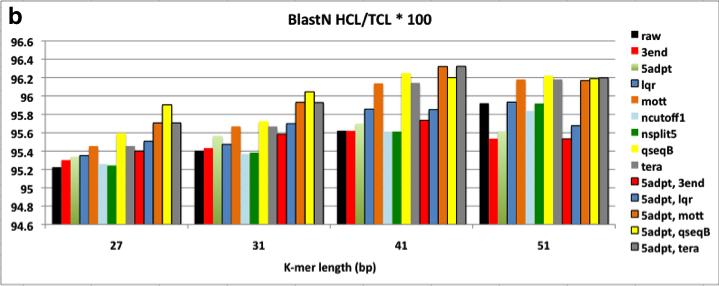
33 A trimmed reads dataset was produced for each method by running ngsshort to implement this method on the raw C. elegans genome dataset. The min_rl was set to 52 bp, which was greater than all K-mer lengths used for assembly. Assembly was done using the popular DBG assembler Velvet (version ) at different K-mer lengths (27, 31, 41, and 51 bp). ngsshort and Velvet were run on X86_64 Fedora Core 14 server with 256G RAM and 64 CPU/Core (2GHz). ngsshort was run using 60 threads, and the average runtime was 20 minutes per trimming job with a maximum RAM usage of ~200 MB for the total of the 60 threads. Assembly correctness was evaluated by aligning contigs against the C. elegans reference genome and complete proteome database using BLASTN and BLASTX (coverage i.d. = 90, e-value = ), respectively. Figure 2.3 shows N50 Contig Length (C.L.), BLAST correctness, and assembler performance results for these assemblies. 22

34 23

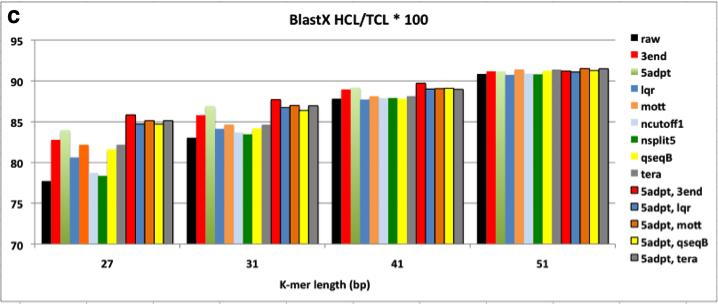
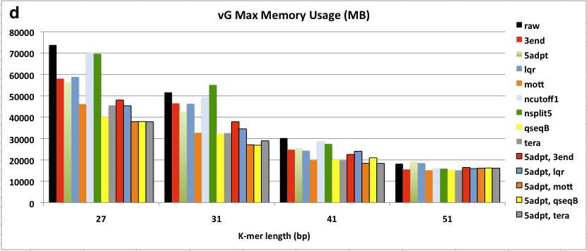
35 Figure 2.3 Assembly of ngsshort-trimmed datasets using Velvet. Each trimmed dataset is named after the sequence of ngsshort trimming algorithms used to create it from raw reads. For (a), Contiguity is measured as the N50 contig length (C.L.). For (b) and (c), Correctness is measured as the ratio of length of contigs (Hit Contig Length, HCL) aligning to the C. elegans reference genome and the complete proteome database using BLASTN and BLASTX, respectively. Contiguity and Correctness were measured for contigs with C.L. >= 200 bp. In (d) and (e), Velvet performance is measured as the maximum RAM usage and runtime of the DBG building and manipulation step (velvetg) of Velvet, respectively. 5adpt = 5adpt[mp =100, list=illumina primers and adapters, search_depth = full_read_length, action=ka], nsplit5 = nsplit[n 5], ncutoff1 = ncutoff[n=1] = remove reads with any N bases, tera = TERA[avg =2], lqr = LQR[lqs =3, p 70%], mott= Mott[ml = 0.6], 3end = 3end[x=7]. For 3end, x was set to 7 to compare it to TERA[avg=2], which removed about 7% of bases. Overall, Velvet assemblies of from trimmed datasets had higher N50 contig length (C.L.) and BLAST correctness than raw dataset assemblies at all K-mer lengths, with the N50 increasing with higher K-mer lengths (Figure 2.3.a-c). VelvetG RAM usage and runtime were also considerably reduced, especially for low K-mer length assemblies where quality-trimming methods (TERA, lqr, qseqb) reduced them to 50% of the raw dataset s values. The high sensitivity smaller K-mer length 24

36 assemblies to quality is a unique feature of the DBG algorithm: a miscall in a small K- mer assembly can generate many more potential branches within the DBG than a miscall in a longer K-mer assembly would. So, the choice of K is dataset-dependent, and is a trade-off between specificity and sensitivity: shorter K-mers are more sensitive to base-call errors, while longer K-mers allow more specificity (i.e. less spurious overlaps) but lower coverage [63]. The higher sensitivity to base-call errors of smaller K-mer (23, 27 bp) assemblies makes quality-based trimming much more important than simple removal of reads with uncalled N bases or low quality bases. When comparing individual methods against each other, the following trends are noticed from Figure 2.3: 1. The improvement in contiguity, correctness and assembler performance was higher with methods that trimmed low quality bases and artifacts from reads (5adpt-ka, 3end, TERA, Mott, qseqb-local-ka) rather than filtering entire reads (lqr, ncutoff). This is interesting, since most assembly projects examined in section 2.4 used methods that filter entire reads and did not use methods that trim bases from reads. 2. qseqb greatly improved assembly. To our knowledge, ngsshort is the first tool to implement qseqb on Illumina reads in FastQ format by restoring the original Illumina ASCII-to-Phred scoring using switch_scores. Instead, a methods similar to qseqb[mode=loca, action=ka] was used for raw qseqformatted Illumina reads by [12]. 3. Removing all reads with N bases (using ncutoff), a standard trimming step for assembly projects, and splitting reads around strings of 5 or more N -bases using nsplit reads did not seem to improve contiguity nor correctness and 25

37 actually worsened Velvet s performance. This observation may be limited to our dataset, which had a low percentage of reads with uncalled bases (about 3%). 4. Not surprisingly, removing Illumina sequencing artifacts using 5adpt improved all assembly measures, even with the simple parameters that we used for experiment [match=100% with no approximate matching or edits allowed in the sequence] in order to compare performance to the generally used method for adapter trimming in literature, which do not use approximate matching. 5. TERA greatly improved all four measures even with the low cutoff of 2, which was chosen in order to remove B -scored bases (which would be equivalent to a score of 2 on Illumina s ASCII-Phred mapping) as well as lower-quality bases from read ends. In comparison to qseqb, TERA-trimmed read assemblies performed a little better in terms of contiguity, and much better in terms of BLAST correctness. So, TERA essentially removed regions similar to these removed by qseqb and other low quality bases from reads. This supports our belief that base-trimming, quality score-guided methods (qseqb does not really calculate quality scores, it simply searches for B characters) outperform readfiltering or even base-trimming methods that do not use quality scores. 6. TERA was also compared to 3end[x] by removing a similar number of bases. TERA[avg=2] removed ~7% of bases non-uniformly: a lowquality read may be trimmed down to min_rl, while a high-quality read may not be trimmed at all. In contrast, 3end trims reads uniformly (the same x bases for all reads) regardless of each read s overall quality. x was set to 7 for 3end, which resulted in removing exactly 7% of bases from our 100 bp reads. TERA- 26

38 trimmed read assemblies, with their higher average quality scores, outperformed 3end-trimmed assemblies in assembler performance (Figure 2.3.d,e), as they result in less erroneous K-mers and thus less complicated DBGs. TERA also outperformed 3end BLAST correctness (Figure 2.3.b,c). In terms of contiguity (Figure 2.3), TERA performed similarly to 3end, but for higher K-mer length assemblies (31, 41, 51 bp), 3end outperformed TERA. Again, this can be explained by the balance of sensitivity and specificity coming from K: smaller K-mers assemblies are more sensitive to sequencing errors and thus prefer read correctness over length, while longer K- mers assemblies prefer read length (for more alignments) over read correctness and are less sensitive to sequencing errors. This is what is seen when comparing the N50 C.L. of TERA-trimmed datasets that have a non-uniform read length pool (read lengths between 100 bp and 52, the min_rl), to the uniform 93 bp lower quality read pool of 3end[x=7]. Next, I tried to find the best combination of trimming methods to improve assembly results. Only methods that improved our evaluation measures considerably were used (therefore, ncutoff and nsplit we discarded), and we always started by removing artifacts from reads using 5adpt, followed by trimmin bases/reads using a quality-trimming method (lqr, mott, TERA, qseqb) or 3end, which was used for comparison with TERA. Not surprisingly, using 5adpt greatly improved all measures, making [5adpt, 3end] the best combination in terms of contiguity and BLASTX correctness, and [5adpt, TERA] the best combination in terms of BLASTN correctness and reducing Velvet s RAM usage and runtime. It s important to note that our choice of x=7 bp for 3end, was based on the percentage of bases removed by TERA at avg=2, 27

39 rather than comparing trimming with different x values then selecting the one that resulted in the highest contiguity [1, 17]. 2.6 Conclusions This chapter presented ngsshort, a tool that implements several short read trimming methods adapted from assembly literature as well as methods that we created to trim single and paired-end NGS short reads in the FastQ and raw Illumina qseq sequence formats. Several combinations of ngsshort methods were tested on publicly available Illumina GA II eukaryotic genome data and showed that trimming improved the contiguity, correctness and performance of assemblies. I recommend the combination of 5 -adaptor-trimming and trimming of low quality bases from the 3 - ends of reads using our novel trimming method, TERA. ngsshort is written in the platform-independent programming language Perl and uses multiprocessing to manage high throughput read sets. ngsshort can be incorporated as a pre-processing step for genome and transcriptome sequencing pipelines to clean up NGS data to improve assembly contiguity and correctness as well as assembler performance. Further directions for ngsshort testing may include evaluating trimmed read assembly performance with other popular DBG assemblers (SOAPdenovo, CLC Genomics, etc), with different genome or simulated read datasets; and comparing the performance (runtime, memory usage, and improvement in assembly) of ngsshort to other popular NGS trimming tools. 28

40 Chapter 3 DETECTION AND REMOVAL OF EXOGENOUS SEQUENCE ARTIFACTS FROM NGS READS The removal of primer/adaptor contamination is major step in trimming of NGS reads. The approach for trimming adaptor/primer sequences in literature is to use direct text-search algorithms to look for a user-specified set of sequences in the read set and remove any matching reads instead of trying to trim only the adaptor sequence. This approach requires a priori knowledge of platform-specific artifact sequences, does not usually allow for mismatches or the possibility of primer/adaptor sequence fragmentation. An alternative approach to adaptor/primer trimming that tries to manage these problems is to search for high frequency K-mers in the dataset, but is mostly used for detection and removal of tag sequences instead of sequence contaminants [41, 49]. This chapter begins with a discussion of currently used approaches for adaptor/primer trimming in literature. Next, an alternative approach that tries to detect exogenous sequences in NGS reads without prior knowledge of platform-specific artifacts is presented. This approach is implemented in kmerfreq, a tool written in Perl to detect and remove adapter sequences from NGS reads. kmerfreq is tested on 454 reads from viral metagenomes and its performance is evaluated by examining the sequences that it detected in these reads and the effect of trimming these sequences from reads on subsequent assembly with Newbler and Phrap. 29

41 2.1 Removing Primer/Adaptor Contamination in Literature The general approach for removal of primer/adaptor sequences is to search for sequences from a user-specified list of known artifacts (such as Illumina and 454 primer/adaptor libraries and/or user-specified sequences) in the read dataset [1, 5, 8, 16, 26, 41, and others]. These tools use direct text-search algorithms that do not allow for mismatches or indels within the target sequence. A variation of this approach is to align all reads against the UniVec [58] database using BLAST, discarding any reads that match [10, 56]. This approach is computationally inefficient, especially for high throughout datasets, and does not account for adaptor/primer fragmentation either. Even with the approximate matching function of ngsshort (5adpt, see section 2.5), it is difficult to predict if and how adaptor/primer sequences will be fragmented in the data, or adapt to the possibility of finding novel, dataset-specific artifacts. Therefore, an alternative method for adaptor or tag detection implements searching for over-represented sequences by obtaining a K-mer frequency table for the dataset reads. K-mers sequences are loaded a hash table and examining high frequency K- mers. This is implemented by [41] and [49], but it allows for only one mismatch per K-mer sequence during the process of K-mer table construction. Additionally, the extracted, non-tag, over-represented sequences were not tested to see if they actually reflected possible vector/adaptor/primer contamination, and their influence on subsequent assembly contiguity and assembler performance was assessed. 2.2 The kmerfreq Algorithm My proposed approach to adaptor/primer detection is a variation of the aforementioned K-mer frequency approach and is implemented in kmerfreq, a tool written in Perl with multiprocessing functionality to manage high throughput reads. 30

42 kmerfreq s main function is to search for over-represented K-mers in a read sample using approximate matching with the Levenshtein edit distance implementation in CPAN s String::Approx module [19]. An optional additional functionality is to trim these overrepresented K-mers and/or user-specified adaptor sequences from the read dataset using an implementation of ngsshort s 5 adaptor trimming algorithm, 5adpt (section 2.5). kmerfreq s algorithm is described below, and was tested on 454 reads datasets for viral metagenome specimens. From both directions in a read, kmerfreq searches for over-represented K-mers in overlapping windows of size K. For each window, a local hash table of K-mers that uses approximate K-mer matching (allowing a certain mismatch percentage as well as specific values for allowed insertions, substitutions and deletions) is built at every iteration. K-mers in the window are approx-matched against this window s local hash table as well as a global K-mer table to allow for sliding of adaptor/primer sequences. K-mer table building continues up to a user-specified depth within the read. K-mers whose frequency exceeds a user-specified percentage cutoff are printed for every window (Left/Right inspan K-mer table file) and for the global K-mer hash (Left/Right global K-mer table file). In the second step of kmerfreq, these sequences are trimmed from reads (along with an optional adaptor/primer/linker sequence list provided by the user). Approximate matching is done for these sequences against all of the dataset reads within a user-specified matching range (the default range is the first 100 bases from the 5 and 3 ends). If a target sequence is detected within the first bases, it is removed along with all bases 5 to it. So, if the 8 bp sequence AGGACCGT was found to start at 5-33 in the read, the 5 bases 1 through 41 are trimmed from the read. The 31

43 same action is done from the 3 -end for sequences detected in the first bases. If multiple hits are found on the same read, trimming is done from the deepest hit. 2.3 Testing kmerfreq on 454 Reads of a Real Viral Metagenome We tested the K-mer detection and trimming functionalities of kmerfreq on four Chesapeake Bay viral metagenome 454 datasets [Polson and Wommack, unpublished]. For each dataset, reads were clipped and converted from sff to FastA + FastA.qual files using Newbler s sffinfo function, which is the default trimming tool for 454 reads that trims out suspected primer and low quality sequences. Newbler clipped bases (all of which had the sequence tcagaccgaatac) and, on average, bases from all reads. Next, kmerfreq was run on these clipped reads to search for over-represented 8-mers (exceeding a minimum percentage of 2% in sampled reads) in the read sample (10% of reads, picked at random) within the first and 3 bases at a match percentage of 100%. Any detected over-represented left and right global 8-mers were then used by the trimming functionality of kmerfreq to trim all reads without using a list of known 454 primer/adaptor sequences. kmerfreq s trimming functionality removed, on average, about 2.4% of bases in each clipped reads dataset. Interestingly, in all four datasets, kmerfreq detected the same high frequency overlapping global 8-mers within the first bases of reads, finding them in ~18% of reads. High frequency global and local 8-mers were also found in the 3 -ends of ~3% of reads. We aligned the left global 8-mer sequences using CLUSTALW ( then used the alignment information to manually merge the sequences into fewer representative sequences: >Left1 32

44 AGGACCGTTATAGTTAGG >Left2 TCGCTACCTTAGGACCGTT >Left3 CGCTACTTAGGACC >Right1 TGGCAATATCAATC >Right2 ATCCTGGCAAT >Right3 GCGATGGAATCCTGG Next, these sequences were aligned against the NR/NT database using BLASTN. Figure 3.1 shows top hits (with E-value < 5) for these sequences, which included several known cloning vectors. To evaluate the effect of trimming these sequences from the datasets, clipped reads (reads clipped using sffinfo) and trimmedclipped reads (reads clipped using sffinfo, then trimmed using kmerfreq) that were generated from the same raw dataset were assembled using Newbler and Phrap [15]. During assembly of clipped reads, Newbler printed a warning about finding (using direct text match) suspected 5 primer TCGCTACCTTAGGACCGTTATAGTTA and the suspected 3 primer CGCTACCTTAGGACCGTTATAGTTA in ~17% and ~3% of reads, respectively. This warning was not printed for the trimmed-clipped reads. Interestingly, the merged Left(1-3) and Right(1-2) sequences were substrings of these suspected primers. So, Newbler s pre-assembly warning confirms that (1) kmerfreq s detection function reported valid hits because they are substrings of known primer sequences, and (2) kmerfreq s trimming function successfully removed all of these sequences (and their fragments and variant sequences, if any) from the trimmed dataset. This indicates that Newbler s sffinfo function left some untrimmed primer sequences (within the first 30 5 and 3 -bases of reads, constituting about ~2.4% of all bases) in the clipped reads, and that these sequences were trimmed out by kmerfreq. 33

45 Newbler assembly of trimmed-clipped reads had higher N50 contig length (972 bp), maximum contig length (13,400 bp) and total assembled bases (2,065,295 bp) values than those of clipped reads (N50: 952 bp, maximum contig length: 11,917 bp, total bases: 2,034,316). Assembly of trimmed-clipped reads took only 7 minutes, while assembly of clipped reads took 42 minutes on the same machine (Dell PowerEdge R415 server, 2 AMD Opteron 4238 six-core processors at 3.60 GHz (total of 12 cores), 128 GB of memory). Considering the fact that Newbler warned about primer sequences only in the clipped reads set, this suggests that the 6X increase in runtime for these reads (relative to trimmed-clipped reads) was caused by these primer sequences, further confirming that kmerfreq detected and removed the correct sequences. Figure 3.1 BLASTN matches in nr/nt for Left1 and Left, the merged sequences of high-frequency left 8-mers detected by kmerfreq. BLASTN was run using word length = 7, and all other parameters were set to their default values. Only hits with E-value < 5 are shown in this figure. 34

46 For Phrap [15] assemblies, the most remarkable effect of trimming was on the assembly runtime and memory usage: trimmed-clipped reads were assembled within 5 minutes and with a maximum RAM usage of 572 MB. In contrast, clipped reads assembly required 9 hrs (108X of the trimmed-clipped reads assembly time) and a maximum RAM usage of 4.6 GB (8X of the trimmed-clipped reads assembly memory usage). This difference is similar to what was seen with Newbler assemblies, which suggests that this 60X difference in runtime was caused by the primer sequences that were not trimmed out of the clipped reads and thus caused many faulty overlaps that complicated Phrap s assembly. Additionally, trimmed-clipped read assemblies had much higher N50 and Maximum contig length (767 bp and 28,214 bp, respectively) than clipped-read assemblies (540 bp and 16,919 bp, respectively). Finally, kmerfreq was tested on artificial datasets, created by inserting artificial adaptor sequences into a subset of reads taken from one of the trimmedclipped datasets from the previous experiments. Sequences of 6-11 bases that had very low frequency in the test dataset (< 0.01% of reads) were created and inserted them at random positions within the first and 3 bases in 70% of reads (selecting reads at random). kmerfreq was run on the test dataset to detect over-represented (occurring in >= 5% of reads) 8-mers, using 100% match (no approximate matching) for building the K-mer frequency table. kmerfreq detected only the artificial sequences (or their fragments if they were longer than 8 bp) in the test dataset (data not shown). In conclusion, I have created a tool that can accurately detect (with/without approximate matching) and remove primer/adaptor sequences and their fragments in NGS reads without prior knowledge of the platform and its expected artifact sequences. kmerfreq allows users to modify many parameters for K-mer search and 35

47 trimming, and to specify target sequences to be trimmed along with over-represented K-mers. kmerfreq was tested on newbler-trimmed 454 reads for real viral metagenome datasets, and showed that it detected substrings of known 5 and 3 primers and removed them successfully (Newbler did not detect the aforementioned primers in trimmed-clipped datasets) from the reads resulting in much faster and higher contiguity assemblies with Newbler and Phrap. Further directions for development of kmerfreq can include testing on other platforms (Illumina GA I, II, and HiSeq; 454 FLX+, etc) as well as automating the K-mer search to try different K- mer lengths for target dataset and determine the best set of K-mer sequences to use for trimming. It would also be interesting to study the relation between K-mer length and detected sequences in different platforms. 36

48 Chapter 4 CHIMERIC CONTIGS IN METAGENOME ASSEMBLIES The field of metagenomics aims to examine the genetic diversity encoded by microbial life in organisms inhabiting a common environment by directly studying the genomic material without culturing [52]. Due to the reliance of metagenomics on sequencing, development of NGS technologies has provoked a profound impact in this field and has put metagenomic experiments within the range of many microbiological laboratories in terms of budget, time and work [27]. A major step in metagenomics projects is de novo assembly, which differs from single-genome de novo assembly in three main aspects: one, a correct solution or reference sequence for assembly evaluation are usually lacking in metagenomics; two, single-genome assembly algorithms are not well suited for metagenome assembly because they assume uniform read coverage depth and utilize coverage depth information to resolve repeats, remove errors, and construct contigs and scaffolds. Coverage depth is non-uniform in metagenomes, and high/low coverage regions are not necessarily repeats or errors; three, reads from different species can co-assemble into a single contig, a problem known as contig chimerism. Contig chimerism reduces the quality of assembly and hinders downstream analyses that rely on it, such as binning (association of sequences to taxonomic groups) and gene annotation, which assume that contigs consist of reads from the same species. This chapter begins with a discussion of de novo metagenome assembly and its problems in general and contig chimerism in particular. Contig chimerism is very 37

49 difficult to resolve (especially within strains of the same species), and most approaches to managing this problem work at the pre-assembly (by binning/clustering reads by taxonomy, sequence, etc) or assembly (metagenome-specific assembly/scaffolding software) levels with limited success. I propose a post-assembly approach that tries to identify chimeric contigs in a metagenome assembly, and to break such contigs back to their original reads and re-assemble these reads into nonchimeric contigs. Our hypothesis is that chimeric contigs are different from nonchimeric contigs in certain features, such as coverage distribution and polymorphism (SNPs) levels, and that such features can be used to identify potentially chimeric contigs in an assembly without necessarily knowing the source species of their reads. Our hypothesis will be tested by studying chimeric and non-chimeric contig populations reads in assemblies of simulated metagenomes using a chimeric contig analysis pipeline presented in this chapter. The chapter ends with a discussion of analysis results on a simulated bacterial metagenome, the future directions for improving the pipeline and how it may be applied for detection of chimeric contigs in real metagenome assemblies. 4.1 Introduction to Metagenomics and Metagenome De Novo Assembly Metagenomics can be defined as the application of shotgun sequencing of DNA samples obtained directly from environmental specimens or from living beings without culturing [28, 45]. In metagenomic studies that rely on NGS, the full genomic content of the communities is sequenced to obtain the bacterial composition and functional repertoire present in the environment of interest at the DNA or DNA-RNA level. This is a great improvement over the classic 16S rrna surveys that were useful for taxonomic classification of bacterial and eukaryotic species [28, 52]. 38

50 The workflow of a typical metagenome project is shown in Figure 4.1. The two major NGS platforms used in the DNA sequencing step of this workflow are 454 and Illumina [28, 33, 45]. However, The longer length of 454 reads ( bp with GS FLX Titanium versus ~150 bp with Illumina HiSeq), shorter runtime (PE analysis requires only 1 day versus 10 instrument days with Illumina) and their lower single read error rate relative to Illumina makes it more the more favorable platform for metagenome assembly [57]. The longer read length of 454 is the most important of these advantages because it reduces the possibility of Figure 4.1 Flow diagram of a typical meta-genome project. Dashed arrows indicate steps that can be omitted. From [57]. misassembly and improves downstream analyses, especially for low-abundance species and functional annotation [57, 60]. However, 454 sequencing technology has its drawbacks, which include a high amount of artificially duplicated reads and a bias towards indel errors (see section 2.2). Failure to remove duplicate reads can affect downstream analyses, such as differential assessment of gene fractions between two metagenomic communities [14, 57]. Indel errors, on the other hand, result in reading frameshifts if protein-coding sequences are called on a single read, which may be corrected during assembly as the consensus sequence is determined from multiple reads [57]. 39

51 An important attribute of metagenomes built from viral/microbial communities that can affect sequencing and assembly design is community complexity, which defined by Kunin et al. [28] as the function of the number of species in the community (richness) and their relative abundance (evenness). A community with more species that are closer to equal abundance is more complex than a community with less species that have unequal abundance [28]. Community complexity affects downstream analyses in general, and assembly in particular [28, 33, 45]. In literature, communities are commonly divided into low, moderate, and high-complexity communities [33]. Low-complexity (LC) communities are dominated by a single near-clonal population flanked by low-abundance populations, as in bioreactor communities. Assembly of LC datasets may result in a near-complete draft assembly of the dominant population [28, 33]. Moderately complex communities (MC) have more than one dominant population, also flanked by low-abundance ones, as has been observed in an acid mine drainage biofilm [33]. High-complexity communities lack a dominant species, such as agricultural soil communities, and result typically in minimal assembly without large genomic fragments of any component population. The variation of organism abundance in metagenomes built from viral/microbial communities results in nonuniform read depth over the sequence and makes de novo assembly algorithms that assume clonal genomes less suitable for metagenomics. Most OLC and DBG assemblers (see section 2.3) were designed for single genomes, where the major challenge is repeat resolution [11, 27, 28, 35, 57, 63]. Both OLC and DBG assemblers use coverage depth information to identify unitigs or paths that appear to represent repetitive segments of a genome and keep them out of initial assembly [27, 35]. These coverage-based approaches work well with single 40

52 genomes, but can lead to false positives in metagenomic datasets. Coverage-based methods can classify abundant organisms as repeats, preventing the assembly of exactly those segments of the community that should be easily assembled [27, 57]. In contrast, three algorithms will classify low-coverage sequences derived from lowabundance organisms as sequencing errors, leading to false negatives in assembly. Due to these problems of metagenomic DBG assemblers, most 454 reads are still assembled using Newbler, the native OLC assembler of 454 technology, despite the fact that it is also not trained for metagenome assemblies. The consequence of failing to separate similar read sequences that belong to different species or strains during assembly is the coassembly of these reads into the same contig, resulting in contig chimerism [27, 28, 33, 45]. Coassembly is more likely with reads from closely related genomes where the sequence similarity is higher, but has been found between reads originating from phylogenetically distant taxa, with conserved genes serving as the focal point for misassembly [28]. In addition to reducing assembly quality, contig chimerism hinders downstream analyses, such as binning and functional annotation (Figure 4.1). Binning, the process of associating sequence data (reads, contigs, scaffolds) with contributing species (or higher- level taxonomic groups) benefits from assembly because assembly should result in assembling reads from the same source species into the same contigs. Several solutions have been proposed for reducing contig chimerism: preassembly approaches attempt to bin or cluster similar reads prior to assembly [45, 57], a process that is computationally expensive with high throughput short reads. Assembly approaches are done by modifying assembly algorithms (e.g., Celera and TIGR) or development of metagenomic assemblers that were discussed above, and 41

53 post-assembly pipelines try to assess contigs by aligning them to reference sequences and calculate the percent identity, which is not a reliable solution since a fundamental problem of metagenomics is that the correct or reference sequences are not usually available [28]. This chapter presents a post-processing approach for resolving chimeric contigs. This method will distinguish chimeric from non-chimeric contigs in an assembly by identifying potential chimeric regions in a contig by their coverage, polymorphism, and logistical attributes, which are expected to be significantly different from their contig and analogous non-chimeric regions on that contig. These features will be analyzed in assemblies of NGS reads of simulated metagenomes using our chimeric contig analysis pipeline, which is presented in the following section. 4.2 The Chimeric Contig Simulation and Analysis Pipeline The basic design of the pipeline is shown in Figure 4.2. createmetagenomes (steps 1-4) is used to create raw FastA reads for an artificial metagenome with a custom selection of organisms and coverages raised to a user-specified sequencing coverage, X. Next, createmetagenomes converts the raw reads generated into Illumina FastQ or 454 sff files using ngsfy (step 5), a program designed by Miguel Pignatelli [45] to simulate NGS platform reads (Single- or Paired-end), with or without sequencing errors. The next step in the pipeline is the assembly of reads using an assembler that provides read-to-contig tracking information, such as Celera, Newbler, SSAKE, and Velvet [45]. Since the CM-generated test dataset consisted of 454 sff reads, Newbler (step 6) was used for assembly, which stores read-to-contig tracking information in its 454Contigs.ace file. This information was used by contiganalyzer (step 7) to generate 42

54 the detailed contig reports (listed in section 4.4) for every contig. contiganalyzer separates contig reports into two main categories: chimeric and non-chimeric. It was necessary to identify a detection threshold for our algorithm such that chimeric contigs passing this cutoff are believed to be detectable based on specific attributes in coverage and polymorphism caused by the co-assembly of reads from different species. Chimeric contigs with coverages above this cutoff are referred to as significantly chimeric contigs. For the initial test run, this threshold was represented by a coverage cutoff: chimeric contigs with coverages above this cutoff were detectable. This coverage cutoff and the detection threshold can be subsequently tuned for our algorithm with more test runs on simulated and real data. 43

55 Figure 4.2 The chimeric contig simulation and analysis pipeline. Therefore, chimeric contigs are divided into two subcategories: significantly chimeric (sig-chimeric) and not-significantly chimeric (not-sig-chimeric). A contig is significantly chimeric if it contains a chimeric region that passes certain cutoffs (discussed in section 4.4), the most important of which is the aforementioned coverage cutoff. contiganalyzer divides a chimeric contig by its source species into slices, so that each slice has different source(s) from its adjacent slices. A slice is chimeric if it has multiple sources, and is sig-chimeric (significantly chimeric) if it passes the coverage cutoffs discussed in section 4.4. Our hypothesis is that sig-chimeric slices are different in coverage, polymorphism, and other features from other non-chimeric slices in their parent contig, and that the presence of sig-chimeric slices can be used to differentiate chimeric from non-chimeric contigs. The contig reports of non-chimeric, sig-chimeric, and not-sig-chimeric contigs are analyzed and contrasted by analyzechimericcontigs (step 8), a script that generates multiple large (60+ column) information tables for contigs and all slices within contigs that can be loaded into R for statistical analysis. The current version (1.0) of analyzechimericcontigs produces the following reports: 1. Taxonomy report: for every species used in the simulated reads set, analyze- ChimericContigs reports its contribution in all, chimeric, and sig-chimeric contigs. In addition, it reports (and prints a taxonomy tree of) all organisms whose reads co-assembled with reads from this species. 44

56 2. Non-, sig-chimeric, and Not-sig-chimeric contig reports: these reports include information (length, taxa, LCA, coverage statistics, polymorphism, number of slices and sig-chimeric slices, etc) for every contig in each group. 3. Sig-slice report: this report includes detailed information for each sig-slice in the assembly, as well as the sig-slice s parent contig, and analogous nonchimeric slice(s) on the same contig. This report is important because it allows to test our hypothesis: that sig-slices have distinguishing coverage, polymorphism, and statistical features that differentiate them from their parent contig and other non-chimeric regions on the parent contig. 4.3 Generation of Simulated Metagenomes: createmetagenomes Since the pipeline relies on tracking reads and their source species to contigs, it needs a metagenome simulation tool that (1) can create simulated reads with source species information, (2) allows us to manipulate individual genome coverage as well as overall metagenome sequencing coverage, (3) produces platform-specific read formats that included quality score information, such as FastQ/qseq for Illumina and sff for 454, and (4) offers pre-built artificial metagenome coverage distributions commonly used in literature. Metasim [47], the popular metagenome simulation software, satisfies the first and second requirements but fails the third and fourth requirements, as it produces only flat FastA files without quality score information and users have to design metagenomes from scratch. Therefore, createmetagenomes (CM) a metagenome-simulation pipeline designed in cooperation with Miguel Pignatelli (Wellcome Trust Genome Campus, EBI) was created for the chimeric contig analysis pipeline. CM was written in Perl 45

57 with a detailed usage manual and supports all of the above requirements. The steps of the CM pipeline are shown in Figure 4.2 (steps 1-5) and are as follows: Step 1 Selection of genomes. CM uses the genome FastA files provided by the user (such as NCBI s viral or bacterial genome repository) to generate a genome pool. Genomes are then picked from this pool at random or following a userspecified list. In the random pick case, the number of genomes to pick follows the number of entries in the coverage distribution used in Step 2. Step 2 Creation of Metagenome Distribution. CM offers the user three pre-built coverage distributions that are based on the artificial metagenomes designed by Mavromatis et al. [33], which consist of three different complexity metagenomes (simlc, simmc, simhc). These datasets have been used by about 20 metagenomic benchmarking studies since their publication in 2007 [33, 45]. Users can select and edit any of these distributions, or create a custom distribution. Step 3 Raise the sequencing coverage by X-fold. X is an integer value (1 by default), and the coverage values from Step 2 are simply multiplied by X to simulate raising the sequencing coverage of the metagenome specimen. This is useful for studying effect of varying sequencing on metagenome assembly and chimeric contig formation [45]. Step 4 Create raw FastA reads. By default, reads of user-specified length range (or using the defaults of bp for Illumina GA II and bp for 454 Titanium) are picked from genomes, and each genome is sequenced by a number of reads that corresponds to its target coverage (the product of the coverage specified in Step 2 and the X value in Step 3). So, the number of 46

58 reads per genome = (cov g)/r, where cov = the genome s target coverage, g = genome length, and r = minimum read length (specified in the length range). By default, reads are picked at random from the genome sequence (with a special case for circular bacterial genome sequences) with no regionspecific bias, i.e., read coverage is uniform over the genome sequence. However, the user can simulate region-specific bias (such as known amplicon sequences see section 2.2) using a distribution profile option that forces sampling to be higher at certain regions than others. The reads are generated as FastA sequences, and the read header includes the organism s gi, taxid, scientific name (loaded from NCBI s taxonomy files), read length, and the read s location in the genome. Step 5 Convert FastA reads to NGS reads. The final step of the CM pipeline is the conversion of the raw FastA reads to Illumina or 454 sff reads (with/without platform errors and mate pair features), and is done by ngsfy, a tool created by Miguel Pignatelli to simulate Illumina and 454 reads in [45]. CM serves as a user-friendly interface for ngsfy that allows multiprocessing to speed up simulations of large metagenomes. This step can be run on flat FastA reads independently of the previous steps, which is useful for two reasons: one, the FastA reads used by ngsfy can be generated from CM (steps 1-4) or any other simulation software that produces FastA files, like Metasim [47]; two, the same raw FastA reads can be subsequently used for several runs of Step 5 to generate reads for different platforms or with different error profiles and study the effect of changing the platform and its errors on the behavior of the same original read sequence. 47

59 4.4 Analysis of Read-to-Contig Alignment Information: contiganalyzer Our analysis pipeline needed a tool that can generate per-base coverage, polymorphism, and taxonomy reports for contig assemblies from read-to-contig tracking files. I did not find such a tool in literature, and thus created contiganalyzer, a tool written in Perl 5.6 that utilizes object-oriented programming, multiple bioinformatics applications, and BioPerl modules to produce detailed analysis reports for the three contig populations of our pipeline s simulated metagenome assemblies: non-chimeric, sig-chimeric, and not-sig-chimeric contigs. The ultimate purpose of our analysis pipeline is to train contiganalyzer and make it capable of identifying potentially chimeric contigs in real metagenomic assemblies (where read sources are unknown) based on a set of distinguishing coverage and polymorphism features deduced from our analysis pipeline. The workflow of contiganalyzer is shown in Figure 4.3. For every contig, its read-to-contig tracking information (which provided by several assemblers including Celera, Velvet, SSAKE, Newbler, etc) is used to generate a CONTIG object, which consists of individual BASE and READ objects. This object-oriented design makes contiganalyzer independent of the assembler s format for read-to-contig tracking information (Newbler s ace file format, Velvet s and Celera s amos files, etc) and also facilitates designing methods that manipulate CONTIGs and their corresponding READs. READ sequences are re-aligned to their CONTIG using FR-HIT [39] (step 3), whose output can also be used to generate pileup files using SAMtools (step 4), which can then be used by VarScan [25] to predict SNPs (step 5). 48

60 Figure 4.3 The contiganalyzer pipeline. 49

61 Steps 1 through 5 produce read coverage and SNP information for every base in the contig as well as the contig s coverage statistics, reported in detailed information tables and as a png coverage plot. Next, steps 6 through 8 (blue) are done for chimeric contig analysis in assemblies of reads generated by createmetagenomes (CM). CM-generated reads include their source taxonomy information (NCBI taxid) in their headers. Therefore, contiganalyzer can Figure 4.4 Cladogram for a significantly chimeric contig. This cladogram was generated by contiganalyzer (step 7) for the largest contig in the X5 assembly. The LCA for this tree is the Phylum Proteobacteria. determine if a contig is chimeric by examining the sources of reads covering its bases, separating chimeric (multiple source) from non-chimeric contigs (single source) in step 6. In step 7, the taxonomy of chimeric contigs is analyzed using a special module that utilizes NCBI s Taxonomy Browser tool [36], which builds a taxonomy tree for the contig s sources. This tree is then loaded into BioPerl s Tree, Taxonomy, and cladogram modules [3] to predict the lowest common ancestor (LCA) of the contig s 50

62 sources and generate a cladogram of these sources, such as the cladogram shown in Figure 4.4. Next, contiganalyer breaks the contig into several slices, where each slice is a substring of the contig s bases that differs from adjacent slices in its source species. So, if a contig consists of reads from sources A and B so that reads from A and B co-assemble only in the middle of the contig, then the contig consists of three slices: the slice from A, the slice from AB, and the slice from B. Slice AB is the chimeric slice within the contig, and is significantly chimeric (sig-chimeric) if it passes certain cutoffs: (1) it must be longer than a cutoff length (default is 20 bp), (2) its overall read coverage is no less than a coverage cutoff (default is 10 reads), and (3) this read coverage must be divided somewhat evenly between species: each species in the slice must contribute no less than a cutoff number of reads to the coverage (default is 3). An example of a contig region with sig-chimeric, not-sig-chimeric, and nonchimeric slices is shown in Figure

63 Figure 4.5 Types of slices in a chimeric contig. This is a section of the sliced coverage plot generated by contiganalyzer (step 7) for a contig in the X5 assembly. The X-axis shows the sources of each bases (represented by characters: A= Xylella fastidiosa 9a5c, B = Xylella fastidiosa M12), and the Y-axis shows the coverage for every base. A non-chi (non-chimeric) slice has one source, while a not-sig (not significant) slice is chimeric but not significant for analysis because it did not satisfy the coverage and/or length cutoffs (10, 20, respectively). Base sources of the sig-chi slice are suffixed with an asterisk. The parent contig of these slices is labeled sig-chimeric because it had at least one sig-chi slice. Not-sigchimeric contigs have non-chi and not-sig chi slices but no sig-chi slices. The location of slices on contigs is normalized by dividing each contig into 100 intervals that will be referred to as cents, and identifying each slice s location by its cent span. This is useful for comparing the location of sig-chimeric slices on different contigs. Chimeric contigs that contain at least one non-edge (not in the first or last N cents, with N = 5 by default) sig-chimeric slice are labeled sig-chimeric, and not-sig-chimeric otherwise (step 8). Edge slices are discarded because contig edges tend to have low and irregular coverage, which may affect analysis of sigchimeric slices. So, in summary, the sig-chimeric contig population consists of contigs with at least one, non-edge sig-chimeric slice whose length, coverage, and per-species coverage satisfy user-specified cutoffs (20 bp, 10, and 3 are the default values, respectively). 4.5 Analysis Results for Simulated Bacterial Metagenome Assemblies The analysis pipeline was tested on the artificial bacterial metagenomes (simlc, simmc, simhc) designed by Mavromatis et al. [33] to facilitate benchmarking of metagenomic data processing methods. Since their publication, these datasets have been simulated by about 20 metagenomic benchmarking studies, 52

64 including a study by Pignatelli and Moya [45] that analyzed the assemblies of simulated short (100 bp) Illumina and long (400 bp) 454 reads of the simlc, simmc, simhc, and simhc_hc (simhc with a sequencing coverage of 10) metagenomes. This pipeline was tested on the simlc dataset as a baseline, since it was reported to have a lower occurrence of chimeric contigs than simmc and simhc assemblies by [45]. The species list and coverage distribution of the simlc dataset for steps 1 and 2 of the pipeline, then created two different sequencing coverage read sets in Step 3 with X = 5 and 10 (because X =1 resulted in only two sig-chimeric contigs in our initial assemblies), creating the X5 and X10 flat FastA datasets in step 4. Then, for each dataset, Step 5 was run to generate 400 bp sff reads of 454 Titanium with and without errors (error parameters were set to ngsfy s default values). Therefore, four sff read datasets were generated: X5 and X10 (no errors), X5_e and X10_e (errors). The sequencing coverage of the X5 dataset is comparable to a plate of 454 reads. Each dataset was then assembled using Newbler (step 6 of the analysis pipeline, see Figure 4.2). Table 4.1 provides information about each dataset s reads and its assembly statistics. Not surprisingly, the no-error datasets (X5 and X10) had a higher N50 than error datasets (X5_error and X10_error). However, the X10 sets had a smaller N50 and maximum contig length than the X5 dataset: X5 had the largest maximum contig length (455,147 bp), which was a significantly chimeric contig (LCA : the Proteobacteria, a Phylum), as shown in Figure 4.4. As expected, the main contributing species to the longest contig in all dataset assemblies was the dominant species (Rhodopseudomonas palustris HaA2: 5,331,656 bp, coverage = 25.95X), with different species aligning to its sequences at different regions of the contig. 53

65 Table 4.1 Simulated 454 dataset and their Newbler de novo assembly statistics. Contig statistics were derived from each assembly s 454AllContigs.fna, excluding contigs shorter than 400 bp (read length). C.L. = contig length. Dataset # Reads # Bases Min. Cov. Max. Cov. # Contigs N50 C.L. Max C.L. Total Assembly length X5 1,080, ,394, ,324 4, ,147 21,463,012 X5_e 1,080, ,394, ,320 4, ,484 21,263,753 X10 2,161, ,768, ,798 3, ,717 39,410,064 X10_e 2,161, ,768, ,698 3, ,555 39,271,810 Table 4.2 Analysis pipeline results for the simulated test dataset assemblies. The information shown in this table was derived from contig reports generated by analyzechimericcontigs (see section 2.4). chi contigs = chimeric contigs, sig-chi contigs = significantly chimeric contigs, sig-chi contigs with LCA > spp = significantly chimeric contigs where the rank of the LCA reported by NCBI s Taxonomy Browser was higher than species (genus and above), whereas other sig-chimeric contigs were formed by different species strains of the same organism. Dataset # Contigs # chi contigs (% of contigs) # sig-chi contigs (% of chi contigs) # sig-chi-contigs with LCA > spp (% of sig-chi contigs) X5 8,324 1,448 (17.4%) 29 (2.0%) 13 (44.8%) X5_e 8,320 1,325 (15.9%) 25 (1.9%) 7 (28.0%) X10 21,798 3,033 (13.9%) 349 (11.5%) 61 (17.5%) X10_e 22,698 2,057 (9.1%) 293 (14.2%) 49 (16.7%) Next, contig chimerism in these assemblies was assessed using contiganalyzer and analyzechimericcontigs (steps 7 and 8 of the analysis pipeline). In general, increasing sequencing coverage resulted in reducing the percentage of chimeric contigs (Table 4.2), which may be due to improved accuracy of assembly with higher coverage. The addition of sequencing errors also resulted in lowering the percentage of chimeric contigs probably because these errors reduced the sequence similarity 54

66 among reads from different species. These trends were also observed with the fraction of chimeric contigs that were significantly chimeric (Table 4.2). Interestingly, the ratio of sig-chimeric contigs that had an LCA above species was reduced two fold with the increase in sequencing coverage. Analysis of the taxonomic composition of these chimeric contigs showed that the abundance of a species did not seem to be directly related to its contribution in chimeric contigs. For example, the dominant organism, Rhodopseudomonas palustris HaA contributed less to chimeric contigs than lower-abundance organisms such as Xylella fastidiosa (in the X10 and X5 assemblies) and Burkholderia species (in the X10 assembly). Another interesting observation was that the five different species of Burkholderia formed more chimeric contigs than the four strains of the same species of Rhodopseudomonas in the X10 dataset, which may suggest that these Burkholderia species have more conserved sequences among them than the four strains of Rhodopseudomonas palustris, or that the higher coverage of Rhodopseudomonas palustris resulted in a more accurate assembly (Table 4.3). This conclusion is supported by the difference in the taxonomic composition of chimeric contigs between the X10 and the X5 species: in the higher coverage X10 datasets, the highest chimera-contributing organisms were mostly closely related species or strains. In contrast, the highest chimera-contributing organisms in the lower coverage X5 dataset consisted of more distant species, and the X5/X5_error assemblies had a higher percentage of chimeric contigs forming by distant species than X10/X10_error assemblies (Tables 4.2 and 4.3). In summary, sequencing coverage was the main factor affecting chimeric contig formation: higher coverage results in a smaller percentage of chimeric contigs (Table 4.2), most of which were formed by reads of closely related species and strains 55

67 (Table 4.3). So, a possible explanation of the higher N50 and maximum contig lengths of the X5/X5_error compared to the X10/X10_error assemblies is that they had a higher level of contig chimerism and a higher likelihood of co-assembly of reads from distant species (Tables 4.2 and 4.3). To confirm this, the slicing report of the largest contig (contig000001) of each assembly were compared as follows: contig (length: 455,147 bp) of the X5 dataset consisted of 525 distinct slices and was formed by reads from 13 different organisms whose LCA was the Phylum Proteobacteria. In contrast, contig of the X10 dataset consisted of only 340 slices formed by reads from 7 different organisms whose LCA was the Class Alphaproteobacteria. Table 4.3 Taxonomy reports for simulated metagenome assemblies. This table shows a subset of the Taxonomy report file produced by our pipeline for Newbler assemblies of the X10, X10_error, and X5 datasets, showing the top 18 organisms contributing to sig-chimeric contigs. Organisms from the same species/genus are highlighted using the same color. Note that the percentage of (Not-) significantly chimeric contigs equals the percentage of (Not-) significantly chimeric contigs with an LCA rank higher than species + percentage of (Not-) significantly chimeric contigs formed by strains of the same species. 56

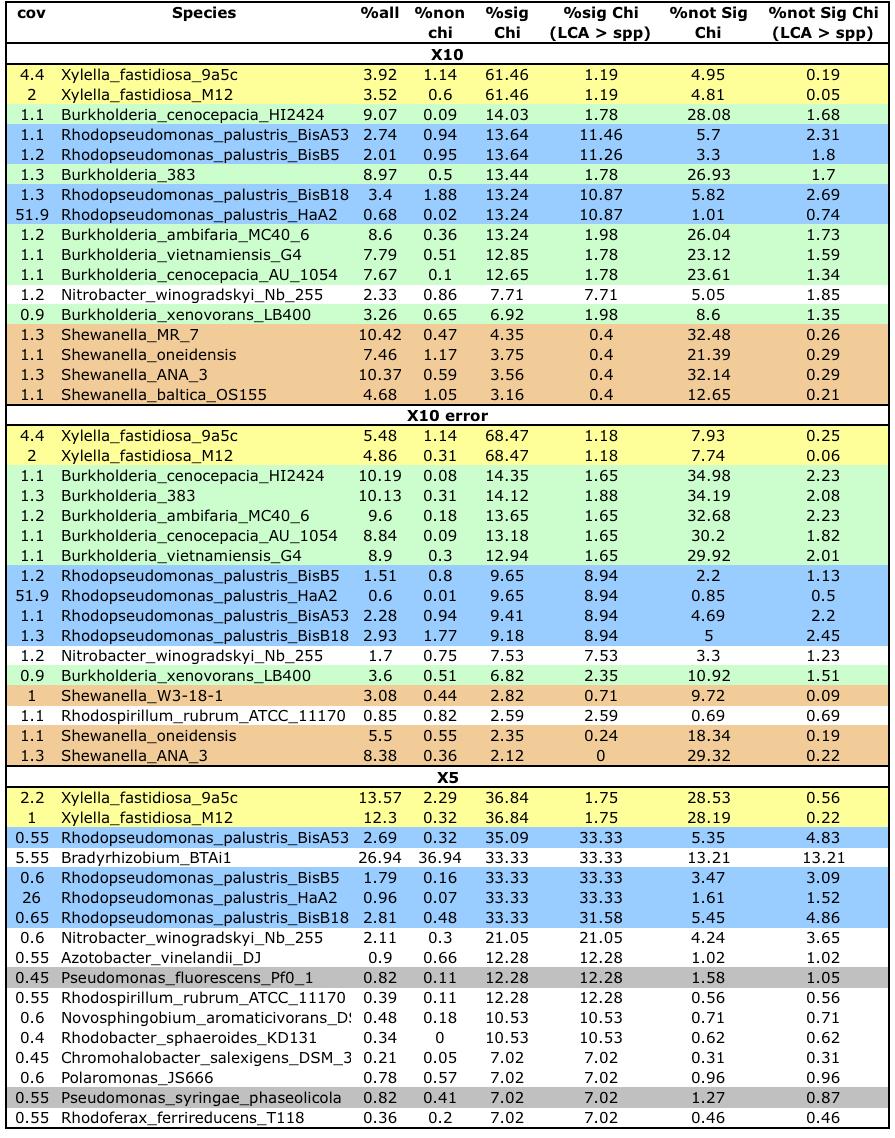
68 57