Section 5 The Integration of SWMM and SLAMM

Transcription

1 Section 5 The Integration of SWMM and SLAMM Introduction...1 SWMM (The Storm Water Management Model)...2 SLAMM (The Source Loading and Management Model)...2 SLAMM/SWMM Interface...3 SWMM, The EPA s Storm Water Management Model...3 RUNOFF Block...5 Pollutant Load Simulation...8 Other Capabilities and Summary...11 TRANSPORT Block...11 Flow Routing...12 Pollutant Routing...16 Other Capabilities and Summary...18 EXTRAN Block...18 STORAGE/TREATMENT Block...21 SLAMM, the Source Loading and Management Model...24 Introduction...24 History of SLAMM and Typical Uses...25 SLAMM Computational Processes...26 Monte Carlo Simulation of Pollutants Strengths Associated with Runoff from Various Urban Source Areas.30 Use of SLAMM to Identify Pollutant Sources and to Evaluate Different Control Programs...30 SLAMM/SWMM Interface Program...47 Introduction...47 SSIP Version SSIP Version How SSIP Works...48 Interface Program Instructions...48 Limitations and Caveats...49 Future Versions...49 References...49 Introduction The use of computers has become common in many aspects of engineering practice, including wet weather management. In fact, no reasonable methodology can be conducted without the analytical and modeling capabilities of a computer. Unfortunately, no currently available software package adequately integrates wet weather quantity and quality objectives. This project will, however, develop such a package with the integration of two currently used computer models -- the EPA s Storm Water Management Model (SWMM) (Huber, et al. 1988) and the Source Loading and Management Model (SLAMM) (Pitt and Voorhees 1995). These two popular models have unique characteristics that when merged will create the kind of tool needed for effective wet weather management. The integrated model will form the principal analytical tool used in the design methodology. 5-1

2 SWMM (The Storm Water Management Model) The U.S. Environmental Protection Agency s Storm Water Management Model (SWMM) is a large and relatively complex software package capable of simulating the movement of precipitation and pollutants from the ground surface, through pipe/channel networks and storage/treatment facilities, and finally to receiving waters. The model can be used to simulate a single event or a long, continuous period. SWMM is probably the most popular of all urban runoff models. Unfortunately, it has a reputation for being a difficult model to use. This is not necessarily the case if one knows the fundamentals of how it works and if the parts of the model not needed in a particular application are simply not used. SWMM uses well-known hydrologic and hydraulic concepts to simulate the urban drainage system. Its reputation for sophistication (and difficulty) derives more from the numerical algorithms necessary to solve the rather straightforward governing equations that are trying to simulate a complex system (i.e., the urban stormwater drainage system) driven by a highly dynamic input (i.e., precipitation). SWMM is divided into several blocks. The major blocks, i.e., RUNOFF, TRANSPORT, EXTRAN, and STORAGE/REATMENT are computational blocks responsible for the hydrologic, pollutant generation and transport, and hydraulic calculations. Others, i.e., EXECUTIVE, STATISTICAL, RAIN, TEMP, GRAPH, and COMBINE, perform various auxiliary functions, and are known as service blocks. The ability of SWMM to route flows and pollutants through a drainage and/or sewer system is its strength. While not very user friendly, it is not overly difficult to manage and use. A few preprocessing packages are available to help prepare the input data. SWMM is described later in this section, although because of the great deal of technical literature available for SWMM, the description is brief. SLAMM (The Source Loading and Management Model) SLAMM was originally developed to better understand the relationships between sources of urban runoff pollutants and runoff quality. It has been continually expanded since the late 1970s and now includes a wide variety of source area and outfall control practices (infiltration practices, wet detention ponds, porous pavement, street cleaning, catchbasin cleaning, and grass swales). SLAMM is strongly based on actual field observations, with minimal reliance on theoretical processes that have not been adequately documented or confirmed in the field. SLAMM is mostly used as a planning tool, to better understand sources of urban runoff pollutants and their control. Special emphasis has been placed on small storm hydrology and particulate washoff in SLAMM. Many currently available urban runoff models have their roots in drainage design where the emphasis is with very large and rare rains. In contrast, many stormwater quality problems are mostly associated with common and relatively small rains. The assumptions and simplifications that are legitimately used with drainage design models are not appropriate for water quality models. SLAMM therefore incorporates unique process descriptions to more accurately predict the sources of runoff pollutants and flows for the storms of most interest in stormwater quality analyses. However, SLAMM can be effectively used in conjunction with hydraulic models (such as SWMM in this project) to incorporate the mutual benefits of water quality controls and drainage design. SLAMM has been used in many areas of North America and has been shown to accurately predict stormwater flows and pollutant characteristics for a broad range of rains, development characteris tics, and control practices. SLAMM is unique in many aspects. One of the most important aspects is its ability to consider many stormwater controls (affecting source areas, drainage systems, and outfalls) together, for a long series of rains. Another is its ability to accurately describe a drainage area in sufficient detail for water quality investigations, but without requiring a great deal of superfluous information that field studies have shown to be of little value in accurately predicting discharge results. SLAMM also applies stochastic analysis procedures to more accurately represent actual uncertainty in model input parameters in order to better predict the actual range of outfall conditions (especially pollutant concentrations). However, the main reason SLAMM was developed was because of errors contained in many existing urban runoff models. These errors were obvious when comparing actual field measurements to the solutions obtained from model algorithms. 5-2

3 SLAMM is described in more detail later in this section, and in the Appendices. SLAMM/SWMM Interface In this project, SLAMM is used in place of SWMM s RUNOFF Block to provide the runoff and pollutant loads for input into the TRANSPORT, EXTRAN, or STORAGE/TREATMENT Blocks of SWMM. This approach better accounts for small storm processes and adds greater flexibility in evaluating source area flow and pollutant controls. SWMM has a well-developed Windows-based interface. The output from SLAMM will be manipulated so that it is acceptable for SWMM. The principal manipulation is to convert the event volume and load into event hydrographs and pollutographs. Secondarily, the flows and loads must be assigned to various locations in the sewer system, or storage/treatment system, simulated by SWMM. SLAMM currently provides the following output, in a one line per event format: Event characteristic 1. Event number 2. Rain start date 3. Rain start time 4. Julian start date and time 5. Rain duration (hrs) 6. Rain interevent period (days) 7. Runoff duration (hrs) 8. Rain depth (in) 9. Runoff volume (ft 3 ) 10. Volumetric runoff coefficient (R v ) 11. Average flow (cfs) 12. Peak flow (cfs) 13. Suspended solids concentration (mg/l) 14. Suspended solids mass (pounds) The interface package developed for SLAMM-SWMM will include the following capabilities: Ability to develop alternative hydrograph shapes for SLAMM runoff events. Assignment of source area hydrographs and pollutographs to specific locations on a sewer system or storage/treatment system simulated by SWMM. Ability to create a long time series of flows and loads from SLAMM (including dry periods) for effective long-term continuous simulation in SWMM. The SLAMM/SWMM Interface program will be Windows-based, programmed using Visual Basic. The most current public domain versions of SLAMM (version 8.4) and SWMM (version 4.4) will be used. SWMM, The EPA s Storm Water Management Model The U.S. Environmental Protection Agency Storm Water Management Model - or SWMM - is a large, relatively complex software package capable of simulating the movement of precipitation and pollutants from the ground surface, through pipe/channel networks and storage/treatment facilities, and finally to receiving waters. The model is can be used to simulate a single event or a long, continuous period. This summary is taken from a book by Nix (1994). SWMM has been released under several different official versions (Metcalf and Eddy, Inc., et al. 1971; Huber, et al. 1975, 1984; Huber and Dickinson, 1988; Roesner, et al. 1984, 1988) and there are many unofficial versions modified for specific purposes (some offered by private vendors). The original versions were designed for mainframe use, but the later versions can be executed on a personal computer. The current version of SWMM (Version 4.4; Huber and Dickinson, 1988 and Roesner, et al. 1988) may be obtained (along with the 5-3

4 documentation) from the Center for Exposure Assessment Modeling (CEAM), U.S. Environmental Protection Agency, College Station Road, Athens, Georgia The web site, from which the SWMM package can be downloaded, is ftp://ftp.epa.gov/epa_ceam/wwwhtml/ceamhome.htm. The CEAM phone number is SWMM is probably the most popular of all urban runoff models. Unfortunately, it has a reputation for being a difficult model to use. This is not necessarily the case if one knows the fundamentals of how it works and if the parts of the model not needed in a particular application are discarded. SWMM uses well-known hydrologic and hydraulic concepts to simulate the urban watershed. Its reputation for sophistication (and difficulty) derives more from the numerical algorithms necessary to solve the rather straightforward governing equations that are trying to simulate a complex system (i.e., the urban watershed) being driven by a highly dynamic input (i.e., precipitation). There is an extensive body of literature describing SWMM and a wide range of applications. Interested readers should begin their review of this literature by referring to a document prepared by Huber, et al. (1985). This large body of experience is an advantage that SWMM probably enjoys over all other urban runoff models. The SWMM internet user s group, through the University of Guelph, also offers a great deal of SWMM support. SWMM is divided into several blocks. The major blocks - i.e., RUNOFF, TRANSPORT, STORAGE/TREATMENT, and EXTRAN - are computational blocks responsible for the hydrologic, pollutant generation and transport, and hydraulic calculations. Others blocks - i.e., EXECUTIVE, STATISTICAL, RAIN, TEMP, GRAPH, and COMBINE - perform various auxiliary functions, and are known as service blocks. A general operational schematic of SWMM is shown in Figure 5-1. The computational blocks, RUNOFF, TRANSPORT, EXTRAN, and STORAGE/TREATMENT are described below. The RUNOFF Block is only summarized here so as to provide a comparison with SLAMM, recalling that SLAMM is replacing the RUNOFF Block. 5-4

5 Figure 5-1. SWMM, the Storm Water Management Model, program configuration (after Huber and Dickinson 1988). RUNOFF Block The RUNOFF Block generates surface runoff and pollutant loads in response to precipitation and surface pollutant accumulations (Huber and Dickinson, 1988). The key to applying RUNOFF is the division of the watershed into a number of subwatersheds (or subcatchments). Each subwatershed should be relatively homogeneous (i.e., the physical characteristics should be consistent). Just how homogeneous each subwatershed should be depends on how finely characterized the watershed must be to meet the modeling objectives. Dividing the watershed into a large number of subwatersheds implies that each is probably very homogeneous; a smaller number implies less homogeneity. Runoff Simulation. The conceptual view of surface runoff used by the RUNOFF Block is quite simple and is summarized in Figure 5-2. Essentially, each subwatershed surface is treated as a nonlinear reservoir with a single inflow precipitation. There are several discharges including infiltration, evaporation, and surface runoff. The capacity of this reservoir is the maximum depression storage, which is the maximum surface storage provided 5-5

6 by ponding, surface wetting, and interception. Surface runoff occurs only when the depth of water in the reservoir exceeds the maximum depression storage. Figure 5-2. Nonlinear reservoir representation of a subwatershed, RUNOFF Block, SWMM (Huber and Dickinson 1988). The water in storage is also being depleted by infiltration and evaporation. Infiltration occurs only if the ground surface is pervious (as opposed to an impervious surface, such as a paved parking lot, which by definition allows no infiltration). The infiltration process is modeled by one of two methods (Horton s equation or the Green-Ampt equation), which can be selected by the user. Infiltrated water is routed through upper and lower subsurface zones and may contribute to total runoff through ground water flow (this capability is a relatively new addition to SWMM). Monthly average evaporation rates (provided by the user) are directly employed to calculate the amount of water evaporated from the surface (and indirectly to calculate evapotranspiration from the subsurface zones). The precipitation intensity, less the rates of infiltration and evaporation, is known as the rainfall excess. The entire process is repeated for each subwatershed (each having its own unique set of physical characteristics) and is modeled by two equations. One is the continuity of mass equation, which tracks the volume or depth of water on the surface of the subwatershed: change in volume stored on the subwatershed per unit time rainfall excess(net inflow to the subwatershed) Runoff (outflow from the subwatershed) dv/dt = d(a d)/dt = (A i e ) - Q (5-1) where V = A d = volume of water on the subwatershed, feet 3 or meters 3 ; A = area of the subwatershed, feet 2 or meters 2 ; d = depth of water on the subwatershed, feet or meters; t = time, seconds; I e = rainfall excess, which is the rainfall intensity less the evaporation/infiltration rate, feet/second or meters/second; and Q = runoff flow rate from the subwatershed, feet 3 /second or meters 3 /second. 5-6

7 The second equation is based on Manning's equation and is used to model the rate of surface runoff (i.e., the outflow rate from the reservoir) as a function of the depth of flow above the maximum depression storage depth. Manning's equation can be stated as: Q = A c (β/n) R 2/3 S o 1/2 (5-2) where A c = cross-sectional area of flow over the subwatershed, feet 2 or meters 2 ; n = Manning's roughness coefficient; R = hydraulic radius of flow over the watershed, feet or meters; S o = slope of the subwatershed, feet/foot or meters/meter (which is assumed to equal the friction or energy slope); and β = 1.49 if U.S. customary units are used or 1.0 if metric units are used. The cross-sectional area of flow is: A c = W (d d p ) (5-3) where W = width of flow over the subwatershed, or the width of overland flow, feet or meters; and d p = depth of maximum depression storage, feet or meters. The hydraulic radius is the cross-sectional area of flow divided by the wetted perimeter. Since the depth of flow is very small, the wetted perimeter can be approximated by W. Thus, R can be calculated as: R = [W (d d p )]/W = d d p (5-4) Substituting Equations 5-3 and 5-4 into Equation 5-2 yields: Q = W (β/n) (d d p ) 5/3 S o 1/2 (5-5) Substituting Equation 5-5 into Equation 5-1 and dividing by A produces: dd/dt = i e - [(β W)/(A n)] (d d p ) 5/3 S o 1/2 (5-6) Equation 5-6 is the second governing equation used in RUNOFF. The two governing equations are solved numerically as follows. Equation 5-1 can be approximated by: (d n+1 -d n )/dt = i e Q/A (5-7) where t = t n+1 t n, time step size, seconds; n, n+1 = subscripts indicating conditions at the end of time step n (or start of time step n+1) and the end of time step n+1 (e.g., d n+1 is the depth at the end of time step n+1); i e = average precipitation intensity during time step n+1, feet/second or meters/second; and Q = average runoff flow rate during time step n+1, feet 3 /second or meters 3 /second. Equation 5-7 shows the differential term dd/dt approximated by a finite difference of values for depth at two points in time separated by t. The value of the differential term is then approximated by the average of the terms on the right-hand side evaluated at the beginning and end of t. If the average runoff flow rate is calculated as a function of the average depth of flow Equation 5-7 becomes: (d n+1 -d n )/dt = I e - [(β W)/(A n)] (d d p ) 5/3 S o 1/2 (5-8) where d = (d n + d n+1 )/2, average depth of flow during time step n+1, feet or meters. 5-7

8 Equation 5-8 is a relatively simple nonlinear, algebraic relationship with one unknown at any time, d n+1. (The value of d n is, of course, known from the end of the previous time step.) The Newton-Raphson technique for numerically solving a nonlinear equation is used to solve for d n+1. The calculated value of d n+1 is then used in Equation 5-5 to calculate the value of Q at the end of the time step. For all intents and purposes, Equation 5-8 is the core of the RUNOFF Block. The most perplexing parameter in Equation 5-8 is the width of overland flow, W. Essentially, it is the width over which surface runoff occurs. Again, using the reservoir analogy, this width is similar to the length of a weir or spillway. An idealized view is shown in Figure 5-3. In this schematic, surface runoff is being discharged to a drainage channel running down the center of the subwatershed. In this situation, the two halves are symmetrical and, thus, the total length of overland flow is twice the length of the channel. Of course, this idealized case never occurs, but it demonstrates the concept. The width of overland flow primarily affects the rapidity of runoff. Recall the weir analogy. In this case, though, when the weir width is enlarged, the length of the reservoir is shortened so that the surface area and depth of flow behind the weir remain constant for a given volume of water. As a result, a shorter width will delay runoff; a longer width will facilitate runoff. The RUNOFF Block has a limited ability to route flows through simple gutter and pipes using the nonlinear reservoir technique. However, the more sophisticated routines in TRANSPORT and EXTRAN Blocks are almost always employed for this purpose. The surface flows generated by the RUNOFF Block are concentrated at nodes. In other words, the flows are not distributed along gutters or pipes (as implied by Figure 5-3). The width of overland flow is used as a computational tool but the flow is not actually distributed over this distance. Pollutant Load Simulation The accumulation of pollutants on the subwatershed surface is modeled in a number of ways. Pollutants can be accumulated as dust and dirt on streets or as a simple areal load. Loads may be accumulated in a linear or nonlinear fashion. The different methods (essentially four different equations) are summarized in Figure 5-4 along with a visualization of the accumulation modeled by each. The washoff of accumulated pollutants is handled in one of two ways. One method applies the following firstorder relationship to each subwatershed: -P off = dp p /dt = -K P p (5-9) where P off = rate at which pollutant is washed off the subwatershed at time t, quantity/second; P p = amount of pollutant p on the subwatershed surface at time t, quantity; and K = coefficient, 1/second. 5-8

9 Figure 5-3. Idealized subwatershed-gutter arrangement illustrating the subwatershed width of overland flow, RUNOFF Block, SWMM (Huber and Dickinson 1988). 5-9

10 Figure 5-4. Buildup equations, RUNOFF Block, SWMM (after Huber and Dickinson 1988). The term quantity is used in the definitions of P off and P p because the pollutants modeled by SWMM can be characterized with a variety of units (e.g. milligrams, MPN for coliform bacteria, NTU for turbidity, etc.). Equation 5-9 says that the rate at which a pollutant disappears from a subwatershed surface is proportional to the amount remaining on the subwatershed surface. The coefficient K is assumed to be proportional to the runoff rate: K = R c r (5-10) where R c = washoff coefficient, inches -1 or millimeters -1 ; and r = runoff rate over the subwatershed at time t, inches/second or millimeters/second (calculated from Q in Equation 5-5, r = Q/A). Substituting Equation 5-10 into Equation 5-9 and multiplying by -1 yields: P off = -dp p /dt = R c r P p (5-11) A major deficiency of Equation 5-11 is that the runoff pollutant concentrations are forced to decrease over the course of a runoff event. Equation 5-11 shows the washoff rate increasing with runoff, but dividing Equation 5-11 by the runoff flow, Q, yields: C = P off /Q = conv(r c r P p )/(A r) = conv(r c P p )/A (5-12) 5-10

11 where C = concentration, quantity/volume; Q = A r, runoff flow rate, feet 3 /second or meters 3 /second; A = subwatershed area, acres or hectares; and conv = a constant containing a number of conversion factors. Note that the runoff rate, r, disappears in Equation Thus, the concentration, C, become independent of the runoff rate and directly proportional to a decreasing amount of pollutant remaining on the watershed. A decreasing concentration, while fairly common, is certainly not the only possible trend. Concentrations can increase during a runoff event. To overcome this problem, an exponent other than one is allowed for r: P off = -dp p /dt = R c r n P p (5-13) where n = exponent for the runoff rate. The load calculated by Equation 5-13 is combined with the runoff flow rate to calculate the concentration, i.e., C = P off /Q. If n = 1, Equation 5-13 reverts to Equation 11 and the concentration will decrease over the course of an event. Otherwise, concentration is proportional to r n-1 (recall Equation 5-12) and as such it may increase if the runoff rate is large enough to offset the reduced value of P p. The solution to Equation 5-13 is determined from a finite difference approximation which produces: P p (t+ t) = P p (t) exp{-r c 0.5 [r(t) n + r(t+ t) n ] t} (5-14) where 0.5[r(t) n + r(t+ t) n ] = average runoff rate over t, inches/second or millimeters/second. The second method allows the user to simulate the washoff as a simple function of the runoff rate: P off = R c Q n (5-15) where coefficients R c and n are assigned particular values for each pollutant. In this method, the simulation of pollutant load washoff may be totally independent of the amount accumulated on the surface (i.e., the load is a function of the runoff flow rate only) or may be linked to the accumulated amount by not allowing the total load discharged during a particular storm to exceed the amount present on the surface at the beginning of the storm. Other Capabilities and Summary There are many other capabilities not discussed here, most notably snowmelt simulation. The RUNOFF Block consumes a considerable portion of the SWMM user s manual, making it seem more profound and difficult than it is. Recall that the heart of the block is a very simple nonlinear reservoir representation of the surface runoff process, rudimentary nonlinear and linear buildup relationships, and a first-order washoff process. Unfortunately, many users incorrectly use RUNOFF through misinterpretation of the early stormwater data that was used in its development, especially the washoff mechanisms and infiltration of water through compacted soils and infiltration through pavement. In addition, RUNOFF doesn t allow direct application of many common stormwater control practices. For these reasons, SLAMM is used during this project to replace the RUNOFF block of SWMM. TRANSPORT Block The TRANSPORT Block routes flows and pollutant loads through a sewer system (Metcalf and Eddy, Inc., et al. 1971; Huber and Dickinson 1988). These flows and loads are generated by the RUNOFF Block (or some other program, e.g., SLAMM) and input to points throughout the system. TRANSPORT also has the ability to simulate dry-weather or sanitary sewage flows for routing through a sewer system. Hydrographs and pollutographs can also be manually introduced at various points in the system. 5-11

12 The sewer system is viewed as a series of elements. This is shown in Figure 5-5. Elements may be nodes or conduits. Nodes link conduits and include manholes, pump stations, storage units, and flow dividers (see Table 5-1). Inflows to the system, such as surface runoff, occur at the nodes and may be entered directly by the user or come from other programs such as the RUNOFF Block or SLAMM through an interface file. A conduit may have one of 15 different cross-sectional shapes supplied by the model or two supplied by the user (see Table 5-1). Simple flow diversion devices (e.g., overflow structures) are also allowed. Each element is identified by a user-supplied number. The numbering scheme can be arbitrary, for the system elements are fashioned into a connected network by indicating which elements are upstream of each element. In other words, element 11 is not necessarily connected to element 12, nor is element 12 necessarily connected to element 13. But element 119 can be connected to element 1034 if the user specifies that element 1034 is one of the elements immediately upstream of element 119. Flow Routing Ideally, flow in sewers can be represented by two partial differential equations: the continuity and momentum equations or, as they are sometimes known, the Saint-Venant equations (Chow, et al. 1988): Momentum: pressure force Convective Acceleration local acceleration gravity force friction force δh/δt + (v/g) δv/δx + (1/g) δv/δt = S o - S f (5-16) Continuity: inflows and outflows to and from a control volume change in amount of water in control volume δq/δx + δa/δt = 0 (5-17) where h = water depth, feet or meters; v = average flow velocity, feet/second or meters/second; x = distance along the conduit, feet or meters; t = time, seconds; g = acceleration due to gravity, 32.2 feet/second 2 or 9.8 meters/seconds 2 ; S o = invert slope (slope of the conduit), feet/foot or meters/meter; S f = friction (energy) slope, feet/foot or meters/meter; Q = flow rate, feet 3 /second or meters 3 /second; and A = cross-sectional area of flow, feet 2 or meters 2. Unfortunately, the Saint-Venant equations are difficult to manipulate and simplifications are often desirable. TRANSPORT uses a simplified version of the momentum equation in which all terms on the left hand side are neglected, i.e., S f = S o (5-18) 5-12

13 Figure 5-5. Node and conduit representation of a sewer system, TRANSPORT Block, SWMM (Heaney, et al. 1975). Table 5-1. Elements in TRANSPORT Block, SWMM (Huber and Dickinson 1988) 5-13

14 5-14

15 The friction slope, S f, is estimated from Manning s equation: S f = Q 2 /[(β/n) 2 A 2 R 4/3 ] (5-19) where n = Manning's roughness coefficient; R = hydraulic radius, feet or meters; and β = 1.49 when U.S. customary units are used or 1.0 when metric units are used. From Equations 5-18 and 5-19, Q = (k/n) A R 2/3 S o 1/2 (5-20) Essentially the original momentum equation, Equation 5-16, is replaced with an equation where Q is a function of depth only (recall that the cross-sectional area, A, and the hydraulic radius, R, are functions of depth, h). This kinematic wave approximation, as it is commonly known, is what distinguishes the TRANSPORT Block from its more sophisticated cousin, the EXTRAN Block (see the next section). Since flow is a function of depth alone, disturbances or changes that occur at one point in a sewer system can only affect what happens at downstream points, not upstream points. The full momentum equation propagates the effects of disturbances in both directions since flow (or velocity) is also a function of local and convective acceleration and pressure. With hydraulic effects propagated in only the downstream direction, backwater conditions cannot be simulated. In addition, the fact that flow is treated as a function of only depth means that the TRANSPORT Block cannot simulate surcharge conditions (flow under pressure). In summary, the TRANSPORT Block views the system as a simple cascade of conduits with downstream conduits having no effect on upstream conduits. It is especially important to understand how the TRANSPORT Block behaves when it encounters surcharge conditions. Flows exceeding the open-channel capacity of a conduit are stored at the upstream end of the conduit (at a node) and released when this capacity again becomes available. Hydrographs passing through such a conduit become clipped (as shown in Figure 5-6) and, as a result, potential surcharge problems at downstream conduits may be masked. The continuity equation, Equation 5-17, is approximated by a finite difference relationship: [(1-w t )(A j,n+1 - A j,n ) + w t (A j+1,n+1 - A j+1,n )]/ t + [(1-w x )(Q j+1,n Q j,n ) + w x (Q j+1,n+1 - Q j,n+1 )]/ x = 0 (5-21) where t = t n+1 - t n, time step size, seconds; x = x j+1 - x j, distance interval length (the conduit length), feet or meters; j, j+1 = subscripts indicating conditions at the upstream end and the downstream end of conduit M, respectively; n, n+1 = subscripts indicating conditions at the end of time step n (which is also the beginning of time step n+1) and the end of time step n+1, respectively; and w t, w x = weights. The weights w x and w t were both set to 0.55 after a series of tests to determine the best values for numerical stability. This numerical approximation and its application are illustrated in Figure 5-7. Equations 5-20 and 5-21 are used together to route flows through a sewer system. At the end of any time step n+1, the unknown quantities are the flow and cross-sectional area of flow at the downstream end of conduit M, Q j+1,n+1 and A j+1,n+1. (The variables Q j,n and A j,n are known from the previous time step and conditions at the upstream end of the conduit). With only two unknowns, these two equations are sufficient to determine the 5-15

16 Figure 5-6. Effect of surcharging on downstream hydrograph, TRANSPORT Block, SWMM. value of both. The calculations are carried out from the most upstream conduit to the most downstream conduit during each time step. Nodes (e.g., manholes) are treated very simply in the TRANSPORT Block. Flow exiting a node is just the sum of all the flows entering the node. Although the numbering scheme used to identify the various elements is arbitrary from the user's perspective, the program establishes a separate internal numbering scheme for the routing calculations. Again, this is possible because the user identifies the elements upstream of each element. It should be noted that several modifications were made to Equations 5-20 and 5-21 to improve model accuracy. These will not be discussed here. It is sufficient to say that these two equations are the heart of the TRANSPORT Block. Pollutant Routing Pollutants are routed through the system by treating each conduit as a completely mixed reactor with first-order decay. The governing differential equation is shown below: change in mass in conduit per unit time mass rate to conduit mass rate from conduit decay in conduit mass source or sink d(v C)/dt = V dc/dt + C dv/dt = (Q i C i ) - (Q C) - K C V ± L (5-22) 5-16

17 Figure 5-7. Numerical approximation definitions in TRANSPORT Block, SWMM (Metcalf and Eddy, Inc., et al. 1971). 5-17

18 where C = pollutant concentration in conduit and discharge from conduit, quantity/volume (e.g., milligrams/liter); V = volume of water in conduit, feet 3 or meters 3 ; Q i = inflow rate to conduit, feet 3 /second or meters 3 /second; C i = pollutant concentration in inflow, quantity/volume; Q = outflow rate from conduit, feet 3 /second or meters 3 /second; K = first-order decay coefficient, seconds -1 ; and L = source (or sink) of pollutant to the conduit, quantity/time. An integrated form of the solution to this differential equation is used with a simple numerical technique to carry out the estimates for concentration in each conduit. Other Capabilities and Summary The TRANSPORT Block has a very simple routine to estimate infiltration into the sewer system. The routine is not very useful and the user can just as easily enter infiltration flows at various nodes in the system. Unfortunately, there is no direct way to generate sewer infiltration from the subsurface flows simulated in the RUNOFF Block. The TRANSPORT Block also contains a rather data-intensive routine for estimating dry-weather flows and pollutant loads (which would be useful in watersheds with combined sewer systems). The estimates are calculated as functions of land use, population, income levels, and a host of other factors. In summary, the TRANSPORT Block effectively routes flows and pollutants through a simple sewer system, as long as surcharging is not encountered. Unlike its companion the EXTRAN Block, TRANSPORT is capable of routing pollutants. It is numerically stable and relatively easy to apply. EXTRAN Block The EXTRAN Block exceeds the hydraulic capabilities of the TRANSPORT Block, but omits pollutant routing (Roesner, et al. 1988). The block has a developmental history that is a little different from the rest of SWMM, joining the software bundle in the latter versions. Flow Routing. Similar to the TRANSPORT Block, the sewer system is viewed as a network of links and nodes (or, collectively, elements). Inflows to the system occur at the nodes and may be entered directly by the user or come from the RUNOFF Block or other programs (e.g., SLAMM). The number of element types that can be modeled is not as extensive as that of the TRANSPORT Block and the method of linking the system together is slightly different (see Table 5-2). Because hydraulic signals are propagated in both directions, upstream and downstream nodes are identified for each link (or conduit). The EXTRAN Block uses the complete Saint-Venant equations to model the routing of flows through a sewer system. However, the equations are expressed a little differently than in the previous section outlining the TRANSPORT Block (i.e., Equations 5-16 and 5-17): Momentum: pressure and gravity force convective acceleration local acceleration friction force g A (δh/δx) + δ(q 2 /A)/δx + δq/δt + g A S f = 0 (5-23) 5-18

19 Table 5-2. Elements in EXTRAN Block, SWMM (Roesner, et al. 1988) Continuity: inflows and outflows to and from a control volume change in amount of water in control volume δq/δx + δa/δt = 0 (5-24) 5-19

20 where H = z + h, hydraulic head, feet or meters; z = conduit invert elevation, feet or meters; h = water depth, feet or meters; x = distance along the conduit, feet or meters; t = time, seconds; g = acceleration due to gravity, 32.2 feet/second 2 or 9.8 meters/seconds 2 ; S f = friction (energy) slope, feet/foot or meters/meter; Q = flow rate, feet 3 /second or meters 3 /second; and A = cross-sectional area of flow, feet 2 or meters 2. Note that the gravity force term found in Equation 5-16 is incorporated in the first term of Equation The friction force term is estimated by Manning's equation: S f = Q 2 /[(β/n) 2 A 2 R 4/3 ] = Q v /[(β/n) 2 A 2 R 4/3 ] (5-25) where n = Manning s roughness coefficient; R = hydraulic radius, feet or meters; and β = 1.49 when U.S. customary units are used or 1.0 when metric units are used. The absolute value sign on velocity, v, insures that the friction force, as expressed by S f, opposes the direction of flow. For example, if flow is reversed (from the nominal direction of flow) both Q and v would be negative. Taking the absolute value of v allows S f to become negative as well. Equations 5-23 and 5-24 are combined through a few algebraic manipulations. These first of these relies on the identity Q 2 /A = v 2 /A (5-26) where v = average flow velocity, feet/second or meters/second. Substituting Equation 5-26 into the convective acceleration term of the momentum equation (Equation 5-23) yields: g A (δh/δx) + 2A v (δv/δx) + v 2 (δa/δx) + δq/δt + g A S f = 0 (5-27) Noting that Q = A v, the continuity equation, Equation 5-24, can be written as: A (δv/δx) + v (δa/δx) + δa/δt = 0 (5-28) Multiplying by velocity v and rearranging terms yields: A v (δv/δx) = -v (δa/δt) - v 2 (δa/δx) (5-29) Substituting this result into the second term of the revised momentum equation (Equation 5-27) leads to the basic flow equation used in the EXTRAN Block: g A (δh/δx) - 2v (δa/δt) - v 2 (δa/δx) + δq/δt + g A S f = 0 (5-30) Essentially, Equation 5-30 contains two variables, Q and H (v and A are related to Q and H). Therefore, the continuity equation (Equation 5-24) is used to provide a second equation relating Q and H at each node. Finite difference approximations are used to numerically solve the two partial differential equations. The details will not be discussed here. The numerical techniques used in the EXTRAN Block are somewhat unstable and some attention must be paid to the size of the time step and conduit lengths. 5-20

21 Other Capabilities and Summary. The routing of pollutant loads is not modeled. Nor are there routines for estimating sewer infiltration or dry-weather flows. The EXTRAN Block should be used with care and not undertaken lightly. While hydraulically powerful, it has proven to be numerically temperamental. Nevertheless, EXTRAN should be used if the sewer system to be modeled is complicated and subject to surcharging. STORAGE/TREATMENT Block The STORAGE/TREATMENT Block is designed to route flow and pollutant loads through a storage/treatment facility (Nix 1982; Huber and Dickinson 1988). These flows and loads may come from other blocks in SWMM or other sources. The user is given a great deal of flexibility by the block s ability to connect as many as five storage/treatment units together in a variety of networks. Each unit may be given detention (or storage) characteristics or be modeled as a simple flow-through device. If a unit is modeled as a detention unit, as shown in Figure 5-8, flows are routed through the unit with a level-surface flow routing procedure (i.e., the modified Puls method). This method is based on yet another version of the continuity of mass equation (Viessman, et al. 1988): change in volume of water in detention unit per unit time flow rate entering the detention unit flow rate leaving the detention unit dv/dt = I - Q (5-31) where V = volume of water in detention unit, feet 3 or meters 3 ; I = inflow rate, feet 3 /second or meters 3 /second; Q = outflow rate, feet 3 /second or meters 3 /second; and t = time, seconds. Equation 5-31 is approximated by the following finite difference relationship: (V n+1 V n )/ t = (I n + I n+1 )/2 + (Q n + Q n+1 )/2 (5-32) where n, n+1 = subscripts indicating conditions at the end of time step n (or the beginning of time step n+1) and the end of time step n+1, respectively; and t = t n+1 t n, time step size, seconds. At the end of any time step, the values of V n+1 and Q n+1 are unknown. (The values for V n and Q n are known from the previous time step.) A second relationship between storage, V, and discharge, Q, is needed to determine their values. The program gives the user a two ways to provide this relationship. One uses a linear interpolation algorithm to approximate the relationship through a series of volume-discharge data pairs (each pair occurring at a particular depth). With two relationships (Equation 5-32 and the user-supplied volume-discharge information) it is possible to solve for V n+1 and Q n+1 at each time step. Pollutants are routed through the detention unit in either a completely mixed or plug-flow manner. In the completely mixed case, all incoming material is instantly distributed throughout the detention unit and, thus, the pollutant concentration is uniform throughout the unit (see Figure 5-9). The following continuity of mass equation is used to simulate the fate of pollutants in the completely mixed detention unit: 5-21

22 Figure 5-8. Level-surface reservoir, STORAGE/TREATMENT Block, SWMM (after Huber and Dickinson 1988). change in mass in detention unit per unit time mass rate entering the detention unit mass rate leaving the detention unit reaction of pollutant by firstorder decay d(cv)/dt = I C I - Q C - K c C V (5-33) where C I = influent pollutant concentration, quantity/volume (e.g., milligrams/liter); C = effluent pollutant concentration, quantity/volume; and K c = decay coefficient, seconds -1. Equation 5-33 is approximated by a finite difference equation in a manner very similar to that done for Equation The result is an algebraic solution for the effluent pollutant concentration at the end of every time step. In the plug-flow case, the stormwater and pollutants entering the detention unit in a given time step forms a plug (see Figure 5-10). The number of plugs (and/or fraction of a plug) leaving the unit in any time step is, of course, directly related to the departing volume (as determined by the flow routing procedure). Pollutant removal is modeled through the use of removal equations or through a set of relationships describing discrete particle settling. In the former the program provides several variables such as detention time, inflow rate, etc. around which the user can build a wide range of removal equations. This is done by providing a generic function that can be manipulated through the assignment of the program variables to the variables in the generic equation and the selection of appropriate values for the equation coefficients. The generic function is: R = [a 12 exp(a 1 x 1 ) x 2 a2 + a 13 exp(a 3 x 3 ) x 4 a4 + a 14 exp(a 5 x 5 ) x 6 a6 + a 15 exp(a 7 x 7 +a 8 x 8 ) x 9 a9 x 10 a10 x 11 a11 ] a16 (5-34) 5-22

23 Figure 5-9. Completely mixed detention unit, STORAGE/TREATMENT Block, SWMM (Huber and Dickinson 1988). Figure Plug-flow detention unit, STORAGE/TREATMENT Block, SWMM (Huber and Dickinson 1988). 5-23

24 where x i = removal equation variable; a j = coefficients; and R = removal fraction, 0 R 1.0. As mentioned above, each variable x i can represent one of a number of variables in the storage/treatment algorithm. The selection varies depending on whether the detention basin is assumed to behave as a plug-flow reactor or a completely mixed reactor. In the completely mixed mode, Equation 5-34 is really only used to provide a value for K c in Equation In the plug-flow mode, the equation is applied to each plug and many more options are available. The particle-settling algorithm can only be used in the plug-flow mode. The size distribution of particles entering the detention unit is assumed to remain constant for all incoming flows. The settling of particles is based on the theory of discrete particle settling modified for the effects of turbulence (Nix 1982). The outgoing size distribution changes over time as differences in flow conditions dictate. The removal (settling) of a particular pollutant is based on its association with particles of various settling velocities or sizes and specific gravities (e.g., 20% of the BOD load is associated with particles that have a given range of settling velocities). This association also remains constant for all incoming pollutant loads. This assumption, and that of a constant particle size distribution, is a major limitation. It should be said, however, that this limitation only exists because the RUNOFF Block does not predict the distribution of particle sizes carried along with stormwater runoff. The algorithms in the STORAGE/TREATMENT Block can handle time-varying distributions. When a unit is defined as a simple flow-through or non-detention device, flow is routed without delay, i.e., inflow = outflow. Pollutant removal is simulated with Equation 5-34 (again, built by the user with variables provided by the program), or by assuming that all particles of a certain size or larger are removed. The STORAGE/TREATMENT Block is not intended to be a sophisticated unit operations simulator. There are other models that simulate these processes in great detail. This block is designed to give the user a reasonable prediction of how a wet-weather facility will respond to dynamic stormwater flows and pollutant loads. In order to keep the model tractable, the representation of pollutant routing and removal is fairly simple. SLAMM, the Source Loading and Management Model Introduction The Source Loading and Management Model (SLAMM) was originally developed to better understand the relationships between sources of urban runoff pollutants and runoff quality. It has been continually expanded since the late 1970s and now includes a wide variety of source area and outfall control practices (infiltration practices, wet detention ponds, porous pavement, street cleaning, catchbasin cleaning, and grass swales). SLAMM is strongly based on actual field observations, with minimal reliance on pure theoretical processes that have not been adequately documented or confirmed in the field. SLAMM is mostly used as a planning tool, to better understand sources of urban runoff pollutants and their control. Special emphasis has been placed on small storm hydrology and particulate washoff in SLAMM, common areas of misuse in the SWMM RUNOFF block. Many currently available urban runoff models have their roots in drainage design where the emphasis is with very large and rare rains. In contrast, stormwater quality problems are mostly associated with common and relatively small rains. The assumptions and simplifications that are legitimately used with drainage design models are not appropriate for water quality models. SLAMM therefore incorporates unique process descriptions to more accurately predict the sources of runoff pollutants and flows for the storms of most interest in stormwater quality analyses. However, SLAMM can be effectively used in conjunction with drainage design models to incorporate the mutual benefits of water quality controls on drainage design. SLAMM has been used in many areas of North America and has been shown to accurately predict stormwater flows and pollutant characteristics for a broad range of rains, development characteristics, and control practices. As with all 5-24

25 stormwater models, SLAMM needs to be accurately calibrated and then tested (verified) as part of any local stormwater management effort. SLAMM is unique in many aspects. One of the most important aspects is its ability to consider many stormwater controls (affecting source areas, drainage systems, and outfalls) together, for a long series of rains. Another is its ability to accurately describe a drainage area in sufficient detail for water quality investigations, but without requiring a great deal of superfluous information that field studies have shown to be of little value in accurately predicting discharge results. SLAMM also applies stochastic analysis procedures to more accurately represent actual uncertainty in model input parameters in order to better predict the actual range of outfall conditions (especially pollutant concentrations). However, the main reason SLAMM was developed was because of errors contained in many existing urban runoff models. These errors were obvious when comparing actual field measurements to the solutions obtained from model algorithms. In addition to the material presented in this report section, Appendices A and B summarize the small storm hydrology features used in SLAMM (showing how drainage and water quality objectives can be both addressed with the model), Appendix C is a user s guide for using SLAMM, Appendix D describes the source area and outfall controls incorporated in SLAMM, and Appendix E contains the source code for SLAMM. History of SLAMM and Typical Uses The Source Loading and Management Model (SLAMM) was initially developed to more efficiently evaluate stormwater control practices. It soon became evident that in order to accurately evaluate the effectiveness of stormwater controls at an outfall, the sources of the pollutants or problem water flows must be known. SLAMM has evolved to include a variety of source area and end-of-pipe controls and the ability to predict the concentrations and loadings of many different pollutants from a large number of potential source areas. SLAMM calculates mass balances for both particulate and dissolved pollutants and runoff flow volumes for different development characteristics and rainfalls. It was designed to give relatively simple answers (pollutant mass discharges and control measure effects for a very large variety of potential conditions). SLAMM was developed primarily as a planning level tool, such as to generate information needed to make planning level decisions, while not generating or requiring superfluous information. Its primary capabilities include predicting flow and pollutant discharges that reflect a broad variety of development conditions and the use of many combinations of common urban runoff control practices. Control practices evaluated by SLAMM include detention ponds, infiltration devices, porous pavements, grass swales, catchbasin cleaning, and street cleaning. These controls can be evaluated in many combinations and at many source areas as well as the outfall location. SLAMM also predicts the relative contributions of different source areas (roofs, streets, parking areas, landscaped areas, undeveloped areas, etc.) for each land use investigated. As an aid in designing urban drainage systems, SLAMM also calculates correct NRCS curve numbers that reflect specific development and control characteristics. These curve numbers can then be used in conjunction with available urban drainage procedures to reflect the water quantity reduction benefits of stormwater quality controls. SLAMM is normally used to predict source area contributions and outfall discharges. However, SLAMM has been used in conjunction with a receiving water model (HSPF) to examine the ultimate receiving water effects of urban runoff (Ontario 1986). The development of SLAMM began in the mid 1970s, primarily as a data reduction tool for use in early street cleaning and pollutant source identification projects sponsored by the EPA s Storm and Combined Sewer Pollution Control Program (Pitt 1979; Pitt and Bozeman 1982; Pitt 1984). Additional information contained in SLAMM was obtained during the EPA s Nationwide Urban Runoff Program (NURP) (EPA 1983), especially the early Alameda County, California (Pitt and Shawley 1982), and the Bellevue, Washington (Pitt and Bissonnette 1984) projects. The completion of the model was made possible by the remainder of the NURP projects and additional field studies and programming support sponsored by the Ontario Ministry of the Environment (Pitt and McLean 1986), the Wisconsin Department of Natural Resources (Pitt 1986), and Region V of the U.S. Environmental Protection Agency. Early users 5-25

26 of SLAMM included the Ontario Ministry of the Environment s Toronto Area Watershed Management Strategy (TAWMS) study (Pitt and McLean 1986) and the Wisconsin Department of Natural Resources Priority Watershed Program (Pitt 1986). SLAMM can now be effectively used as a tool to enable watershed planners to obtain a better understanding of the effectiveness of different control practice programs. A logical approach to stormwater management requires knowledge of the problems that are to be solved, the sources of the problem pollutants, and the effectiveness of stormwater management practices that can control the problem pollutants at their sources and at outfalls. SLAMM is designed to provide information on these last two aspects of this approach. SLAMM Computational Processes Figure 5-11 illustrates the wide variety of development characteristics that affect stormwater quality and quantity. This figure shows a variety of drainage systems from concrete curb and gutters to grass swales, along with directly connected roof drainage systems and drainage systems that drain to pervious areas. Development characteristics define the magnitude of these drainage efficiency attributes, along with the areas associated with each surface type (road surfaces, roofs, landscaped areas, etc.). The use of SLAMM shows that these characteristics greatly affect runoff quality and quantity. Land use alone is usually not sufficient to describe these characteristics. The types of the drainage system (curbs and gutters or grass swales) and roof connections (directly connected or draining to pervious area), are probably the most important attributes affecting runoff characteristics. These attributes are not directly related to land use, but some trends are obvious: most roofs in strip commercial and shopping center areas are directly connected, and the roadside is most likely drained by curbs and gutters, for example. Different land uses, of course, are also associated with different levels of pollutant generation. For example, industrial areas usually have the greatest pollutant accumulations due to material transfer and storage, and heavy truck traffic. Figure 5-12 shows how SLAMM considers a variety of pollutant and flow routings that may occur in urban areas. SLAMM routes material from unconnected sources to the drainage system directly or to adjacent directly connected or pervious areas which in turn drain to the collection system. Each of these areas has pollutant deposition mechanisms in addition to removal mechanisms associated with them. As an example, unconnected sources, which may include rooftops draining to pervious areas or bare ground and landscaped areas, are affected by regional air pollutant deposition (from point source emissions or from fugitive dust) and other aspects that would affect all surfaces. Pollutant losses from these unconnected sources are caused by wind removal and by rain runoff washoff which flow directly to the drainage system, or to adjacent areas. The drainage system may include curbs and gutters where there is limited deposition, and catch basins and grass swales which may remove substantial participates that are transported in the drainage system. Directly connected impervious areas include paved surfaces that drain directly to the drainage system. These source areas are also affected by regional pollutant deposition, in addition to wind removal and controlled removal processes, such as street cleaning. On-site storage is also important on paved surfaces because of the large amount of participate pollutants that are not washed-off, blown-off, or removed by direct cleaning (Pitt 1979; Pitt and Shawley 1982; Pitt 1984). Figure 5-13 shows how SLAMM proceeds through the major calculations. There is a double set of nested loops in the analyses where runoff volume and suspended solids (particulate residue) are calculated for each source area and then for each rain. These calculations consider the affects of each source area control, in addition to the runoff pattern between areas. Suspended solids washoff and runoff volume from each individual area for each rain are summed for the entire drainage system. The effects of the drainage system controls (catch basins or grass swales, for example) are then calculated. Finally, the effects of the outfall controls are calculated. SLAMM uses the water volume and suspended solids concentrations at the outfall to calculate the other pollutant concentrations and loadings. SLAMM keeps track of the portion of the total outfall suspended solids loading and runoff volume that originated from each source area. The suspended solids fractions are then used to develop 5-26

27 Figure Urban runoff source areas and drainage alternatives (Pitt 1986). 5-27

28 Figure Pollutant deposition and removal at source areas (Pitt 1986). 5-28

29 Figure SLAMM calculation flow chart. 5-29

30 weighted loading factors associated with each pollutant. In a similar manner, dissolved pollutant concentrations and loadings are calculated based on the percentage of water volume that originates from each of the source areas within the drainage system. SLAMM predicts urban runoff discharge parameters (total storm runoff flow volume, flow-weighted pollutant concentrations, and total storm pollutant yields) for many individual storms and for the complete study period. It has built-in Monte Carlo sampling procedures to consider many of the uncertainties common in model input values. This enables the model output to be expressed in probabilistic terms that more accurately represent the likely range of results expected. Monte Carlo Simulation of Pollutants Strengths Associated with Runoff from Various Urban Source Areas Initial versions of SLAMM only used average concentration factors for different land use areas and source areas. This was satisfactory for predicting the event mean concentrations (EMC, as used by NURP, EPA 1983) for an extended period of time and in calculating the unit area loadings for different land uses. Figure 5-14 is a plot of the event mean concentrations at a Toronto test sites (Pitt and McLean 1986). The observed concentrations are compared to the SLAMM predicted concentrations for a long term simulation. All of the predicted EMC values are very close to the observed EMC values. However, in order to predict the probability distributions of the concentrations, it was necessary to include probability information for the concentrations found in the different source areas. Statistical analyses of concentration data (attempting to relate concentration trends to rain depths and season, for example) from these different source areas have not been able to explain all of the variation in concentrations that have been observed. The statistical analyses also indicate that most pollutant concentration values from individual source areas are distributed log-normally. Therefore, log-normally distributed random concentration values are used in SLAMM for these different areas. The result is much more reasonable predictions for concentration distributions at the outfall when compared to actual observed conditions. This provides more accurate estimates of criteria violations for different stormwater pollutants at an outfall for long continuous simulations. Use of SLAMM to Identify Pollutant Sources and to Evaluate Different Control Programs Table 5-3 is a field sheet that has been developed to assist users of SLA MM describe test watershed areas. This sheet is mostly used to evaluate stormwater control retrofit practices in existing developed areas, and to examine how different new development standards effect runoff conditions. Much of the information on the sheet is not actually required to operate SLAMM, but is very important when considering additional control programs (such as public education and good housekeeping practices) that are not quantified by SLAMM. The most important information shown on this sheet is the land use, the type of the gutter or drainage system, and the method of drainage from roofs and large paved areas to the drainage system. The efficiency of drainage in an area, specifically if roof runoff or parking runoff drains across grass surfaces, can be very important when determining the amount of water and pollutants that enter the outfall system. Similarly, the presence of grass swales in an area may substantially reduce the amount of pollutants and water discharged. This information is therefore required to use SLAMM. The areas of the different surfaces in each land use is also very important for SLAMM. Figure 5-15 is an example showing the areas of different surfaces for a medium density residential area in Milwaukee. As shown in this examp le, streets make up between 10 and 20 percent of the total area, while landscaped areas can make up about half of the drainage area. The variation of these different surfaces can be very large within a designated area. The analysis of many candidate areas may therefore be necessary to understand how effective or how consistent the model results may be for a general land use classification. Tables 5-4 and Table 5-5 are coding sheets that have been prepared for SLAMM users. The information on these sheets is used by SLAMM to determine the concentrations and loadings from the different source areas and the effectiveness of different control practices. Table 5-4 shows general information describing the areas and the 5-30

31 Figure Observed and modeled outfall pollutant concentrations Emery (industrial site) (Pitt 1987). 5-31

32 Table 5-3. Study Area Description Field Sheet 5-32

33 Figure Source areas Milwaukee medium density residential areas (without alleys) (Pitt 1987). 5-33

34 Table 5-4a. SLAMM Site Characterization Data Coding Sheet (Pitt and Voorhees 1995) 5-34

35 Table 5-4b. SLAMM Site Characterization Data Coding Sheet (Pitt and Voorhees 1995) 5-35

36

37 Table 5-5a. SLAMM Control Device Data Sheet (Pitt and Voorhees 1995) 5-37

38 Table 5-5b. SLAMM Control Device Data Sheet (Pitt and Voorhees 1995) 5-38

39 Table 5-5c. SLAMM Control Device Data Sheet (Pitt and Voorhees 1995) 5-39

40 Table 5-5d. SLAMM Control Device Data Sheet (Pitt and Voorhees 1995) 5-40

41 characteristics of source areas. More information is required for some source areas than others, based upon responses to questions. Table 5-5 contains the coding sheets to describe the types of control practices that are to be investigated using SLAMM in a specific watershed area. Control practices evaluated by SLAMM include infiltration trenches, seepage pits, disconnections of directly connected roofs and paved areas, percolation ponds, street cleaning, porous pavements, catchbasin cleaning, grass swales, and wet detention ponds. These devices can be used singly or in combination, at source areas or at the outfalls or, in the case of grass swales and catchbasins, within the drainage system. In addition, SLAMM provides a great deal of flexibility in describing the sizes and other design aspects for these different practices. One of the first problems in evaluating an urban area for stormwater controls is the need to understand where the pollutants of concern are originating under different rain conditions. Figures 5-16 through 5-19 are examples for a typical medium density residential area (described in the previous coding sheets) showing the percentage of different pollutants originated from different major sources, as a function of rain depth. As an example, Figure 5-16 shows the areas where water is originating. For storms of up to about 0.1 inch in depth, street surfaces contribute about one-half to the total runoff to the outfall. This contribution decreased to about 20 percent for storms greater than about 0.25 inch in depth. This decrease in the significance of streets as a source of water is associated with an increase of water contributions from landscaped areas (which make up more than 75% of the area and have clayey soils). Similarly, the significance of runoff from driveways and roofs also starts off relatively high and then decreases with increasing storm depth. Figures 5-17, 5-18 and 5-19 are similar plots for suspended solids, phosphorus and lead. These show that streets contribute almost all of these pollutants for the smallest storms up to about 0.1 inch. The contributions from landscaped areas then become dominant. Figure 5-19 shows that the contributions of phosphates are more evenly distributed between streets, driveways, and rooftops for the small storms, but the contributions from landscaped areas completely dominate for storms greater than about 0.25 inch in depth. Obviously, these are just example plots and the source contributions would vary greatly for different land uses/development conditions, rainfall patterns, and the use of different source area controls. A major use of SLAMM is to better understand the role of different sources of pollutants. As an example, to control suspended solids, street cleaning (or any other method to reduce the washoff of particulates from streets) may be very effective for the smallest storms, but would have very little benefit for storms greater than about 0.25 inches in depth. However, erosion control from landscaped surfaces may be effective over a wider range of storms. The following list shows the different control programs that were investigated in this hypothetical medium density residential area having clayey soils: Base level (as built in with no additional controls) Catchbasin cleaning Street cleaning Grass swales Roof disconnections Wet detention pond Catchbasin and street cleaning combined Roof disconnections and grass swales combined All of the controls combined This residential area, which was based upon actual Birmingham, Alabama, field observations for homes built between 1961 to 1980, has no controls, including no street cleaning or catchbasin cleaning. The use of catchbasin cleaning in the area, in addition to street cleaning was evaluated. Grass swale use was also evaluated, but swales are an unlikely retrofit option, and would only be appropriate for newly developing areas. However, it is possible to disconnect some of the roof drainages and divert the roof runoff away from the drainage system and onto grass surfaces for infiltration in existing developments. In addition, wet detention ponds can be retrofitted in different areas and at outfalls. Besides those controls examined individually, catchbasin and street cleaning controls 5-41

42 Figure Flow sources for example medium density residential area having clayey soils (Pitt and Voorhees 1995). Figure 5-17 Suspended solids sources for example medium density residential area having clayey soils (Pitt and Voorhees 1995). 5-42

43 Figure 5-18 Total lead sources for example medium density residential area having clayey soils (Pitt and Voorhees 1995). Figure 5-19 Dissolved phosphate sources for example medium density residential area having clayey soils (Pitt and Voorhees 1995). 5-43

44 5-44

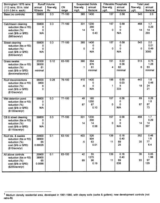
45 combined were also evaluated, in addition to the combination of disconnecting some of the rooftops and the use of grass swales. Finally, all of the controls together were also examined. The following list shows a general description of this hypothetical area: all curb and gutter drainage (in fair condition) 70% of roofs drain to landscaped areas 50% of driveways drain to lawns 90% of streets are intermediate texture (remaining are rough) no street cleaning no catchbasins About one-half of the driveways currently drain to landscaped areas, while the other half drain directly to the pavement or the drainage system. Almost all of the streets are of intermediate texture, and about 10 percent are rough textured. As noted earlier, there currently is no street cleaning or catchbasin cleaning. The level of catchbasin use that was investigated for this site included 950 ft 3 of total sump volume per 100 acres (typical for this land use), with a cost of about $50 per catchbasin cleaning. Typically, catch basins in this area could be cleaned about twice a year for a total annual cost of about $85 per acre of the watershed. Street cleaning could also be used with a monthly cleaning effort for about $30 per year per watershed acre. Light parking and no parking restrictions during cleaning is assumed, and the cleaning cost is estimated to be $80 per curb mile. Grass swale drainage was also investigated, assuming that swales could be used throughout the area, there could be 350 feet of swales per acre (typical for this land use), and the swales were 3.5 ft. wide. Because of the clayey soil conditions, an average infiltration rate of about 0.5 inch per hour was used in this analysis, based on many different double ring infiltrometer tests of typical soil conditions. Swales cost much less than conventional curb and gutter systems, but have an increased maintenance frequency. Again, the use of grass swales is appropriate for new development, but not for retrofitting in this area. Roof disconnections could also be utilized as a control measure by directing all roof drains to landscaped areas. The objective would be to direct all the roof drains to landscaped areas. Since 70 percent of the roofs already drain to the landscaped areas, only 30 percent could be further disconnected, at a cost of about $125 per household. The estimated total annual cost would be about $10 per watershed acre. An outfall wet detention pond suitable for 100 acres of this medium density residential area would have a wet pond surface of 0.5% of drainage area to provide about 90% suspended solids control. It would need 3 ft. of dead storage and live storage equal to runoff from 1.25 rain. A 90 o V notch weir and 5 ft. wide emergency spillway could be used. No seepage or evaporation was assumed. The total annual cost was estimated to be about $ 130 per watershed acre. Table 5-6 summarizes the SLAMM results for runoff volume, suspended solids, filterable phosphate, and total lead for 100 acres of this medium density residential area. The only control practices evaluated that would reduce runoff volume are the grass swales and roof disconnections. All of the other control practices evaluated do not infiltrate stormwater. Table 5-6 also shows the total annual average volumetric runoff coefficient (Rv) for these different options. The base level of control has an annual flow-weighted Rv of about 0.3, while the use of swales would reduce the Rv to about 0.1. Only a small reduction of Rv (less than 10 percent) would be associated with complete roof disconnections compared to the existing situation because of the large amount of roof disconnections that already occur. The suspended solids analyses shows that catchbasin cleaning alone could result in about 14 percent suspended solids reductions. Street cleaning would have very little benefit, while the use of grass swales would reduce the suspended solids discharges by about 60 percent. Grass swales would have minimal effect on the Table 5-6 SLAMM Predicted Runoff and Pollutant Discharge Conditions for Example 1 (Pitt and Voorhees 1995) 5-45

46 5-46