Structures and Dynamics in Live Bacteria Revealed by Super- Resolution Fluorescence Microscopy

Transcription

1 Structures and Dynamics in Live Bacteria Revealed by Super- Resolution Fluorescence Microscopy The Harvard community has made this article openly available. Please share how this access benefits you. Your story matters. Citation Accessed Citable Link Terms of Use Wang, Wenqin Structures and Dynamics in Live Bacteria Revealed by Super-Resolution Fluorescence Microscopy. Doctoral dissertation, Harvard University. December 16, :44:28 PM EST This article was downloaded from Harvard University's DASH repository, and is made available under the terms and conditions applicable to Other Posted Material, as set forth at (Article begins on next page)

2 c Wenqin Wang All rights reserved.

3 Thesis advisor Professor Xiaowei Zhuang Author Wenqin Wang Structures and dynamics in live bacteria revealed by super-resolution fluorescence microscopy Abstract Light microscopy, in particular fluorescence microscopy, is a widely used imaging method in biological research due to its noninvasive nature and molecular specificity. The resolution of conventional fluorescence microscopy is limited to a few hundred nanometers by the diffraction of light, leaving many biological structures too small to be optically resolved. Stochastic Optical Reconstruction Microscopy (STORM) technique overcomes this limit by localizing single photoswitchable fluorophores separated in time. We further extended the then two-dimensional capability to three-dimensional (3D) STORM by determining both axial and lateral positions of individual fluorophores with nanometer accuracy using optical astigmatism. Iterative, stochastic activation of photo-switchable probes enables high-precision 3D localization of each probe and thus the construction of a 3D image without scanning the sample. We achieved an image resolution of nm in the lateral dimensions and nm in the axial dimension. This development allowed us to resolve the 3D morphology of nanoscopic cellular structures. Enabled by the super-resolution imaging capability, we used 3D STORM in conjunction with biochemical assays to study structures and dynamics in live bacteria. iii

4 Abstract iv Bacterial chromosomes are confined in submicron-sized nucleoids. Chromosome organization is facilitated by nucleoid-associated proteins (NAPs), but the structure of the chromosome and the molecular mechanisms underlying its organization are poorly understood, in part due to the lack of appropriate tools for visualizing the chromosome in vivo. Using STORM, we found that four NAPs, HU, Fis, IHF, and StpA, were largely scattered throughout the E. coli nucleoid. In contrast, H-NS, a global transcriptional silencer, formed two compact clusters per chromosome driven by oligomerization of DNA-bound H-NS, through their N-terminal domain interactions. H-NS sequestered the regulated operons into these clusters and juxtaposed numerous DNA segments broadly distributed throughout the chromosome. Deleting H-NS led to substantial chromosome reorganization. These observations demonstrate that H-NS plays a key role in global chromosome organization in E. coli. Finally, we describe the use of the same sub-diffraction localization for singleparticle tracking to study MreB paralogs(actin-like proteins in bacteria) in B. subtilis. We found that MreB and the elongation machinery moved circumferentially around the cell, perpendicular to its length, with nearby synthesis complexes and MreB filaments moving independently in both directions. Inhibition of cell wall synthesis by various methods blocked the movement of MreB. Thus, bacteria elongate by the uncoordinated, circumferential movements of synthetic complexes that insert radial hoops of new peptidoglycan during their transit, possibly driving the motion of the underlying MreB filaments.

5 Contents Title Page Abstract Table of Contents Citations to Previously Published Work Acknowledgments i iii v vi vii 1 Introduction Introduction to fluorescence microscopy Diffraction-limited resolution Stochastic Optical Reconstruction Microscopy (STORM) Structure of this thesis Three-dimensional super-resolution imaging by Stochastic Optical Reconstruction Microscopy (3D STORM) Introduction Proof of principle, using optical astigmatism D STORM of microtubules and clathrin-coated pits Materials and methods Chromosome organization by a nucleoid-associated protein in live E. coli cells revealed by STORM Introduction Spatial distribution of major nucleoid-associated proteins H-NS clusters Colocalization of H-NS clusters and specific gene loci H-NS-regulated genes are brought into close proximity by H-NS v

6 Contents vi 3.6 Conclusions Materials and methods Coupled, circumferential motions of the cell wall synthesis machinery and MreB filaments in B. subtilis Introduction MreB paralogs display circumferential motion independent of the cell body Filament motion requires cell wall synthesis Single particle tracking of MreB paralogs and peptidoglycan elongation machinery (PGEM) Relative dynamics of MreB paralogs and PGEM Conclusions Materials and methods Conclusions and discussions Brief review of this thesis Discussions A 3D localization precision analysis of single fluorescence emitters 128 A.1 Localization precision in lateral dimensions (xy) A.2 Uncertainty of the image widths A.3 Localization precision in the axial direction (z) A.4 3D localization precisions: theory vs simulation Bibliography 151

7 Citations to Previously Published Work Portions of Chapters 1 and 2 have appeared in the following book chapter: G. Dempsey*, W. Wang*, X. Zhuang, Fluorescence imaging at subdiffraction limit resolution with stochastic optical reconstruction microscopy, Handbook of Single-Molecule Biophysics, Springer (2009) Large portions of Chapter 2 have appeared in the following paper: B. Huang, W. Wang, M. Bates, X. Zhuang, Three-dimension superresolution imaging by stochastic optical reconstruction microscopy, Science, 319: 810 (2008) Chapter 3 has been previously published with minor changes as the following paper: W. Wang*, G.W. Li*, C. Chen*, X. Xie, X. Zhuang, Chromosome organization by a nucleoid associated protein in live bacteria, Science, 333: 1445 (2011) Chapter 4 has been previously published with minor changes as the following paper: E. Garner, R. Bernard, W. Wang, X. Zhuang, D. Rudner, T. Mitchison, Circumferential motions of the cell wall synthesis machinery drives cytoskeletal dynamics in B. subtilis, Science, 333: 222 (2011) *: Equal-contribution authors vii

8 Acknowledgments This work would not have happened without many remarkable people. I have been very privileged to have their help and support. I would like to thank my advisor, Professor Xiaowei Zhuang, for her continued support and encouragement. Xiaowei s broad vision, tremendous scientific interest and extraordinary conviction have always guided my studies at Harvard. I am very grateful for her inspirational mentorship and insightful guidance. I would also like to thank Professor Sunney Xiaoliang Xie for close collaborations and advice on the E. coli chromosome orgnazation projects, Professor Richard Losick, Professor David Rudner, and Professor Aravinthan Samuel, for stimulating discussions and suggestions on our research projects in the large field of bacterial cell biology and biophysics. I have had the pleasure of collaborating with many incredible students and postdocs. First, I would like to thank Dr. Bo Huang for introducing me to the field of single-molecule microscopy, and being an amazing mentor, collaborator and friend. I would also like to thank Dr. James Kain and Dr. Kumaran Ramamurthi for introducing me to the beautiful bugs Bacillus subtilis. I would like to acknowledge Chongyi Chen and Dr. Gene-Wei Li, both of whom made important contributions to our study on the chromosome organization and nucleoid associated proteins in live Escherichia coli cells. I would also like to thank Dr. Ethan Garner who led the project on studying MreB and cell wall synthesis dynamics in Bacillus subtilis, Dr. Remi Bernard for making important contributions, and Dr. Xindan Wang for fruitful discussions. I am very fortunate to have had the opportunity to work with and learn from viii

9 Acknowledgments ix a very talented group of individuals in the Zhuang lab. I would like to thank Dr. Hazen Babcock, Dr. Mark Bates, Dr. Timothy Blosser, Dr. Börries Brandenburg, Kok Hao Chen, Graham Dempsey, Dr. Ethan Garner, Dr. Bo Huang, Dr. Sara Jones, Dr. Melike Lakadamyali, Dr. Michael Rust, Dr. Sang-Hee Shim, Dr. Michael Stone, Dr. Joshua Vaughan, John Wu, Dr. Youxin Zhang, and Dr. Yajun Zhou, all of whom helped advance STORM-related projects by contributing their intelligence, acumen and hard work. Their willingness to share experiences and perspectives has benefited my research tremendously. I d like to thank other past and present members, Dr. Elio Abbondanzieri, Dr. Alistair Boettiger, Dr. Gregory Bokinsky, Dr. Miriam Bujny, Dr. Chen Chen, Dr. Sebastian Deindl, George Hao, Bryan Harada, Jiang He, William Hwang, Dr. Shu Jia, Doory Kim, Dr. Shixin Liu, Dr. Mariana Mihalusova, Dr. Lucas Nivón, Dr. Christine Payne, Dr. Yari Sigal, Dr. Colenso Speer, Eileen Sun, Dr. Steven Siyuan Wang, Dr. Ke Xu, Dr. Jie Zheng, and Dr. Guisheng Zhong, for being terrific colleagues and some of my closest friends. I would like to thank various Harvard staff who made this work possible, in particular Sheila Ferguson and Carol Davis in the Physics Graduate Program office, Jerry Connors, Michael Paterno and Robert James who helped design and renovate optics rooms I used. I also appreciate Alec Goodman and Matthew Kilroy s effort on making the Zhuang lab a collegial workplace. Finally, I would like to thank my family and friends for their unlimited love and support.

10 Chapter 1 Introduction 1.1 Introduction to fluorescence microscopy Microscopy is one of the most used techniques in scientific research due to the standard of seeing is enlightening. Light microscopy in particular, due to its inherently non-invasive nature, has prevailed in the field of cell biology. Unlike reflected or transmitted light microscopy, fluorescence microscopy allows the detection of bright fluorophores above a dark background due to the Stokes shift during the fluorescence emission process [1, 2], which leads to high contrast ratios and high signal-to-noise ratio. Over the past decades, there have been the emerging of a wide range of fluorescent proteins and dyes at different exciting and emission wavelengths readily available, making multi-color fluorescence microscopy practical and useful [3]. Various techniques of specifically targeting the protein of interested, DNA or RNA, such as fluo- 1

11 Chapter 1: Introduction 2 rescent protein fusion technology [4], immuno-fluorescence [3], fluorescence in situ hybridization [5], etc., also made visualizing biological structures and dynamics possible and exciting. Compared with electron microscopy [6] or atomic force microscopy [7], fluorescence microscopy provides superb live-cell compatibility, molecular-specificity, and multi-color capability [3], which makes it a powerful tool to study structures and dynamics in cells, tissues, and whole organisms. 1.2 Diffraction-limited resolution Despite playing a central role in biological research, fluorescence microscopy has traditionally suffered a resolution limit due to the diffraction of light. A point object, e.g., a single dye molecule or fluorescent protein, when imaged through the microscope lens, will have afinite size. Anexample isshown infig.1.1. Thesmall bead is imaged to be a few hundred nanometer diameter spot (Fig. 1.1 A). Microtubules of 25-nm diameter (40-50 nm wide if considering two layers of antibodies used in in-direct immunofluroescence stainning) also appears to be hundreds of nanometers wide due to the (Rayleigh) diffraction of light. The intensity profile of the image spot of a point source is defined as the point spread function (PSF) of the microscope. The PSF has a finite (non-zero) size in all three dimensions. The PSF in the x y plane is an Airy disk with the width of: w xy,abbe = λ 2N.A. (xy plane, lateral directions, Abbe definition) [8, 9],

12 Chapter 1: Introduction 3 A B 500 nm 1 µm Figure 1.1: Diffraction-limited fluorescence images of a 100-nm diameter bead (A) and immunostained cellular microtubules (B) that appear to be a few hundred nm wide. and the width of the PSF in the z direction is: w z,abbe = 2 λn N.A. 2 2 λ n sin 2 θ (z, axial direction, Abbe definition) [8, 9]. λ is the wavelength of the fluorescence emission, n is the refractive index of the medium, θ is the semi-aperture-angle of the microscope objective lens, and N.A. is the numerical aperture of the lens, N.A. = n sinθ [8,9]. When the distance between two point emitters is smaller than the width of the PSF, the two emitters overlap with each other and cannot be resolved. This essentially dictates the resolution (resolving capability) of conventional light microscopy. Ernst Abbe pioneered in recognizing and studying this resolution barrier, so this diffractionlimit resolution barrier is often called Abbe resolution limit of light microscopy. The resolution limit usually lies between nm in the lateral directions (x y), and nm in the axial direction (z), which leaves many biological structures

13 Chapter 1: Introduction 4 too small to be optically resolved. For many years, confocal [10] and multi-photon microscopy [11] have provided enhanced far-field imaging resolution compared to traditional wide-field total internal reflection or epi- fluorescence microscopy. However, these techniques still have a resolution that is limited by the diffraction of light. Near-field microscopy does not suffer this resolution limit since diffraction only applies to far-field situations [12 15]. However, due to the requirement that the detection probe (e.g. the scanning tip) be physically close to the specimen surface, there has been limited success of near-field microscopy in live-cell imaging or deep imaging. In recent years, there have been two categories of far-field fluorescence microscopy techniques that break this resolution barrier. In one category of techniques, the light illuminating the sample is patterned to positively or negatively modulate the emission of fluorescence within a diffraction limited region. This category of techniques include Stimulated Emission Depletion (STED), Ground State Depletion (GSD), REversible Saturable OpticaL Fluorescence Transitions (RESOLFT) [16, 17], and (Saturated) Structured Illumination Microscopy ((S)SIM) [18]. The second category of techniques rely on the use of single-molecule imaging and photo-switchable fluorescent probes, whose fluorescent state can be switched from a dark to a bright state stochastically over time. This methodology was developed by three groups and has been referred to as Stochastic Optical Reconstruction Microscopy (STORM) [19], Photoactivated Localization Microscopy (PALM)[20], and Fluorescence Photoactivation Localization Microscopy (FPALM) [21], all of which describe the same imaging principle.

14 Chapter 1: Introduction Stochastic Optical Reconstruction Microscopy (STORM) Although the fluorescence image of a single fluorophore is a blurred spot, its true position can be determined with high precision unlimited by diffraction [22]. It is shown theoretically and by simulation that by fitting the PSF to a 2D Gaussian profile, the error of determining the centroid position is σ = s 2 +a 2 /12 + 8πs4 b 2, (1.1) N a 2 N 2 wheresisthehalfwidthofthepsf,(i.e., standarddeviationofthepsf),aisthepixel size of the detector (e.g., CCD camera), N is the number of detected photons from the fluorophore, and b is the background noise (i.e., square root of the background, assuming Poisson shot noise) [22]. When the noise terms due to pixelation a2 12N and background 8πs4 b 2 a 2 N 2 are negligible compared to the main noise contribution due to PSF width, the precision can be expressed as σ s N, (1.2) which shows that a f 2 -fold brighter emitter roughly corresponds to f-fold improvement of the localization precision. Brighter fluorophores thus lead to higher localization precision. We note that this scaling relation is natural in that it is essentially the central limit theorem applied to finding the mean of N independent and identically distributed random variables (Gaussian-distributed (x, y) coordinates in this case). This high-precision fitting method has been used in many experimental studies in

15 Chapter 1: Introduction 6 biological microscopy. Yildiz and coworkers [23] combined single molecule detection and nanometer-accuracy localization by fitting [24 27], and demonstrated Fluorescence Imaging with One-Nanometer Accuracy(FIONA). One caveat with this method is that the fluorophores are required to be well isolated from one another in order for single molecule fitting to be effective, which leaves many biological structures too dense to be resolved. Alternative approaches have emerged which partially circumvent this problem by imaging overlapping or neighboring fluorophores with different emission wavelengths [28 30] or by sequential photobleaching of fluorophores [31, 32]. Although these methods provided important improvement on the density requirement of fluorophores, most biological structures are still too dense to be imaged using these approaches. STORM accommodates the high density of many biological structures and resolves them with sub-diffraction-limit resolution by combining the photoswitching of individual fluorophores with high-precision localization. The basic principle of S- TORM is shown in Fig. 1.2 [19,33]. In a typical experiment, a sample of interest, such as specific molecular structures in a cell, is densely labeled with photo-switchable probes. Only a sparse subset of these molecules is activated at any time such that their images are non-overlapping. The positions of these molecules are then determined by fitting the image of each fluorophore (which corresponds to the point spread function or PSF of the microscope) to determine its centroid position, as described above. This process is repeated, where each iteration switches on and localizes the positions of a statistically different set of fluorophores until the structure of interest

16 Chapter 1: Introduction 7 is sufficiently sampled. The final STORM image is then constructed by plotting the localizations obtained from all switching cycles. In other words, STORM relies on successful implementation of two concepts: high-precision single emitter localization as described above, and photoswitching of individual fluorophores. Figure 1.2: The principle of STORM. A region of a cell in which the structure of interest is represented as gray filaments that are labeled densely with photo-switchable probes (not shown). The fluorophores are initially in or switched to a non-fluorescent state. In the next panel, an activation pulse switches on a small subset of fluorophores (green stars) such that their images are resolvable from each other. Fluorescence images from these molecules (red circles) are fit to determine the centroid position of each peak, shown as a black cross. This process is repeated, and a new subset of molecules is switched on and localized. After multiple iterations, a high resolution map of the cellular structure is constructed by plotting the positions for all fluorophores (red dots). The spatial resolution of the STORM image is not limited by diffraction, but by the accuracy of each localization In order for overlapping molecules to be well separated at any given time, the fluorophores need to be able to toggle between two states: a fluorescent state and a dark state. As one specific example, we have discovered that red carbocyanine dyes, such as Cy5, Cy5.5, and Cy7 (from GE Healthcare), reversibly switch between a fluorescent and a dark state upon light exposure [34]. These dyes, referred to as reporters, can be switched to a dark state by excitation with a red laser. When paired with another fluorophore, which we refer to as an activator (e.g. Alexa 405,

17 Chapter 1: Introduction 8 Cy2, and Cy3), these red cyanine dyes can be switched back to the fluorescence state by excitation with a light source whose wavelength matches the activator absorption (e.g., 647 nm for Cy5, 750 nm for Cy7). Multi-color STORM images can be obtained with identical reporters paired to different activators by distinguishing the activation light wavelength [33] or with different reporters paired to the same type of activator by distinguishing emission wavelength. In one example, multi-color STORM with cyanine dyes as the reporter has been used to image microtubules and clathrin coated pits simultaneously in mammalian cells, with a resolution of nanometers (FWHM) [33], 10-fold better than conventional microscopy had achieved. Combination of both approaches will allow an even larger number of colors to be obtained in a single image. STORM can also be extended to imaging multiple types of fluorescent probes with distinct colors simultaneously [35,36]. Multi-color STORM can be implemented by using different colored photo-switchable dyes (e.g. cyanine dyes [33,34]) and/or fluorescent proteins (FPs) (e.g., PA-GFP [37], Dronpa [38], Kaede[39], meos, d2eosfp[40], meos2 [41], Dendra2[42], PS-CFP2 [43], rsfastlime [44], KikGR [45])). These probes can be distinguished based on the wavelength of light which they emit. 1.4 Structure of this thesis This thesis consists of five chapters, which are relatively independent: Introduction to fluorescence microscopy and localization-based super-resolution

18 Chapter 1: Introduction 9 fluorescence microscopy (STORM) (Chapter 1). Development of STORM in three dimensions (Chapter 2). Global chromosome organization by a histon-like protein H-NS in live E. coli cells, revealed by STORM in conjunction with other biochemical assays (Chapter 3). Coupled, circumferential motions of the cell wall synthesis machinery and MreB filaments in B. subtilis revealed by high-resolution microscopy (Chapter 4). Conclusions and outlook of STORM and the applications to studying bacterial cell biology (Chapter 5).

19 Chapter 2 Three-dimensional super-resolution imaging by Stochastic Optical Reconstruction Microscopy (3D STORM) Recent advances in far-field fluorescence microscopy have led to substantial improvements in image resolution, achieving a near-molecular resolution of nm in the two lateral dimensions. Three-dimensional (3D) nanoscale-resolution imaging, however, remains a challenge. In this chapter, we demonstrate 3D stochastic optical reconstruction microscopy (STORM) by determining both axial and lateral positions of individual fluorophores with nanometer accuracy using optical astigmatism. Iterative, stochastic activation of photo-switchable probes enables high-precision 3D 10

20 Chapter 2: Three-dimensional super-resolution imaging by Stochastic Optical Reconstruction Microscopy (3D STORM) 11 localization of each probe and thus the construction of a 3D image without scanning the sample. Using this approach, we achieved an image resolution of nm in the lateral dimensions and nm in the axial dimension. This development allowed us to resolve the 3D morphology of nanoscopic cellular structures. 2.1 Introduction Due to its non-invasive nature and multi-color capability, far-field optical microscopy offers three-dimensional (3D) imaging of biological specimens with minimal perturbation and biomolecular specificity when combined with fluorescent labeling. These advantages make fluorescence microscopy one of the most widely used imaging methods in biology. The diffraction barrier, however, limits the imaging resolution of conventional light microscopy to nm in the lateral dimensions, leaving many intracellular organelles and molecular structures unresolvable. Before I joined the lab, the diffraction limit has been surpassed and lateral imaging resolutions of nm have been achieved by several super-resolution far-field microscopy techniques, including stimulated emission depletion (STED) and its related RESOLFT microscopy [16,17], saturated structured illumination microscopy (SSIM) [18], STOR- M [19,33], photoactivated localization microscopy (PALM) [20,21] and other methods using similar principles [35, 46, 47]. While these techniques have improved 2D image resolution, resolving most organelles and cellular structures requires high-resolution imaging in all three dimensions. Three-dimensional fluorescence imaging is most commonly performed using

21 Chapter 2: Three-dimensional super-resolution imaging by Stochastic Optical Reconstruction Microscopy (3D STORM) 12 confocal and multi-photon microscopy, the axial resolution of which is typically in the range of nm, two to three times worse than the lateral resolution [11,48]. The axial imaging resolution can be improved to roughly 100 nm by 4Pi and I 5 M microscopy [49 51]. Furthermore, an axial resolution as high as nm has been obtained by employing stimulated emission depletion along the axial direction using the 4Pi illumination geometry, but the same scheme does not provide super resolution in the lateral dimensions [16]. Here we demonstrate 3D STORM imaging with a spatial resolution that is 10 times better than the diffraction limit in all three dimensions without invoking sample or optical beam scanning. STORM relies on single-molecule detection and localization [22 24, 52] and exploit the photo-switchable nature of certain fluorophores to temporally separate the otherwise spatially overlapping images of numerous molecules [19 21,47]. Limited only by the number of photons detected [22], localization accuracies as high as 1 nm can be achieved in the lateral dimensions for a single fluorescent dye at ambient conditions [23]. While the lateral position of a particle can be determined from the centroid of its image [23,24,53], the shape of the image contains information about the particle s axial (z) position. Nanoscale localization accuracy has been previously achieved in the z dimension by introducing defocusing [28,54 56] or astigmatism [57, 58] into the image, without significantly compromising the lateral positioning capability.

22 Chapter 2: Three-dimensional super-resolution imaging by Stochastic Optical Reconstruction Microscopy (3D STORM) Proof of principle, using optical astigmatism In this work, we used the astigmatism imaging method to achieve 3D STOR- M imaging. To this end, a weak cylindrical lens was introduced into the imaging path to create two slightly different focal planes for the x and y directions (Fig. 2.1 A) [57, 58]. As a result, the ellipticity and orientation of a fluorophore s image varied as its position was changed in z (Fig. 2.1A): When the fluorophore was in the average focal plane (approximately half-way between the x and y focal planes where the point-spread-function (PSF) has equal widths in the x and y directions), the image appeared round; when the fluorophore was above the average focal plane, its image was more focused in the y direction than in the x direction and thus appeared ellipsoidal with its long axis along x; conversely when the fluorophore was below the focal plane, the image appeared ellipsoidal with its long axis along y. By fitting the image with a 2D elliptical Gaussian function, we obtained the x and y coordinates of peak position as well as the peak widths w x and w y, which in turn allowed the z coordinate of the fluorophore to be unambiguously determined. To experimentally generate a calibration curve of w x and w y as a function of z, we immobilized Alexa 647-labeled streptavidin molecules on a glass surface and imaged individual molecules to determine the w x and w y values as the sample was scanned in z (Fig. 2.1B). In 3D STORM image analysis, the z coordinate of each photo-activated fluorophore was then determined by comparing the measured w x and w y values of its image with the calibration curves. In addition, for samples immersed in aqueous solution on a glass substrate, a 25% rescaling was applied to the z localization to quantitatively account

23 Chapter 2: Three-dimensional super-resolution imaging by Stochastic Optical Reconstruction Microscopy (3D STORM) 14 for the refractive index mismatch between glass and water (see Section 2.4). To experimentally generate a calibration curve of w x and w y as a function of z, we immobilized Alexa 647-labeled streptavidin molecules or quantum dots on a glass surface and imaged individual molecules to determine the w x and w y values as the sample wasscanned inz (Fig.2.1B). In3DSTORManalysis, thez coordinateofeach photoactivated fluorophorewas then determined by comparing themeasured w x and w y values of its image with the calibration curves. In addition, for samples immersed in aqueous solution on a glass substrate, all z localizations were rescaled by a factor of 0.79 to account for the refractive index mismatch between glass and water (see Section 2.4 for a detailed description of the analysis procedures). The 3D resolution of STORM is limited by the accuracy with which individual photoactivated fluorophores can be localized in all three dimensions during a switching cycle. We recently discovered a family of photoswitchable cyanine dyes (Cy5, Cy5.5, Cy7, and Alexa 647) that can be reversibly cycled between a fluorescent and a dark state by light of different wavelengths. The reactivation efficiency of these photoswitchable reporters depends on the proximity of an activator dye, which can be any one of a variety of dye molecules (e.g., Cy3, Cy2, Alexa 405) [33,34]. We used Cy3 and Alexa 647 as the activator and reporter pair to perform 3D STORM imaging. A red laser (657 nm) was used to image Alexa 647 molecules and deactivate them to the dark state; a green laser (532 nm) was used to reactivate Alexa 647 in a Cy3-dependent manner [33, 34]. Each activator-reporter pair could be cycled on and off hundreds of times before permanent photobleaching occurred. An average of 6000

24 Chapter 2: Three-dimensional super-resolution imaging by Stochastic Optical Reconstruction Microscopy (3D STORM) 15 A (x, y, z) z (nm) B 1000 Objective Cylindrical Lens Width (nm) w y w x z (nm) Imaging Lens EMCCD C x (nm) y (nm) Number of Points x (nm) y (nm) z (nm) z (nm) Figure 2.1: The scheme of 3D STORM. (A) Three-dimensional localization of individual fluorophores. The simplified optical diagram illustrates the principle of determining the z coordinate of a fluorescent object from the ellipticity of its image by introducing a cylindrical lens into the imaging path. The right panel shows images of a fluorophore at various z positions. EMCCD, electronmultiplying charge-coupled device. (B) Calibration curve of image widths w x and w y as a function of z obtained from single Alexa 647 molecules. Each data point represents the average value obtained from six molecules. The data were fit to a defocusing function (red curve) as described in Section 2.4. (C) Three-dimensional localization distribution of single molecules. Each molecule gives a cluster of localizations due to repetitive activation of the same molecule. Localizations from 145 clusters were aligned by their center of mass to generate the overall 3D presentation of the localization distribution (left panel). Histograms of the distribution in x, y, and z (right panels) were fit to a Gaussian function, yielding standard deviations of 9 nm in x, 11 nm in y, and 22 nm in z.

25 Chapter 2: Three-dimensional super-resolution imaging by Stochastic Optical Reconstruction Microscopy (3D STORM) 16 photons were detected per switching cycle by means of objective-type total internal reflection fluorescence or epi-fluorescence imaging geometry. This reversible switching behavior provided an internal control to measure the localization accuracy. To this end, we immobilized streptavidin molecules doubly labeled with Cy3 and Alexa 647 on a glass surface (see Section 2.4). The molecules were then switched on and off for multiple cycles, and their x, y, and z coordinates were determined for each switching cycle (see Section 2.4). This procedure resulted in a cluster of localizations for each molecule (Fig. 2.1 C). The standard deviations of the localization distribution obtained within 100 nm of the average focal plane were 9 nm in x, 11 nm in y, and 22 nm in z, and the corresponding full width at half maximum (FWHM) values were 21 nm, 26 nm, and 52 nm, providing a quantitative measure of the localization accuracy in 3D (Fig. 2.1 C). The localization accuracies in the two lateral dimensions were similar to our previous 2D STORM resolution obtained without the cylindrical lens [33]. The localization accuracy in z was approximately twice the localization accuracy measured in x and y. Because the image width increases as the fluorophore moves away from the focal plane, the localization accuracy decreases with increasing absolute values of z, especially in the lateral dimensions. Therefore, we typically chose a z imaging depth of about 600 nm near the focal plane, within which the lateral and axial localization accuracies varied by factors of <1.6 and <1.3, respectively, relative to the values obtained at the average focal plane. The imaging depth may, however, be increased by the use of z scanning in future experiments. As an initial test of 3D STORM, we imaged a model bead sample prepared by

26 Chapter 2: Three-dimensional super-resolution imaging by Stochastic Optical Reconstruction Microscopy (3D STORM) 17 immobilizing 200-nm biotinylated polystyrene beads on a glass surface and then incubating the sample with Cy3- and Alexa 647-labeled streptavidin to coat the beads with photoswitchable probes (see Section 2.4). Three-dimensional STORM images of the beads were obtained by iterative, stochastic activation of sparse subsets of optically resolvable Alexa 647 molecules, allowing the x, y, and z coordinates of individual molecules to be determined. Over the course of multiple activation cycles, the positions of numerous fluorophores were determined and used to construct a full 3D image (see Section 2.4). The projections of the bead images appeared approximately spherical when viewed along all three directions, with average diameters of 210±16, 225±25, and 228±25 nm in x, y, and z, respectively (Fig. 2.2), indicating accurate localization in all three dimensions. Because the image of each fluorophore simultaneously encodes its x, y, and z coordinates, no additional time was required to localize each molecule in 3D STORM as compared with 2D STORM imaging D STORM of microtubules and clathrin-coated pits Applying 3D STORM to cell imaging, we next performed indirect immunofluorescence imaging of the microtubule network in green monkey kidney epithelial (BS-C-1) cells. Cells were immunostained with primary antibodies and then with secondary antibodies doubly labeled with Cy3 and Alexa 647 (see Section 2.4). The 3D STORM image not only showed a substantial improvement in resolution over the conventional

27 Chapter 2: Three-dimensional super-resolution imaging by Stochastic Optical Reconstruction Microscopy (3D STORM) 18 Figure 2.2: Three-dimensional STORM images of 200 nm diameter beads coated with Cy3 and Alexa 647 doubly labeled streptavidin. (A) The upper panel shows the x z projection of two beads within an area of 1.7 µm (x) 10 µm (y) on the glass surface. The surface is defined by a line of localizations underneath the beads, resulting from streptavidin molecules nonspecifically adsorbed to the glass surface. Although the nonspecifically adsorbed streptavidins were only sparsely distributed on the surface, a large area projection results in an almost continuous line of localizations. Inset shows the x z projection of a small volume (400 nm 400 nm 400 nm) surrounding the right bead, where only a few nonspecifically adsorbed streptavidin molecules were present. The two lower panels show the x y projection of the two beads, together with localizations from a few non-specifically adsorbed streptavidin molecules. The slight deviation from a round shape may be in part due to the imperfect streptavidin coating and/or the intrinsically non-ideal bead shape. (B) Distribution of the bead diameters in the x, y and z directions. To determine the diameters in an objective manner, we assumed that the streptavidin molecules were coated uniformly on the bead surface. Such a 3D uniform distribution on a spherical surface, when projected onto any of the x, y and z axes, should follow a 1D uniform distribution. The width of the 1D distribution in the x, y or z directions provides a measure of the diameter of the bead along the x, y or z axis, respectively. We further take advantage of the relation between the width (d) and the standard deviation (SD uniform ) of a uniform distribution, i.e. SD 2 uniform = d 2 /12 and the relation between our measured standard deviation (SD measure ) and the SD uniform value of the real uniform distribution considering finite localization accuracy (SD localization ), i.e. SDmeasure 2 = SD2 uniform + SD2 localization. From the independently measured localization accuracies (SD localization ) as shown in Fig. 2.1C, and the SD measure of the projected distribution of the 3D bead image in the x, y and z directions, we deduced the diameters (d) of the beads along the x, y and z axes. The diameter distributions of 53 measured beads are shown here and the average diameters are 210±16 nm, 226±25 nm, and 228±25 nm (mean±sd) in the x, y and z directions, respectively. The measured diameters are quantitatively similar to the manufacturers suggested diameter (200 nm) for the beads. The slight increase may be in part due to the finite thickness of the streptavidin coating.

28 Chapter 2: Three-dimensional super-resolution imaging by Stochastic Optical Reconstruction Microscopy (3D STORM) 19 A x - z B 20 x 10 x - y x - y Number of beads y z nm Diameter (nm) Figure 2.2: (Continued). wide-field fluorescence image (Fig. 2.3 A, B), but also provided the z-dimension information (color-coded in Fig. 2.3 B) that was not available in the conventional image. Multiple layers of microtubule filaments were clearly visible in the x y, x z, and y z cross sections of the cell (Fig. 2.3C to E). To characterize our cell imaging resolution more quantitatively, we identified point-like objects in the cell that appeared as small clusters of localizations away from any discernible microtubule filaments. These clusters likely represent individual antibodies nonspecifically attached to the cell. The FWHM values of these clusters, which were randomly chosen over the entire measured z-range of the cell, were 22 nm in x, 28 nm in y, and 55 nm in z (Fig. 2.4), similar to those determined for individual molecules immobilized on a glass surface (compare Fig. 2.4 with Fig. 2.1 C). Two microtubule filaments separated by 100 nm in z appeared well separated in the 3D STORM image (Fig. 2.3F). The apparent width of the microtubule filaments in the z

29 Chapter 2: Three-dimensional super-resolution imaging by Stochastic Optical Reconstruction Microscopy (3D STORM) 20 A nm B 5 μm 5 μm C x - y D x - z E y - z F nm 200 nm 200 nm Number of Points nm z (nm) Figure 2.3: Three-dimensional STORM imaging of microtubules in a cell. (A) Conventional indirect immunofluorescence image of microtubules in a large area of a BS-C-1 cell. (B) The 3D STORM image of the same area, with the z-position information color-coded according to the color scale bar. Each localization is depicted in the STORM image as a Gaussian peak, the width of which is determined by the number of photons detected [33]. (C to E) The x y, x z, and y z cross sections of a small region of the cell outlined by the white box in (B), showing five microtubule filaments. (F) The z profile of two microtubules crossing in the x y projection but separated by 102 nm in z, from a region indicated by the arrow in (B). The histogram shows the distribution of z coordinates of the localizations, fit to two Gaussians with identical widths (FWHM = 66 nm) and a separation of 102 nm (red curve). The apparent width of 66 nm agrees quantitatively with the convolution of our imaging resolution in z (represented by a Gaussian function with FWHM of 55 n- m) and the previously measured width of antibody-coated microtubules (represented by a uniform distribution with a width of 56 nm) [33].

30 Number of Points Chapter 2: Three-dimensional super-resolution imaging by Stochastic Optical Reconstruction Microscopy (3D STORM) 21 dimension was 66 nm, slightly larger than our intrinsic imaging resolution in z and in quantitative agreement with the convolution of the imaging resolution and the independently measured width of the antibody-coated microtubule (Fig. 2.3 F). Because the effective resolution is determined by a combination of the intrinsic imaging resolution (as characterized above) and the size of the labels (e.g., antibodies), improved resolution may be achieved by using direct immunofluorescence to remove one layer of antibody labeling, as we show in the next example, or by using Fab fragments or genetically encoded peptide tags [3, 59] in place of antibodies x (nm) y (nm) z (nm) Figure 2.4: Localization accuracy for 3D STORM images of the cell. The localization accuracy was determined from point-like objects in the cell, which appeared as small clusters of localizations away from any discernable microtubule filaments. Shown here is the spatial distribution of localizations within these point-like clusters in the x, y and z dimensions. The histogram of localizations was generated by aligning 202 clusters by their centers of mass, with each cluster containing 8 localizations. Fitting the histograms with Gaussian functions gave standard deviations of 9 nm, 12 nm, and 23 nm in the x, y and z directions, respectively. The corresponding FWHM values were 22 nm, 28 nm and 55 nm. Finally, to demonstrate that 3D STORM can resolve the 3D morphology of

31 Chapter 2: Three-dimensional super-resolution imaging by Stochastic Optical Reconstruction Microscopy (3D STORM) 22 A B C D 100 nm E 500 nm 500 nm 500 nm 100 nm F x - y H 100 nm G x - z 100 nm Figure 2.5: Three-dimensional STORM imaging of clathrin-coated pits in a cell. (A) Conventional direct immunofluorescence image of clathrin in a region of a BS-C-1 cell. (B) The 2D STORM image of the same area, with all localizations at different z positions included. (C) An x y cross section (50 nm thick in z) of the same area, showing the ring-like structure of the periphery of the CCPs at the plasma membrane. (D and E) Magnified view of two nearby CCPs in 2D STORM (D) and their x y cross section (100 nm thick) in the 3D image (E). (F to H) Serial x y cross sections (each 50 nm thick in z) (F) and x z cross sections (each 50 nm thick in y) (G) of a CCP, and an x y and x z cross section presented in 3D perspective (H), showing the half-spherical cage-like structure of the pit. nanoscopic structures in cells,we imaged clathrin-coated pits (CCPs) in BS-C-1 cells. CCPs are spherical cage-like structures, about 150 to 200 nm in size, assembled from clathrin and cofactors on the cytoplasmic side of the cell membrane to facilitate endocytosis [60]. To image CCPs, we adopted a direct immunofluorescence scheme using

32 Chapter 2: Three-dimensional super-resolution imaging by Stochastic Optical Reconstruction Microscopy (3D STORM) 23 primary antibodies against clathrin doubly labeled with Cy3 and Alexa 647 (see Section 2.4). When imaged by conventional fluorescence microscopy, all CCPs appeared as nearly diffraction-limited spots with no discernible structure (Fig. 2.5 A). In 2D S- TORM images in which the z-dimension information was discarded, the round shape of CCPs was clearly seen (Fig. 2.5B and D). The size distribution of CCPs measured from the 2D projection image, 180 ± 40 nm, agrees quantitatively with the size distribution determined using electron microscopy (EM) [61]. Including the z-dimension information allowed us to clearly visualize the 3D structure of the pits (Fig. 2.5C and E to H). Fig. 2.5C and 2.5E show the x y cross sections of the image, taken from a region near the opening of the pits at the cell surface. The circular ring-like structure of the pit periphery was unambiguously resolved. Consecutive x y and x z cross sections of the pits (Fig. 2.5F to H) clearly revealed the half-spherical cage-like morphology of these nanoscopic structures that was not observable in the 2D images. These experiments demonstrate the ability of 3D STORM to resolve nanoscopic features of cellular structures with molecular specificity under ambient conditions.

33 Chapter 2: Three-dimensional super-resolution imaging by Stochastic Optical Reconstruction Microscopy (3D STORM) Materials and methods Sample preparation Characterization of the 3D localization of individual fluorophores To characterize the 3D localization accuracy of photo-switchable probes, streptavidin molecules (Invitrogen) were doubly labeled with the photo-switchable Alexa 647 fluorophore (Invitrogen) and the activator dye Cy3 (GE Healthcare) by incubating the protein with amine-reactive dyes following the suggested protocol from the manufacturers. Unreacted dye molecules were removed by gel filtration using a Nap-5 column (GE Healthcare). The labeling ratio was characterized by a UV-Vis spectrophotometer and the absorption spectrum indicated a labeling ratio of 2 Cy3 and 0.1 Alexa 647 per streptavidin molecule. The labeled streptavidin was then immobilized onto the surface of a glass flow chamber assembled from a glass slide and a #1.5 coverglass. Slides and coverglasses were cleaned by sonicating in 1 M potassium hydroxide for 15 min, followed by extensive washing with MilliQ water and drying with compressed nitrogen. The labeled streptavidin sample was injected into the flow chamber to allow the streptavidin to adsorb on the surface directly or through a biotin-streptavidin linkage on the biotinylated bovine serum albumin (BSA) coated surface. To generate the calibration curve for z localization measurement, Alexa 647- labeled streptavidin or quantum dots (Protein A coated Qdot 655, Invitrogen) were also used. The singly labeled streptavidin were immobilized to the chamber surfaces in a similar manner as the Cy3 and Alexa 647 doubly labeled streptavidin and the

34 Chapter 2: Three-dimensional super-resolution imaging by Stochastic Optical Reconstruction Microscopy (3D STORM) 25 quantum dots were immobilized directly to the surface by nonspecific binding. Bead imaging To make 200 nm polystyrene beads coated with photo-switchable fluorophores, the coverglass surface was first coated with streptavidin by flowing 0.25 mg/ml unlabeled streptavidin solution into the flow chamber as described above and then rinsed with phosphate buffered saline (PBS). Next, 200 nm diameter biotinylated polystyrene beads (Invitrogen) were added to the chamber to allow immobilization on the surface. Finally 3 µg/ml streptavidin labeled with Cy3 and Alexa 647, with a labeling ratio of 2 Cy3 and 0.1 Alexa 647 per protein, was flowed in to coat the surface of the biotinlylated beads. During this procedure, some fluorescent streptavidin also adsorbed nonspecifically onto the coverglass surface. The flow chamber was then rinsed with PBS to remove free streptavidin molecules in solution. Immunofluorescence imaging of cells BS-C-1 cells were plated in 8-well chambered coverglasses (LabTek-II, Nalgene Nunc) at a density of 40k cells per well. After 16C24 hours, the cells were fixed using 3% paraformaldehyde and 0.1% glutaraldehyde in PBS for 10 min, and then treated with 0.1% sodium borohydride for 7 min to reduce the unreacted aldehyde groups and fluorescent products formed during fixation. The sodium borohydride solution was prepared immediately before use to avoid hydrolysis. The fixed sample was then washed three times with PBS, and permeabilized in blocking buffer (3%

35 Chapter 2: Three-dimensional super-resolution imaging by Stochastic Optical Reconstruction Microscopy (3D STORM) 26 w/v BSA, 0.5% v/v Triton X-100 in PBS) for 15 min. Microtubules were stained with mouse monoclonal β-tubulin antibodies (AT- N01,Cytoskeleton) for 30 min and then goat anti-mouse secondary antibodies for 30 min. The secondary antibodies were doubly labeled with amine-reactive Alexa 647 and Cy3 and the labeling stoichiometry was characterized to be 4.0 Cy3 and 0.4 Alexa 647 per antibody. Three washing steps using 0.2% w/v BSA and 0.1% v/v Triton-X100 in PBS were performed after each staining step. For staining clathrin by direct immunofluorescence, mouse monoclonal anti-clathrin heavy chain (clone X22, ab2731, Abcam) and anti-clathrin light chain (clone CON.1, C1985, Sigma-Aldrich) were used simultaneously. Both antibodies were labeled with 1.0 Cy3 and 1.0 Alexa 647 per antibody. The sample was stained for 30 min, washed three times with PBS and used immediately for STORM imaging. We note that STORM immunofluorescence imaging can work well at a wide range of dye labeling ratios. We typically chose a labeling ratio of 1 activator (Cy3 in this case) per antibody to ensure that the majority of antibodies had activators. On the other hand, when more than one photo-switchable reporter (Alexa 647 in this case) were attached to amino acid residues within close proximity on the same antibody, the reporter-reporter interaction can result in a significantly lower rate of switching off. Our previous characterization indicates that the off rate of two reporters separated by 2 nm was 5 times slower than that of a single reporter whereas the two reporters separated by 7 nm have a comparable off rate as that of an isolated reporter [33]. Therefore, we typically chose a dye/protein ratio of 1 for the reporter to minimize

36 Chapter 2: Three-dimensional super-resolution imaging by Stochastic Optical Reconstruction Microscopy (3D STORM) 27 this effect. STORM imaging buffer Buffer solutions in the samples were replaced with an imaging buffer immediately before STORM data acquisition. The imaging buffer contained 50 mm Tris, ph 7.5, 10 mm NaCl, 0.5 mg/ml glucose oxidase (G2133, Sigma-Aldrich), 40 µg/ml catalase (106810, Roche Applied Science), 10% (w/v) glucose and 1% (v/v) β- mercaptoethanol [33] Optical setup General setup STORM imaging can be performed using both epi- and total internal reflection fluorescence (TIRF) microscopes. Depending on the sample, TIRF microscopy may offer a distinct advantage in reducing out-of-focus background fluorescence, thus enabling more precise acquisition of single molecule localizations. For imaging deeper into a sample, normal epi-fluorescence or epi-fluorescence with a high oblique incident angle close to the critical angle for total internal refection may be used. In this section we describe a typical STORM setup which is shown schematically in Fig. 2.6A. Setup configuration used in this chapter STORM imaging experiments were performed on an inverted optical microscope (Olympus IX-71). Two solid state lasers were used as the excitation source: a 657

37 Chapter 2: Three-dimensional super-resolution imaging by Stochastic Optical Reconstruction Microscopy (3D STORM) 28 Figure 2.6: A STORM setup with a focus lock system. (A) The imaging and activation lasers each pass through optical components used to shutter and control the output intensity of each line before being combined via several dichroic mirrors. The combined beam passes first through a telescope composed of an objective lens and an achromatlens andthenthroughanirisattheconjugateplaneoftheimageplane. The beam then reflects off of two steering mirrors before being focused to the back focal place of the objective through the back-port of the microscope. These components are placed on a translation stage to switch between TIRF and epi-fluorescence. The laser reflects off of a dichroic mirror and passes through the objective to the sample, which is mounted on a piezo stage. The reflected laser from the coverglass-sample interface is directed to a QPD by a prism mirror for the focus lock system shown in B. Fluorescence emission passes through the dichroic mirror, emission filters, and a cylindrical lens if performing 3D STORM before being imaged onto the EMCCD camera. Abbreviations: 405 nm, 457 nm, 532 nm, 657 nm: lasers wavelengths; ND: neutral density filter; λ/2: half wave plate; PBC: polarizing beamsplitter cube; S: shutter; DM: dichroic mirror; M: mirror; OL: objective lens; L: lens; I: iris; TS: translation stage; PS: piezo sample stage; EF: emission filter; CL: cylindrical lens; PM: prism mirror; QPD: quadrant photodiode. (B) Schematic of the focus lock working principle. An incident laser (shown in red) is reflected at the coverglass-sample interface. This reflected light hits the quadrant photodiode (QPD). When the coverglass drifts upwards, the reflected laser beam (orange) hits a different position on the QPD. The difference of signals between the left and right halves of the QPD normalized by the total signal is a measure of the coverglass z position information, which is fed to a piezo controller. The piezo stage, on which the coverglass and sample are mounted, then moves to compensate for the coverglass movement. Alternatively a piezo controlled objective positioner can also be used for the focus lock.

38 Chapter 2: Three-dimensional super-resolution imaging by Stochastic Optical Reconstruction Microscopy (3D STORM) 29 A Piezo Controller OL PS TS QPD ND L TS DM M M L EF PM CL I M CCD Camera M S PBC λ /2 ND 405nm M L OL DM DM DM 457nm 532nm 657 or 647nm M M B Coverglass Move z Objective Piezo controller Incident light QPD Figure 2.6: (Continued). nm laser (RCL , Crystalaser) for exciting the photo-switchable reporter fluorophore (Alexa 647) and switching it to the dark state; and a 532 nm laser (GCL- 200-L, Crystalaser) for reactivating the Alexa 647 in an activator (Cy3)-facilitated manner [33,34]. The two lasers were combined and coupled into an optical fiber (P3-630A-FC-5, Thorlabs). The fiber output was collimated and focused onto the back focal plane of a high numerical aperture oil immersion objective (100 UP-

39 Chapter 2: Three-dimensional super-resolution imaging by Stochastic Optical Reconstruction Microscopy (3D STORM) 30 lansapo, NA 1.4, Olympus) through the back port of the microscope. A translation stage allowed both laser beams to be shifted towards the edge of the objective so that the emerging light from the objective reached the sample at a high incidence angle near but not exceeding the critical angle of the glass-water interface. This excitation scheme allowed fluorophores within a few micrometers from the surface to be excited and reduced the background fluorescence from the solution [62]. The fluorescence emission was collected by the same objective and filtered by a polychroic mirror (z458/514/647rpc, Chroma), a band pass filter (HQ710/70m, Chroma) and a long pass filter (HQ665LP, Chroma). The filtered emission was then imaged onto an EMCCD camera (Ixon DV897DCS-BV, Andor) through a pair of relay lenses with a weak cylindrical lens (1 m focal length, Thorlabs LJ1516L1-A) inserted in between. Focus lock system for axial stability During the course of data acquisition, the distance between the objective and the sample may drift significantly, causing a shift in the image plane. For 2D STORM measurements, the change of focus compromises the image sharpness and hence the precision of localizing single molecules. Furthermore, it makes maintaining a specific image plane difficult. For 3D STORM, the focal drift causes incorrect identification of the z position. This problem is remedied by incorporating a real-time feed-back system to stabilize the focus ( focus lock ) (Fig. 2.6B). To achieve this, one can take advantage of the reflection of the imaging laser at the coverglass sample (often bio-specimen in

40 Chapter 2: Three-dimensional super-resolution imaging by Stochastic Optical Reconstruction Microscopy (3D STORM) 31 aqueous medium) interface. The reflected laser beam can be redirected by a mirror or a reflective prism onto a quadrant photodiode (QPD), position sensitive detector (PSD), or line CCD. For this system to work, the incident angle of the excitation light needs to be relatively large in order to easily separate the incident and reflected beams as well as to achieve optimal sensitivity of the reflected beam position. The QPD, PSD, or CCD reads the position of the beam, which is sensitive to the distance between the objective and the coverglass. Taking a QPD as an example, the difference signal fromtheleftandrighthalves oftheqpdcanbenormalizedover thesum signal from all quadrants to account for power fluctuations. Axial drift in the focus results in a change in the normalized difference signal of the QPD. The position information is then fed to a z axis piezo-stage, that either moves the sample stage (e.g. Nano View- M, Mad City Labs) or the objective (e.g. F-100, Mad City Labs) via custom software (e.g. Labview) to compensate for the distance change. The z position of the focus is maintained within a 40 nm range and residual z drift can be corrected during data analysis, which is described in Subsection In order for the abovementioned focus lock to work properly, it is important to maintain good pointing stability of the laser beam. Some lasers may be insufficiently stable, causing false corrections by the focus lock when the beam direction fluctuates. A solution is to couple the laser into an optical fiber to reduce directional fluctuations. When the incident angle of the excitation light is small, this method is no longer effective, as explained earlier. Alternatively an independent light source, preferably with an infrared wavelength to avoid affecting fluorescence excitation, decoupled from

41 Chapter 2: Three-dimensional super-resolution imaging by Stochastic Optical Reconstruction Microscopy (3D STORM) 32 the excitation pathway can be used. Several microscope manufacturers (e.g., Olympus, Nikon, Zeiss) had also made commercially available units for maintaining the focus position based on similar principles. When considering purchasing a focus lock with the microscope, the correction rate, step size, and residual drift should be considered. Lateral drift of the sample also occurs during image acquisition, but the drift can be corrected as described in Subsection Performing STORM imaging Image acquisition In STORM data acquisition, a relatively strong imaging/deactivation laser( 40 mw at 657 nm) and a relatively weak activation laser (< 2 µw at 532 mm) were applied to the sample simultaneously. The simultaneous illumination with both the activation and deactivation lasers resulted in the stochastic switching of the reporter fluorophores between the fluorescent and dark states. A strong imaging/deactivation laser power was chosen to ensure high emission intensity and a rapid switching off rate, and the relatively weak activation laser was chosen to ensure that the fraction of activated fluorophores at any given time was sufficiently low so that they were optically resolvable. The EMCCD camera acquired the images continuously at a frame rate of 20 Hz to obtain a STORM movie.

42 Chapter 2: Three-dimensional super-resolution imaging by Stochastic Optical Reconstruction Microscopy (3D STORM) 33 Calibrating z To determine the z position of single fluorophores from the x and y widths of their images, a calibration curve must be measured first. Calibration should be done before each experiment since it may vary depending on the optical alignment. Our calibration method is to record the fluorescence from single molecules/particles within a single layer, such as the coverglass surface, while scanning in the z-direction with a piezo stage. Both photo-switchable and nonswitchable dyes can be used for this purpose. Fluorescent beads or quantum dots can also be used. In general, however, the size and emission wavelength of the fluorescent object used for calibration should be matched to those used for STORM imaging. For each z position, averaged ellipticity information from all molecules in the field of view, namely the average x and y widths (w x,calib, w y,calib ) of the images of individual fluorescent molecules, are determined as described in the data analysis section. The obtained (w x,calib, w y,calib ) versus z curve constitutes the calibration curve (Fig. 2.1 B) for determining the z position of the molecules in the actual sample from their fluorescent images Data analysis Obtaining the z calibration curve The analysis procedure for generating a z-calibration curve is as follows. As described previously (Subsection 2.4.3), a scanning movie is obtained by recording fluorescent molecule/particle within a single layer while scanning in z. The software

43 Chapter 2: Three-dimensional super-resolution imaging by Stochastic Optical Reconstruction Microscopy (3D STORM) 34 then identifies and fits the images of individual molecules/particles in each frame to determine their widths (described in a later part) while the z-position of each frame is read out from the piezo stage. The averaged widths from multiple molecules/particles then give a scatter plot of x and y widths versus z. The data points are then fit to an empirical defocusing curve: w xory(z) = w 0 1+( z c d )2 +A( z c d )3 +B( z c d )4 (2.1) where w 0 is the image width for a molecule at the focal plane, c is the offset of the x or y focal plane from the average focal plane (the average focal plane being the z position where the image is spherical and symmetrical in both x and y directions, defined as z = 0), d is the focal depth of the microscope, and A and B are coefficients of higher order terms accounting for the non-ideality of the imaging optics (ideal defocusing curves would have A and B = 0). An example of a calibration curve is shown in Fig. 2.1B. We note that the fit of the z calibration data to an functional curve is not essential but for the convenience of searching the z position best match the experimentally measured w x, and w y values. The above functional expression of the calibration curve is empirical and other expressions could also be used. The image gets wider (i.e. more defocused) when the sample moves away from the focal planes, yielding lower localization accuracy [22]. For 3D STORM, this sets a practical limit on the working range in z without physical scanning that depends on the resolution desired.

44 Chapter 2: Three-dimensional super-resolution imaging by Stochastic Optical Reconstruction Microscopy (3D STORM) 35 STORM localization The STORM data were analyzed in a similar manner as described previously [33] but now with the additional z-dimension information derived from the shape of the image of individual activated fluorophores. Identified peaks are fit with an elliptical Gaussian function: 2 (x x 0) 2 2 (y y 0) 2 G(x,y) = he wx 2 wy 2 + b (2.2) where h is the peak height, b is the background, (x 0,y 0 ) are the center coordinates, and (w x,w y ) are the widths of the emitter in the x and y directions. The photons can then be computed by taking the total number of counts collected in the peak, (πw x w y h)/2. This value is converted to photoelectrons and then photons using the camera manufacturer s calibrated curve for the electron multiplication and ADC gain settings used during image acquisition. The z position of a molecule can be derived by searching the z-calibration curve (i.e., widths w x,calib, w y,calib versus z curve, Fig. 2.1B) to find a best match. A best match is defined as when the following expression: (w 1/2 x w 1/2 x,calib )2 +(w 1/2 y w 1/2 y,calib )2 is minimized. The localization precision in x, y and z directions is studied in Appendix A. It is recommended that a maximum value of the above expression be set to reject irregular localizations, such as localizations derived from more than one molecule at a nearby x and y position activated at the same time.

45 Chapter 2: Three-dimensional super-resolution imaging by Stochastic Optical Reconstruction Microscopy (3D STORM) 36 Spherical aberration due to index mismatch An important factor to consider is the effect of spherical aberration, especially that associated with imaging an aqueous sample with an oil immersion objective. A typical oil immersion objective with high numerical aperture is designed to work ideally in the situation where the refractive index (RI) of all materials between the focus and the objective lens matches that of the immersion oil to avoid spherical aberrations [8]. For imaging samples in an aqueous medium, such as cells adhered to coverglass and immersed in a buffer, index mismatch occurs between the coverglass/immersion oil (RI = ) and the imaging buffer (e.g. RI =1.35 for a 10% glucose solution). This index mismatch causes the apparent z-position of the molecule (for example, molecules in a cell immersed in imaging buffer) to shift away from the coverglass due to the bending of light rays that occurs at the glass/buffer interface. This distortion in the z-position can be coarsely corrected by a linear rescaling when the molecule is close to the glass surface [8,63]. For instance, for a numerical aperture = 1.4, if the glass RI = and imaging buffer RI = 1.35, the rescaling factor is 1.39 or 0.72 (z measured = 1.39z actual or z actual = 0.72z measured, where z measured is the z position determined from the calibration curve and z actual is the actual z position of the fluorophore). This rescaling works with high precision for molecules that are within several hundred nanometers of the interface. As the imaging depth increases, spherical aberration arises because the refracted light rays no longer converge perfectly, distorting the point spread function and making it asymmetric in the axial direction [63]. Additional measures need to be taken to reduce and/or correct for the

46 Chapter 2: Three-dimensional super-resolution imaging by Stochastic Optical Reconstruction Microscopy (3D STORM) 37 spherical aberration, such as using adaptive optics in the excitation and/or imaging pathway to compensate for the aberrant light bending caused by index mismatch, using water immersion objective lens that index-matches with the aqueous buffer, using imaging medium that index-matches with the oil immersion objective lens, or accepting only the localizations below the focal plane in the case of index mismatch, as the difference between z measured and z actual was found to be much smaller for molecules below the focal plane than for those above [63]. Please see also reference [63] for a more detailed and finer treatment of the spherical aberration correction. Spherical aberration does not affect x y localization as significantly. Drift correction An important factor that affects the localization accuracy is the sample stage drift during the image acquisition time, including both drift in x y plane and drift in the z direction. In our setup, a focus lock was installed to minimize z-drift, but a residual drift of 40 nm was present. The drift can be corrected using two methods as we have previously shown [33]. One method involves adding fiducial markers (fluorescent beads) to track the drift of the sample and subtracting the movement of the markers during image analysis [33]. The other method uses the correlation function of the image for drift correction[33]. Here we exploited the second method to correct for the x, y and z drift. A STORM movie was divided in time into equal-period segments and a STORM image was constructed from each movie segment. The correlation functions between the image in the first segment and all

47 Chapter 2: Three-dimensional super-resolution imaging by Stochastic Optical Reconstruction Microscopy (3D STORM) 38 subsequent segments were then calculated and the centroid positions of the correlation functions were determined. Interpolations based on these centroid positions were used to generate a curve of the drift as a function of time for each imaging frame. This drift was then subtracted from the localizations and all localizations at different time points were included to generate the drift corrected STORM image. We note that this correction method only works for still images of fixed samples. For images that are time dependent, such as live cell images, the fiducial marker method is more suitable.

48 Chapter 3 Chromosome organization by a nucleoid-associated protein in live E. coli cells revealed by STORM Bacterial chromosomes are confined in submicron-sized nucleoids. Chromosome organization is facilitated by nucleoid-associated proteins (NAPs), but the mechanisms of action remain elusive. Here we used super-resolution fluorescence microscopy, in combination with a chromosome-conformation capture assay, to study the distributions of major NAPs in live E. coli cells. Four NAPs, HU, Fis, IHF, and StpA, were largely scattered throughout the nucleoid. In contrast, H-NS, a global transcriptional silencer, formed two compact clusters per chromosome driven by oligomerization of DNA-bound H-NS, through their N-terminal domain interactions. H-NS sequestered the regulated operons into these clusters and juxtaposed numerous DNA segments 39

49 Chapter 3: Chromosome organization by a nucleoid-associated protein in live E. coli cells revealed by STORM 40 broadly distributed throughout the chromosome. Deleting H-NS led to substantial chromosome reorganization. These observations demonstrate that H-NS plays a key role in global chromosome organization in bacteria. 3.1 Introduction The structure of the bacterial chromosome and the molecular mechanisms underlying its organization are poorly understood, in part due to the lack of appropriate tools for visualizing the chromosome in vivo. It has been shown by fluorescence microscopy that DNA only occupies the central part of the bacterial cell, referred to as the nucleoid [64], but the diffraction-limited optical resolution prevents a detailed characterization. Ultrastructural characterization of the nucleoid by electron microscopy has provided varying results depending on the procedures used to fix, dehydrate, and embed the cells [64, 65]. Recently, labeling of specific gene loci using fluorescence in situ hybridization and fluorescent repressor-operator systems has allowed imaging of individual gene positions, and their relationship to DNA replication and segregation, in fixed and live bacterial cells [66 68]. However, these studies probe only a set of specific loci at a time, and the global chromosome organization remains unclear. In bacteria, major nucleoid-associated proteins (NAPs) are the most abundant factors that associate with the chromosome [69, 70]. In E. coli, major NAPs include H-NS, HU, Fis, IHF, and StpA [69]. Each of these NAPs binds up to hundreds of specific sites per chromosome [69, 71, 72]. Moreover, due to their substantial nonspecific

50 Chapter 3: Chromosome organization by a nucleoid-associated protein in live E. coli cells revealed by STORM 41 DNA-binding affinity, the majority of cellular NAPs are bound to the chromosomal DNA with a coverage of about one NAP per 100 base pairs of DNA [73]. NAPs have two major functions: gene regulation and chromosome organization [70]. In particular, H-NS preferentially binds to AT-rich sequences [71, 72, 74 76], functions as a global transcriptional silencer of genes with high AT content [77, 78], and is thought to reside at the center of the nucleoid [79]. The oligomerization of H-NS can promote higher-order DNA structures in vitro [80], potentially through DNA looping, bridging, and/or stiffening [81 83]. It has been hypothesized based on these biophysical properties of NAPs and their numerou binding sites on DNA that NAPs potentially act as chromosome organizing centers [84]. However, it remains unknown whether the implicated higher-order DNA structures induced by NAPs exist in vivo, and how the chromosome is globally organized by the NAPs. 3.2 Spatial distribution of major nucleoid-associated proteins In a live bacterial cell, a single protein, upon binding to the less mobile structures, such as the cell membrane or chromosome, can be detected and localized against a strong cellular autofluorescence background [85 87]. However, the diffraction-limited optical resolution limits this imaging approach to proteins with low copy numbers in the cell [87]. To obtain the subcellular distribution and organization of the abundant bacterial NAPs, sub-diffraction-limit image resolution is required.

51 Chapter 3: Chromosome organization by a nucleoid-associated protein in live E. coli cells revealed by STORM 42 Here, we used 3D STORM to survey the subcellular distributions of major NAPs, H-NS, HU, Fis, IHF, and StpA. We tagged the target of interest with a monomeric photoactivatable fluorescent protein, meos2 [41], unless otherwise specified. We then created E. coli strains in which the fusion proteins were expressed from their native promoters at the endogenous loci, allowing the targets to be fully labeled and expressed approximately at the wildtype level (Table 3.1 and Section 3.7). All of these meos2 fusion strains exhibited the same growth rates (cell doubling times) as the wildtype (Section 3.7). Cells were imaged in a M9 minimal medium supplemented with glucose at room temperature shortly after taken out of the 37 C culture at the early log phase (see Section 3.7). To acquire a super-resolution image, the meos2 molecules were activated by a weak 405 nm light, such that only an optically resolvable subset of molecules were activated at any given instant; the activated molecules were imaged using a 561 nm light and their centroid positions were determined in three dimensions (3D) using astigmatism imaging. The molecular localizations accumulated over time allowed a sub-diffraction-limit image to be constructed. A continuous activation and imaging mode [47] was used, allowing 1000 molecules per cell to be imaged every minute. We note that only a subset of the meos2 label could mature and become fluorescent due to the long maturation time of meos2 compared to the E. coli doubling time [41]. Among thosethat matured, onlyasubset couldbeactivatedby the405nmlight. The laser illumination used for imaging did not exert appreciable effect on cell viability, as evident from the nearly identical (within 10%) cell doubling times observed with

52 Chapter 3: Chromosome organization by a nucleoid-associated protein in live E. coli cells revealed by STORM 43 Target protein Antibody used Protein copy number per cell (± SD) Wildtype HU Anti-HU 9267 ± 2802 HU- meos2 Anti-HU ± 3396 Wildtype H-NS Anti-H-NS ± 4801 H-NS- meos2 Anti-H-NS ± 3807 H-NS- PAmCherry1 Anti-H-NS ± 5805 H-NS- meos2 Anti-mEos2 100% H-NS P116S -meos2 Anti-mEos2 118% ± 14% H-NS L30P -meos2 Anti-mEos2 55% ± 20% Table 3.1: Protein copy number estimation by quantitative Western blot. HU proteins were probed by anti-hu antibody in both wildtype(row#1) and hupa::meos2 fusion (Row #2) strains. H-NS proteins were probed by anti-h-ns antibody in wildtype (Row #3), hns::meos2 fusion (Row #4), and hns::pamcherry1 fusion (Row #5) strains. To compare the expression levels of H-NS P116S and H-NS L30P mutants to the wildtype H-NS, because H-NS antibody may not bind the wildtype protein and mutants with the same affinity, the meos2 fusion proteins were probed by anti-meos2 antibody in hns::meos2, hns P116S ::meos2 and hns L30P ::meos2 strains. The amounts of H-NS P116S -meos2 and H-NS L30P -meos2 proteins per cell in the mutant strains (Rows #7 and #8) were determined relative to the amount of H-NS-mEos2 protein in the hns::meos2 strain (which is set to 100% in Row #6). The errors are standard deviations (SD) determined from three independent sets of experiments. or without illuminations. Notably, H-NS formed a few compact clusters within each cell (Fig. 3.1A). The majority of H-NS molecules resided in these clusters, whose fluorescence accounted for 60 ± 25% of the total activated meos2 signal (see Section 3.7). To test the functional integrity of the meos2-tagged H-NS, we measured the expression levels of hdea and hcha, two genes repressed by H-NS [78]. Indeed, the strain expressing the fluorescent fusion protein retained wildtype activity in repressing these two genes (Fig. 3.3 and

53 Chapter 3: Chromosome organization by a nucleoid-associated protein in live E. coli cells revealed by STORM 44 A 500 nm -400 z 400 nm B 500 nm C 500 nm H-NS H-NS D 500 nm HU H-NS L30P H-NS P116S Figure 3.1: Super-resolution imaging of major nucleoid-associated proteins in living E. coli cells. (A) Compact H-NS clusters in the nucleoid. The E. coli cells shown in the bright-field image (left) expressed photoactivatable fluorescent protein meos2 fused to H-NS, which was imaged with sub-diffraction-limit resolution (middle). The z-coordinate of each localization is color-coded according to the color bar. In comparison, a conventional fluorescence image of the same cells is shown (right). Due to the slow cluster movements, the images of H-NS are not motion-blurred appreciably. (B) Scattered distribution of HU in the nucleoid. Left, bright-field image. Right, 3D STORM image of meos2-labeled HU in the same cells. Similar distributions were observed for Fis, IHF and StpA (Fig. 3.2 and Section 3.7). Fine features of the nucleoid shape could potentially be blurred by movement. (C, D) Dependence of H-NS cluster formation on its oligomerization and DNA-binding capabilities. (C) Bright field image of cells (left) and corresponding super-resolution image of H-NS (right) with a point mutation, L30P, that inhibits dimerization/oligomerization. (D) Bright field image (left) and corresponding super-resolution image of H-NS (right) with a point mutation, P116S, that inhibits DNA binding. Image acquisition time: min for each image.

54 Chapter 3: Chromosome organization by a nucleoid-associated protein in live E. coli cells revealed by STORM 45 Section 3.7). Asacontrol, the expression levels of lacz,agene not regulated by H-NS, were similar in the wildtype, fluorescent fusion, as well as H-NS deletion strains (Fig. 3.3). A 500 nm B Fis 500 nm C IHF 500 nm StpA Figure 3.2: Distributions of Fis, IHF, and StpA in live E. coli cells. Fis (A), IHF (B), and StpA (C) proteins were labeled with meos2. The left panels show the 3D superresolution images of the proteins and the right panels show the bright-field images of the corresponding cells. The z coordinates of the molecules are color-coded according to the color bar in Fig. 3.1

55 Chapter 3: Chromosome organization by a nucleoid-associated protein in live E. coli cells revealed by STORM 46 Relative expression level (A.U.) WT hns-meos2 hns-pamcherry1 hns-null hns L30P -meos2 hns P116S -meos2 hdea hcha lacz Figure 3.3: The relative expression levels of the messenger RNAs of hdea, hcha and lacz in the wildtype strain, hns::meos2 fusion strain, hns::pamcherry1 fusion strain, hns-null mutant strain, hns L30P ::meos2 mutant strain, and hns P116S ::meos2 mutant strain. The mrna levels were measured by RT-qPCR. The expression levels for each gene in various strains were normalized by that in wildtype cells. The error bars are SD (N = 3). In contrast to the clustered distribution of H-NS, HU was largely scattered throughout in the nucleoid (Fig. 3.1 B), consistent with recent data from another bacterial species, C. crescentus [88]. Similar distributions were observed for Fis and IHF, albeit at lower expression levels (Fig. 3.2 and Section 3.7). StpA also displayed a scattered distribution in the nucleoid (Fig. 3.2), despite being a paralogue of H-NS [77]. Interestingly, Rok, a B. subtilis protein functionally analogous to H-NS but lacking any sequence homology is distributed non-uniformly in the nucleoid [89]. In addition to the NAPs, we also imaged the ribosomes, which should be excluded from the nu-

56 Chapter 3: Chromosome organization by a nucleoid-associated protein in live E. coli cells revealed by STORM 47 cleoid [64]. As expected, the ribosomes were enriched in the cell periphery (Fig. 3.4 and Section 3.7). A B C 500 nm z projection z cross-section Figure 3.4: Distribution of ribosomes in live E. coli cells. We labeled the ribosome by fusing a ribosomal subunit protein S22 with meos2. (A) Bright-field image of the cell. (B) 3D superresolution image of the ribosomal S22 proteins with z-coordinates color-coded according to the color bar in Fig (C) A 50 nm-thick z cross-section of the 3D image showing the enrichment of the ribosomes in the cell periphery and a central void rarely populated by the ribosomes. 3.3 H-NS clusters Next, we examined the molecular mechanisms responsible for the formation of H-NS clusters in vivo. H-NS has two structural domains: an N-terminal domain that promotes dimerization and oligomerization and a C-terminal domain that binds to DNA [80 82]. We tested the effects of these functions on the cluster formation by introducing an N-terminal point mutation L30P that inhibits H-NS dimerization [90] or a C-terminal point mutation P116S that inhibits DNA binding [91, 92] into the chromosomally expressed H-NS-mEos2 fusion protein. The expression levels of the

57 Chapter 3: Chromosome organization by a nucleoid-associated protein in live E. coli cells revealed by STORM 48 two mutants were comparable to that of the wildtype (Table 3.1 and Section 3.7). Both mutations abolished the silencing effect of H-NS on hdea and hcha, but had little influence on lacz expression (Fig. 3.3). In contrast to the wildtype H-NS, H-NS L30P did not form clusters, but was scattered throughout the nucleoid (Fig. 3.1 C), indicating that cluster formation was induced by the N-terminal-domain driven oligomerization of the protein. In the cells expressing H-NS P116S, the number of observed localizations was reduced by 20 fold compared to the H-NS expressing cells (Fig. 3.1 D), indicating that the localizations of H-NS were primarily due to molecules bound to DNA. To quantify the effect of H-NS clustering on chromosome organization, we first characterized the number of H-NS clusters per chromosome, and the physical location and size of these clusters. Given the cylindrical symmetry of the cells and that the H-NS clusters were rarely observed to line up with each other in the z-direction, we used 2D projection images for the following quantitative characterizations to take advantage of the superior resolution in the xy plane (measured to be 35 nm in full width at half maximum (FWHM)) compared to that along the z direction ( 75 nm, FWHM, see Section 3.7). Most newly divided cells had approximately two clusters, and the number increased with the cell length (Fig. 3.5A, B). For the longest cells prior to division, the cluster number reached four on average (Fig. 3.5B). These data suggest an increase in the number of H-NS clusters with the chromosome copy number. To test whether the specific fluorescent protein tag, meos2, had influenced the cluster forma-

58 Chapter 3: Chromosome organization by a nucleoid-associated protein in live E. coli cells revealed by STORM 49 A 500 nm 500 nm B 5 4 Glucose C 5 4 Glycerol Number of clusters Number of clusters H-NS Cell length (µm) Cell length (µm) D x E Cluster width at 3% max (nm) nm y Occurrence Occurrence Occurrence Normalized x Normalized y Cluster width at half max (nm) Figure 3.5: Quantitative characterizations of the H-NS clusters. (A-C) The number of clusters per cell. (A) Overlay of the phase contrast images showing the cell contours (segmentation shown in green) and the super-resolution images of H-NS (magenta) for three cells of different lengths. (B, C) The average number of clusters per cell versus the cell length is shown for different growth conditions (medium supplemented with glucose (B) or glycerol (C)). Error bars: SD (N = 28, 32, 32, 14, and 4 cells from left to right for (B) and N = 34, 49, 31, 32, and 10 cells from left to right for (C)). (D) The location of clusters. Each cluster (green) was assigned a coordinate (x, y) relative to the cell axes (left). For cells with two clusters, the distributions of cluster coordinates are plotted for x normalized to the half cell width and y normalized to the half cell length. For cells with three clusters, the (x,y) distributions are shown in Fig 3.6 (see Section 3.7). (E) The size of clusters. The distribution of the full width at half maximum (FWHM, bottom axis) or full width at 3% maximum (top axis) of the clusters was determined with automated cluster identification (example image (left) and segmentation (right) shown in inset) (see Section 3.7). Image acquisition time: 1 min.

59 Chapter 3: Chromosome organization by a nucleoid-associated protein in live E. coli cells revealed by STORM 50 tion, we fused H-NS with a different monomeric photoactivatable fluorescent protein, PAmCherry1 [93]. Similar clustering was observed for PAmCherry1-labeled H-NS (Fig. 3.7). Subsequent analyses of H-NS clusters were performed on meos2-labeled samples x y Occurrence Occurrence Normalized x Normalized y Figure 3.6: Spatial distribution of H-NS clusters in cells containing three clusters. (A) Scheme for measuring H-NS cluster localization. The centroid coordinate (x, y) of each H-NS cluster (green star) was determined relative to the cell axes (red lines). (B) The distribution of x normalized to the half cell width. (C) The distribution of y normalized to the half cell length. To determine the number of clusters per chromosome, we reduced the cell growth rate by using a glycerol-supplemented minimal medium to ensure that each newly divided cell had exactly one copy of the chromosome (see Section 3.7). Under this condition, we observed two H-NS clusters in the shortest cells (Fig. 3.5 C), suggesting that there are 2 H-NS clusters associated with each copy of the chromosome. These two clusters were preferentially located near the one-quarter and three-quarter positions along the long axis of the cell (Fig. 3.5D). In cells that had three clusters, the additional cluster tended to appear in the middle (Fig. 3.6 and Section 3.7).

60 Chapter 3: Chromosome organization by a nucleoid-associated protein in live E. coli cells revealed by STORM 51 A 500 nm B 5 4 Number of clusters Cell length (µm) Figure 3.7: Super-resolution imaging of H-NS labeled with PAmCherry1 in live cells. (A) PAmCherry1-labeled H-NS forms compact clusters in the nucleoid similar to the meos2-labeled H-NS. Left, bright-field image of cells. Right, super-resolution image of H-NS tagged by PAmCherry1. (B) The average number of clusters per cell versus the cell length for cells grown in medium supplemented with glucose. Error bars: SD (N = 77, 36, 35, 23, and 4 cells from left to right). To characterize the cluster size, we determined the localization distributions withintheclusters. Thewidths ofthedistributions wereonaverage 160 nmmeasured at half maximum density and 360 nm at 3% of the maximum (Fig. 3.5E). The background localization density outside the clusters was only 1% of the peak densities in the clusters. The cluster size was substantially larger than both our localization precision ( 35 nm) and the cluster movement during the observation time ( nm over min). Moreover, the measured cluster size did not change appreciably when we changed the imaging time from 0.5 to 1 min. These results indicate that neither localization precision nor motion blurring had substantial effects on our measurements on the H-NS clusters. The above quantifications indicate that the volume occupied by the H-NS clusters in each cell represents only a small fraction of the total nucleoid volume that was

61 Chapter 3: Chromosome organization by a nucleoid-associated protein in live E. coli cells revealed by STORM 52 estimated to be 0.2 µm 3 from the volume occupied by HU molecules as well as from previous experiments [94]. Given that H-NS binding sites are broadly distributed throughout the E. coli genome [71, 72], collapsing of the DNA-bound H-NS into two compact clusters must therefore lead to substantial folding of DNA and reorganization of the chromosome at the global scale. 3.4 Colocalization of H-NS clusters and specific gene loci To probe whether the cluster organization of H-NS correlates with its regulatory role, we studied the spatial relationship between H-NS clusters and H-NS regulated genes. The positions of the gene loci were determined by imaging eyfp-labeled Tet repressor (TetR-eYFP) bound to tet operator (teto) sequences inserted upstream of the genes of interest (Fig. 3.8 A). Unlike previously used fluorescent repressor-operator systems, which typically contain tens to hundreds of tandem repeats of repressor binding sites, we inserted only six teto repeats (219 bp) immediately upstream of the target genes to more precisely mark their positions. Using a negative feedback loop regulated by MalI (Fig. 3.8A) [95], we achieved a low expression level of TetR-eYFP that allowed the clear detection of the teto-bound TetR-eYFP above the background (Fig. 3.8 B), though not all target loci were necessarily bound by TetR-eYFP due to the small number of teto sites and the low expression level of TetR-eYFP. These strains had the same growth rates as the wildtype (see Section 3.7), whereas the

62 Chapter 3: Chromosome organization by a nucleoid-associated protein in live E. coli cells revealed by STORM 53 strains with a large number of inserted repressor binding sites tend to exhibit growth defects. The two-color super-resolution images of meos2-labeled H-NS and eyfp-labeled gene loci were taken using a sequential imaging approach to avoid the spectral crosstalk between eyfp and the pre-activation form of meos2: The meos2 molecules were first activated using a 405 nm laser and imaged with a 561 nm laser; after all meos2 molecules were photobleached, the eyfp molecules were imaged using a 514 nm laser. The negligible displacement of the H-NS clusters ( 20 nm) during the time taken for eyfp imaging allowed the colocalization between the gene loci and H-NS clusters to be probed in live cells. Using this approach, we imaged H-NS together with the loci of hdea, hcha, and lacz genes, theformertwoofwhichareregulatedbyh-ns(fig.3.3). AsshowninFig. 3.8 B, C, hdea and hcha colocalized with H-NS clusters to a substantially larger extent than lacz, indicating that the H-NS-regulated operons are preferentially sequestered into the H-NS clusters. Interestingly, while the H-NS clusters themselves appeared largely static, both hdea and hcha loci were mobile and did not always colocalize with the clusters, suggesting that the nucleoprotein complex is a heterogeneous and dynamic entity. By sequestering the regulated genes, the H-NS clusters likely cause a significant reorganization of the chromosome. To test this effect, we probed the positions of hdea, hcha and lacz in the wildtype versus hns-null strains. The position of the labeled gene locus was determined relative to the cell s long and short axes, and Fig.

63 Chapter 3: Chromosome organization by a nucleoid-associated protein in live E. coli cells revealed by STORM 54 Figure 3.8: Colocalization of H-NS clusters and specific gene loci. (A) Two-color imaging scheme of meos2-labeled H-NS and eyfp-labeled gene locus as described in the text. (B) Two-color live-cell images of H-NS (magenta) and the hdea, hcha, or lacz loci (green), showing more extensive H-NS co-localization for hdea and hcha. Because each blinking event of eyfp was imaged independently, a single gene locus may appear as more than one puncta. (C) Quantitative co-localization analysis between H-NS clusters and the hdea, hcha, or lacz loci. Green curves: the 2Ddistance distributions between the gene loci and the center positions of their nearest H-NS clusters; magenta curves: the density cross-sections of these H-NS clusters aligned to their center positions. About 67% of hdea, 65% of hcha, and 36% lacz loci resided within the boundary of the clusters (defined by the grey lines, positioned at 3% of the peak values of the magenta curves) (see Section 3.7). The 3% line was chosen as the cluster boundary because the background density outside the clusters was only 1% of the peak densities. The colocalization fraction of lacz is close to the expected background value (20-30%), derived from a random distribution of the gene locus in the nucleoid. To remove the potential artifact due to cluster size heterogeneity associated with this ensemble analysis, we performed an alternative single-locus-based analysis, which also showed that hdea and hcha colocalized with H-NS clusters to a substantially higher degree than lacz (see Section 3.7). In each case, gene locus positions were analyzed. (D) Displacement of gene loci upon H-NS deletion. Plotted are the 2D histograms of the relative hdea, hcha, and lacz locus positions normalized to the cell dimensions. Considering the approximate mirror symmetry of the cell shape along its long and short axes observed in the bright-field images, we placed normalized locus positions into the first quartile of the cell and then extended the probability density map into the other three quartiles by enforcing the mirror symmetry. Therefore, symmetric peaks within the cell do not necessarily reflect multiple most-probable positions of the gene locus. The grid size is nm and the probability density is color-coded according to the color bar (right). The cell outlines are shown as white ovals and the cell axes are shown as red lines. In each case, gene locus positions were analyzed.

64 Chapter 3: Chromosome organization by a nucleoid-associated protein in live E. coli cells revealed by STORM 55 A mali tetr eyfp teto gene of interest hns meos2 B 500 nm C D Relative frequency H-NS hdea H-NS hdea H-NS hcha H-NS hcha H-NS lacz Distance (nm) Distance (nm) Distance (nm) hdea hcha H-NS lacz lacz hns-null WT Probability High Figure 3.8: (Continued).

65 Chapter 3: Chromosome organization by a nucleoid-associated protein in live E. coli cells revealed by STORM D shows the probability density maps of these gene loci obtained from many cells. Notably, the positions of hdea and hcha loci in hns-null cells were both shifted by 300 nm compared to the wildtype cells, a distance comparable to the radius of the nucleoid. In contrast, the position of the lacz gene remained largely unchanged (by <60 nm) upon hns deletion. 3.5 H-NS-regulated genes are brought into close proximity by H-NS To further test the long-range chromosome interactions induced by H-NS clustering, we performed a chromosome conformation capture (3C) assay [96] to probe the spatial proximity among various H-NS regulated genes. In this assay, DNA segments brought into proximity by protein-mediated interactions were captured by formaldehyde crosslinking, followed by restriction enzyme digestion. The crosslinked DNA segments were then ligated and probed by quantitative PCR (qpcr) with specifically designed primer pairs. The amount of PCR products relative to those obtained from non-crosslinked cells should scale with the crosslinking frequency, which in turn reflects the relative proximity between the DNA segments. Using this approach, we tested the pair-wise proximity among nine H-NS regulated genes broadly distributed along the E. coli genome (Fig. 3.9A), which gave a total of 36 possible pairs. In addition, we selected three random loci on the genome plus lacz as four negative control sites (Fig. 3.9A). The six pairs among these four sites and

66 Chapter 3: Chromosome organization by a nucleoid-associated protein in live E. coli cells revealed by STORM 57 the nine pairs between lacz and each of the nine H-NS regulated genes constituted a total of 15 control pairs. Out of the 36 pairs of H-NS-regulated gene loci, ten showed PCR priming errors, while the remaining 26 pairs gave quantifiable results. Likewise, 14 out of 15 control pairs gave quantifiable results. Because all control pairs showed crosslinking frequencies < 2 (Fig. 3.9 B, right), we designated 2 as the background value. The vast majority oftheh-nsregulatedlocuspairs (25out of26pairs) yielded crosslinking frequency values larger than the background level, all of which showed reduced crosslinking frequency values upon hns deletion, suggesting protein-induced juxtaposition of these loci (Fig. 3.9 B, left). Taken together, these results indicate that the H-NS clusters bring many gene loci into proximity and thereby mediate long-range interactions in the chromosome.

67 Chapter 3: Chromosome organization by a nucleoid-associated protein in live E. coli cells revealed by STORM 58 Figure 3.9: Proximity between gene locus pairs probed by chromosome conformation capture (3C). (A) Nine H-NS regulated gene loci (labeled as A-I, black circles) and four negative control loci (labeled as a-d, red crosses) on the circular E. coli chromosome map. The origin and terminus of replication are marked with blue squares as position references. (B) Crosslinking frequencies between pairs of chromosome loci. The crosslinking efficiency is defined as the ratio of qpcr signals between the crosslinked sample and the non-crosslinked control. Each column represents one pair of H-NS regulated loci (grey bars), or one pair involving at least one negative control loci (white bars). The crosslinking frequencies of the hns-null cells are shown for the regulated pairs in dark grey, hashed bars. The green line marks a 2-fold difference between crosslinked and non-crosslinked cells. These data reflect the population average behavior and the proximity pattern between the gene locus pairs could vary from cell to cell. Error bars: SEM (N = 3).

68 Chapter 3: Chromosome organization by a nucleoid-associated protein in live E. coli cells revealed by STORM 59 A gltf (B) gada (A) Origin arpa (I) 3196k (a) 3800 (d) ygeh (C) Repressed genes Origin and terminus Negative controls yaha (H) lacz (c) appy (G) ycce (F) flia (D) ydeo (E) Terminus/1684k(b) B Crosslinking frequency (A.U.) H-NS regulated loci Wildtype hns-null strain Negative control loci Wildtype A-B A-C A-F A-H A-I B-D B-E B-F B-G B-H B-I C-D C-F C-G C-H C-I D-E D-F D-G D-H D-I E-F E-G E-H E-I F-I c-a c-b c-c c-d c-e c-f c-g c-h c-i c-d c-b c-a d-b d-a Locus pair Figure 3.9: (Continued).

69 Chapter 3: Chromosome organization by a nucleoid-associated protein in live E. coli cells revealed by STORM Conclusions Overall, our results demonstrate that H-NS forms a few compact clusters in the chromosome, with cluster formation driven by oligomerization of H-NS bound to D- NA. The genes regulated by H-NS are specifically sequestered into these clusters. Given that H-NS is a global transcriptional silencer that regulates 5% of all E. coli genes [97] and binds to many DNA sites broadly distributed along the E. coli genome [71, 72, 74 76], the cluster formation of H-NS and, consequently, the juxtaposition of DNA segments interacting with H-NS must cause substantial folding and condensation of the bacterial DNA. The H-NS clusters could thus serve as anchoring points for numerous DNA loci distributed throughout the genome, potentially creating DNA loops connecting the anchored loci. These anchor points (or organizing centers) can act in concert with the previously described chromosome domains [67,68] to shape the 3D architecture of the E. coli chromosome. 3.7 Materials and methods Strain construction Homologous recombination Unless otherwise stated, all strains used in this study were constructed using λ Red recombination developed by Datsenko and Wanner [98]. The parent strain is BW25993, a derivative of E. coli K-12 [98]. Briefly, linear insertion DNA with

70 Chapter 3: Chromosome organization by a nucleoid-associated protein in live E. coli cells revealed by STORM 61 flanking homologous sequences was electroporated into BW25993 bearing the plasmid pkd20, which transiently expressed the recombinase. Successful recombination was first selected by an antibiotic resistance marker, followed by PCR screening and sequencing. The selection marker was later removed using the FLP-FRT system [98] when appropriate. Photoactivatable fluorescent protein fusion strains To create chromosomal fusion of meos2 and target genes using λ Red recombination, an meos2-cam cassette was PCR-amplified with primer pairs containing sequences homologous to the desired genes. The meos2-cam cassette consisted of two pieces: the meos2-coding sequence, which was codon optimized for expression in E. coli and synthesized by Genscript, and the chloramphenicol resistance gene (CAM). In all meos2-fusion strains reported here, the meos2 tag is at the C-terminus of the target proteins, and the last codon of the target gene is immediately followed by the start codon of meos2. The PAmCherry1-coding sequence was codon optimized for expression in E. coli and synthesized by DNA 2.0, and the fusion strain hns::pamcherry1 was constructed in the same way as hns::meos2. Seven fusion s- trains were constructed as described above and listed in Table 3.2. All of these strains had the same growth rates (cell doubling times) within error as their wildtype parent strain BW Cell doubling times were determined from three independent cultures grown at 37 C in medium supplemented with glucose (see Subsection 3.7.2).

71 Chapter 3: Chromosome organization by a nucleoid-associated protein in live E. coli cells revealed by STORM 62 Strain Genotype Target labeled Antibiotic Doubling time resistance (± SD) (min) BW25993 Wildtype None None 43 ± 3 SX246 hupa::meos2 HU CAM 43 ± 4 SX249 hns::meos2 H-NS CAM 46 ± 4 SX250 fis::meos2 Fis CAM 43 ± 2 SX253 ihfa::meos2 IHF CAM 46 ± 2 SX254 stpa::meos2 StpA CAM 45 ± 1 SX289 rpsv::meos2 S22 of Ribosome CAM 43 ± 3 SX454 hns::pamcherry1 H-NS CAM 44 ± 4 Table 3.2: Photoactivatable fluorescent protein fusion strains and their growth rates. hns mutants and hns-null strain Mutations to hns were introduced first on a plasmid bearing hns::meos2. The mutated hns::meos2-cam cassette was then PCR-amplified for homologous recombination. In this way, the first two strains in Table 3.3 (SX280 and SX287) were constructed. To make hns-null mutant strain (SX270, Table 3.3), hns gene was replaced by a CAM cassette through the aforementioned homologous recombination. Strain Genotype Target labeled Antibiotic resistance SX280 hns L30P ::meos2 H-NS L30P CAM SX287 hns P116S ::meos2 H-NS P116S CAM SX270 hns-null N/A CAM Table 3.3: hns mutants and hns-null strain.

72 Chapter 3: Chromosome organization by a nucleoid-associated protein in live E. coli cells revealed by STORM 63 Strains for chromosomal loci labeling A fluorescent repressor-operator system was used to label specific chromosomal loci inlive E. coli cells. The system consisted of two parts: teto sites near thelocusof interest and the expression of TetR-eYFP. Both parts were inserted into the bacterial chromosome. To create a low expression system for TetR-eYFP fusion protein, a tetr::eyfp-kan cassette was PCR amplified, consisting of tetr::eyfp fusion gene and a kanamycin resistance gene (KAN). Using homologous recombination, the cassette was inserted into the chromosome downstream of a lowly expressed gene mali. We denote the final construct as mali-tetr::eyfp, which is a transcriptional but not translational fusion of tetr::eyfp to mali. To label specific chromosomal loci, short teto arrays were introduced at the desired loci. We designed a 219 bp DNA consisting of 6 teto sites to allow precise localization of the target gene locus and minimal perturbation to the chromosome. Using homologous recombination, the 6tetO-CAM cassette was inserted into the chromosome at the target loci. The antibiotic selection marker (CAM) was removed afterwards using the FLP-FRT system. Specifically, the 6tetO array was placed 213 bp, 340 bp and 105 bp upstream of hdeab, hcha, and lac operons, respectively. By sequentially inserting the tetr::eyfp and 6tetO arrays into BW25993, we made the first three strains in Table 3.4. Three corresponding hns-null strains (SX388, SX413, and SX365, Table 3.4) were additionally generated by introducing hns deletion.

73 Chapter 3: Chromosome organization by a nucleoid-associated protein in live E. coli cells revealed by STORM 64 Strain Genotype Antibiotic resistance SX372 mali-tetr::eyfp, hdea KAN SX405 mali-tetr::eyfp, hcha KAN SX319 mali-tetr::eyfp, lacz KAN SX388 mali-tetr::eyfp, hdea, hns-null KAN, CAM SX413 mali-tetr::eyfp, hcha, hns-null KAN, CAM SX365 mali-tetr::eyfp, lacz, hns-null KAN, CAM Table 3.4: Strains for chromosomal loci labeling. Two-color strains For two-color imaging of H-NS and specific gene loci, the strains described in the previous section were further modified with hns::meos2 fusion using homologous recombination, generating three new strains in Table 3.5. Their growth rates were also the same as their wildtype parent strain BW Strain Genotype Antibiotic Doubling time resistance (± SD) (min) SX292 mali-tetr::eyfp, hdea, hns::meos2 KAN, CAM 45 ± 1 SX410 mali-tetr::eyfp, hcha, hns::meos2 KAN, CAM 45 ± 2 SX259 mali-tetr::eyfp, lacz, hns::meos2 KAN, CAM 45 ± 3 Table 3.5: Two-color strains and their growth rates.

74 Chapter 3: Chromosome organization by a nucleoid-associated protein in live E. coli cells revealed by STORM Cell culture and sample preparation E. coli cell culture conditions Prior to imaging, overnight cell culture in Luria-Bertani broth (LB) was diluted 1:2000into2mLM9minimalmediumsupplemented with0.4%glucose, MEMamino acids and vitamins (Invitrogen). The cells were then incubated in a 37 C shaker for 4-5 hours. The cell doubling time under this condition was measured to be 45 minutes. When OD 600 nm reached 0.07 during the early exponential phase, 1 ml of the cell culture was taken out, washed and then resuspended in 10 µl M9 minimal medium with 0.4% glucose and without any additional supplements for imaging. The imaging sample preparation procedure is described in the next section. For experiments with glycerol-supplemented medium, M9 minimal medium with 0.4% glycerol without any other supplement was used instead. The cell doubling time under this condition was measured to be 250 minutes at 37 C. Similarly, 1 ml of the culture was taken out when OD 600 nm reached 0.07 during the early exponential phase, washed and then resuspended in 10 µl M9 minimal medium with 0.4% glycerol and without any additional supplements for imaging. The imaging sample preparation procedure is described as follows. Imaging sample preparation The FCS2 Closed Chamber System (Bioptechs) was used for live-cell imaging. The cells (cultured, washed and resuspended in the medium as described above) were sandwiched between a coverslip and an agarose gel pad [99]. The coverslips were

75 Chapter 3: Chromosome organization by a nucleoid-associated protein in live E. coli cells revealed by STORM 66 cleaned by 30-minute sonication in 1 M KOH, followed by 15-minute sonication in MilliQ water, and finally 10-minute cleaning in a plasma sterilizer. The agarose gel pad was made with 3% agarose (SeaPlaque GTG Agarose Cat # 50111, Lonza) dissolved in M9 minimal medium with 0.4% glucose (or 0.4% glycerol). The chamber containing cells was assembled 0.5 C 2 hours before imaging and maintained at room temperature. The cell doubling times under these imaging conditions were substantially longer than the double times observed under the culture conditions described in Tables 3.2, 3.5 in Subsection Imaging setup and procedure Objectives and focus stabilization Single-molecule and super-resolution imaging were performed on an Olympus IX- 71 inverted microscope with a 100X UPlanSApo, NA 1.4 Olympus oil immersion objective, or a 100X UPlanApo, NA 1.35, Olympus oil immersion phase objective. The latter objective was used in the cases where phase-contrast images were used to map out the cell contours. When needed, the focus of the objective was maintained by an active stabilization system consisting of an infrared 830 nm laser (LPS-830- FC, Thorlabs) and a quadrant photodiode. The reflected 830 nm signal from the sample was detected by the quadrant photodiode and used as feedback to control the objective focus position. The focus stabilization system is similar to previous implementations in the lab [63, 100].

76 Chapter 3: Chromosome organization by a nucleoid-associated protein in live E. coli cells revealed by STORM 67 Excitation path Three lasers of different wavelengths were used: a 405 nm laser (CUBE C, Coherent) to photoactivate meos2 (or PAmCherry1), a 561 nm laser (Sapphire CW, Coherent) for imaging photoactivated meos2 (or PAmCherry1), and a 514 nm laser (Sapphire CW, Coherent, or Innova 300, Coherent, with an exciter D510/20X by Chroma) for imaging eyfp. The on and off states of these laser lines were controlled either by electronically controlling the laser power supply or by mechanical shutters (Uniblitz LS6T2, Vincent Associates). The laser intensities were adjusted electronically either by thelaser power supply (forthe405nm laser) orby an acousto-optic tunable filter (Chrystal Technology, for all the other lasers). The power densities at the sample were W/cm 2 at 405 nm, 0.2 kw/cm 2 at 514 nm, or 2 kw/cm 2 at 561 nm. The 405 nm activation laser intensity was gradually increased during super-resolution image acquisition in order to compensate for photobleaching and to maintain a roughly constant density of activated molecules. All laser beams were combined by dichroic mirrors and coupled into a custom optical fiber (Oz Optics). The output light from the optical fiber was collimated and subsequently focused at the back focal plane of the objective. Emission path Fluorescence emission was collected through the afore-described objectives, separated from the excitation lasers using a dichroic or polychroic mirror, filtered by emission filters before being relayed by a two-channel system (DV-CC Dual-view,

77 Chapter 3: Chromosome organization by a nucleoid-associated protein in live E. coli cells revealed by STORM 68 Photometrics), and then imaged onto an EMCCD camera. The two-channel system was set to single-channel configuration for single-color imaging. In the case of 3D imaging, a 1 m focal length cylindrical lens (LJ1516L1-A, Thorlabs) was inserted in the imaging path. In the case of single-color meos2 (or PAmCherry1) imaging, a dichroic mirror Di01-R561 (Semrock), a band pass emitter FF01-617/73 (Semrock), and an Ixon DV897DCS-BV camera (Andor) were used. In the case of single-color eyfp imaging, a 514 nm dichroic, a HQ545/30m emitter, and a Cascade 512B camera (Photometrics) were used. In the case of two-color imaging of eyfp and meos2, a polychroic filter z405/514/561rpc (Chroma) was used to separate the emission from excitation lasers, and an additional 561 nm notch filter (NF03-561E-25, Semrock) was used to block the residual 561 nm light. The emissions of eyfp and meos2 were then split by a dichroic (FF570-Di01, Semrock), and separately filtered by a band pass filter: FF01-542/27-25 (Semrock) for eyfp or FF01-617/73-25 (Semrock) for meos2, and finally detected by the Ixon DV897DCS-BV camera. Fiducial markers that appear in both color channels (100 nm diameter fluorescent beads, T-7279, Invitrogen) were used for two-channel mapping. The super-resolution images of meos2-labeled NAPs were acquired at 60 Hz for up to 7200 frames. The super-resolution images of PAmCherry1-labeled H-NS were acquired at 30 Hz for 3600 frames. Of these movies, only the first 0.5 or 1 min was used for H-NS cluster size analysis. The eyfp-labeled gene loci were acquired at 10 Hz for 1 frame for the single-color images, and at 10 Hz for frames for the

78 Chapter 3: Chromosome organization by a nucleoid-associated protein in live E. coli cells revealed by STORM 69 two-color images Image data analysis Super-resolution image construction and image resolution Image analysis was performed in a similar manner as described previously [33, 63, 100]. Briefly, fluorescence peaks of individual molecules were identified and fit to a 2D elliptical Gaussian to determine each peaks centroid position (x, y) and ellipticity. For 3D images obtained with the cylindrical lens, the z-coordinate of each localization was determined by comparing the obtained ellipticity with a predetermined calibration curve of ellipticity versus z as described previously [63, 100]. The average photon number detected from the activated meos2 molecules before photobleaching was 1300 and only localization events with more than 300 photons were accepted. The photobleaching rate of meos2 under our imaging condition was comparable to the camera frame rate (60 Hz) and therefore slightly more than half (52%) of the activated molecules were fluorescent for one frame only. For molecules that lasted for more than one frames, their average localizations from multiple frames were used in the super-resolution images. A smaller number of photons ( 1000) were detected from the activated PAmCherry1 molecules before photobleaching. Sample drift was calculated by correlating the super-resolution images constructed in different time segments to that at the beginning of the movie, and then subtracted as described previously [63, 100]. Since the wide-field image is comprised of many cells, this image correlation approach only subtracts the overall sample drift, but

79 Chapter 3: Chromosome organization by a nucleoid-associated protein in live E. coli cells revealed by STORM 70 not the movements of individual molecular structures inside each cell, which is not correlated across the whole field of view. To determine the localization precision of meos2, fluorescent beads were imaged over the same duration using the same configuration as meos2 imaging. The emission from each bead was partitioned into equal time segments with 1300 photons detected per segment on average to match the average photon numbers detected from individual meos2 molecules. The bead position was determined within each time segment and a localization distribution was determined for each bead. The average distribution width (full-width-at-half-maximum) was used to define the localization uncertainty. Using this method, we determined the localization precision to be 35 nm in the xy plane and 75 nm along the z direction. Since our ability to localize the molecules precisely could also be affected by their movement, we assessed this effect by examining those meos2-labeled H-NS molecules that were fluorescent for more than one consecutive frames and determining their positions in each frame. The frame-to-frame localization uncertainty measured this way was nm (in xy), comparable to the localization precision determined above using fixed beads, suggesting that our localization precision in each imaging frame was not substantially affected by molecular movement. For two color imaging, a 3rd order polynomial transformation was used to map the two color channels based on images of fiducial markers (fluorescent beads) that appeared in both color channels. The alignment residuals were < 8 nm.

80 Chapter 3: Chromosome organization by a nucleoid-associated protein in live E. coli cells revealed by STORM 71 H-NS cluster size characterization H-NS clusters in the super-resolution images were automatically segmented by calculating the local density of localizations and indentifying all peaks on this density map that were above a threshold value. We chose the threshold value based on the following analysis. First, we found the least stringent threshold value to identify all the clusters without falsely connecting them. We then constructed the histogram of the full-width-at-half- maximum (FWHM) sizes from all identified clusters. The histogram clearly showed a bimodal distribution, with two populations of clusters separated by a pronounced gap. The major population included clusters with FWHM sizes larger than 100 nm, which accounted for the vast majority of clusters (80%) and nearly all (96%) the localizations in identified clusters. The much minor population of smaller clusters contributed a mere 4% of the clustered localizations. To focus on the major population which included nearly all clustered molecules, we readjusted the threshold value to minimize the contribution from the minor population without significant perturbation to the major population. An example of the cluster segmentation result is shown in Fig. 3.5 E inset. To characterize the cluster size, a 2D distribution was constructed for localizations in each cluster, which was then fit to an elliptical Gaussian to determine the distribution widths along both the long and short axes. The cluster size is defined as the geometric mean of the width values along the two axes. Two criteria were used to determine the width. One is the commonly used full width at half maximum (FWHM, Fig. 3.5E bottom axis). The other is the full width at 3% maximum (Fig.

81 Chapter 3: Chromosome organization by a nucleoid-associated protein in live E. coli cells revealed by STORM E top axis), considering that the average localization density outside the clusters was only 1% of the peak densities inside the clusters. Estimating the fraction of H-NS molecules in the clusters To determine this fraction, we defined the boundary of a cluster as the contour where the localization density is 3% of the peak localization density of the cluster. We then constructed a sum of the activated meos2 images associated with molecules within the cluster boundaries and determined the total fluorescence signal from this sum image, denoted as I cluster. Next, we measured the total fluorescence signal of all activated meos2 molecules within the cells, denoted as I total. I total should include signals from molecules localized with the clusters, molecules localized outside the clusters, as well as molecules that were too dim or diffused too fast to be imaged and localized at the single molecule level. The fraction of H-NS molecules in the clusters was then calculated from I cluster /I total. According to this analysis, 60±25% of H-NS molecules resided in the clusters. The number of H-NS molecules in the clusters per cell can be estimated by multiplying this fraction and the total number of H-NS molecules per cell obtained from quantitative Western blot experiments (see Table 3.1). We note that this analysis using the 3% boundary slightly underestimate the actual fraction of molecules in the clusters, since the average localization density outside the clusters was only 1% of the peak densities of the clusters. However, the underestimate is very moderate changing the boundary definition to the 2% contour line only changed the fraction by 1%.

82 Chapter 3: Chromosome organization by a nucleoid-associated protein in live E. coli cells revealed by STORM 73 Determining H-NS cluster and gene locus positions relative to the cell axes The position of each H-NS cluster was determined by calculating the average of localizations in each cluster. The eyfp-labeled gene locus positions were obtained by fitting individual eyfp fluorescence images to 2D Gaussians to determine the centroid positions. In order to identify the outline of each cell, phase-contrast images of cells were filtered and thresholded to create binary images, which were then automatically segmented to contiguous areas [87]. These areas were screened based on their sizes and aspect ratios to exclude falsely identified cell debris and overlapping cells. The segmented areas were then fit with a 2D elliptical function to determine the long and short axes of the cells. The relative position of the H-NS clusters and gene loci to the cell axes were then determined. Analysis of co-localization between the H-NS clusters and the gene loci H-NS clusters were automatically segmented as described above. For each gene locus detected, its nearest H-NS cluster was identified. The cluster-locus pairs were then aligned according to the center position of each cluster and the line connecting the cluster center and the locus position. The summed localization distributions of all the aligned clusters are plotted as the magenta curves and the distributions of the distance between the cluster center and the locus position are plotted as the green curvesinfig.3.8c.thecurves infig.3.8callowsthedifferent levelsofcolocalization withh-nsclusterstobecomparedbetween hdea,hcha,andlacz withouttheneedto assign any threshold value to identify cluster boundaries. To give a single percentage

83 Chapter 3: Chromosome organization by a nucleoid-associated protein in live E. coli cells revealed by STORM 74 number of the colocalization fraction in each case, we again defined the boundary of a cluster asthecontourlinewherethelocalizationdensity is3%ofthepeaklocalization density of the cluster. Based on the 3% line (grey lines) on the average H-NS profile (magenta curves) in Fig. 3.8C, we determined that 67% of hdea, 65% of hcha, and 36%oflacZ lociresided intheh-nsclusters. Wenotethatthecolocalizationfraction of lacz is not much higher than the expected background value (20-30%) derived from a random distribution of the gene locus in the nucleoid. Because of the heterogeneity in the H-NS cluster size, the above estimate using the average profiles of H-NS clusters may overestimate the colocalization fractions. We thus also determined the colocalization fractions using an alternative single-locusbased analysis. In this approach, we determined colocalization between each individual gene locus and its nearest H-NScluster, againusing the 3% peak density to define the boundary of each cluster. Using this single-locus-based analysis, we determined that 43% of hdea, 41% of hcha, and 20% of lacz loci resided in the H-NS clusters. While the colocalization fractions obtained from this analysis are moderately smaller than the ensemble analysis described above, the difference between hdea/hcha and lacz is similar to that from the ensemble analysis. Again, these analyses using the 3% peak localization density to define the cluster boundary slightly underestimate the colocalization fraction since the average localization density outside the clusters was only 1% of the peak densities of the clusters. However, the underestimate is again moderate changing the boundary definition to the 2% contour line only changed the colocalization fractions by a few percent.

84 Chapter 3: Chromosome organization by a nucleoid-associated protein in live E. coli cells revealed by STORM Quantitative Western blot Concentration standard HU and H-NS protein solutions used as concentration standards for quantification were prepared as follows. hupa and hns genes were inserted into a pet30a plasmid with a C-terminal His-tag, and transformed into BL21(DE3)pLysS competent cells (Invitrogen). After IPTG induction, His-tagged proteins were purified by His-Spin Protein Miniprep Kit (Zymo Research). The protein purity was validated using sodium dodecyl sulfate polyacrylamide gel electrophoresis (SDS-PAGE) and Coomassie blue staining. The final concentration was determined by Quick Start Bradford Protein Assay (Bio-Rad Laboratories). Western blot To determine the amount of H-NS and HU proteins per cell, the cell culture was harvested under the same condition as in the imaging experiments, with the cell number estimated by LB agar plating. The concentration standard and the cell culture resuspension were heat-denatured and separated by SDS-PAGE using 4-15% Tris- HCl Ready Gel PAGE gel (Bio- Rad Laboratories), and transferred to Hybond-P PVDF membrane (GE Healthcare). The polyclonal anti-hu antibody (provided by Professor Jon Kaguni) [101], monoclonal anti-h-ns antibody (provided by Professor Jay Hinton) [102], and polyclonal anti-dsred2 antibody (Clontech) were used to detect HU, H-NS, and meos2, respectively. These primary antibodies were then recognized by Cy5-labeled goat-anti-rabbit or goat-anti-mouse secondary antibodies(ge

85 Chapter 3: Chromosome organization by a nucleoid-associated protein in live E. coli cells revealed by STORM 76 Healthcare). Typhoon TRIO Scanner (Amersham Biosciences) and the ImageQuant TL software were used to quantify Western blot results mrna expression level measurement by reverse transcription (RT)-qPCR RNA extraction The total RNA was extracted under the same culture condition as in the imaging experiments. One-tenth of the sample volume of cold 90:10 ethanol:phenol mixture was directly added to the cell culture. The harvested cells were washed twice with cold phosphate buffered saline (PBS) followed by 10-min 25 µg/ml lysozyme digestion in Puregene Cell Lysis Solution (Gentra Systems) at room temperature. From the cell lysate, RNA was extracted by phenol chloroform iso-amyl alcohol (PCIAA) ph 4.5 (Ambion) and further purified by isopropanol precipitation and 70% ethanol wash. Finally, the air-dried RNA pellet was resuspended to a concentration of 100 µg/ml, and RNase-free DNase I (New England BioLabs) was added to a final concentration of 40 U/mL for 30-min incubation at 37 C. Next, EDTA was added to a final concentration of 5 mm for 10-min incubation at 75 C. The RNA solution was further purified using an RNA purification kit (RNA Clean & Concentrator-25, Zymo Research), and the purified RNA concentration was determined by measuring the absorption with a spectrophotometer (NanoDrop 2000, Thermo Scientific).

86 Chapter 3: Chromosome organization by a nucleoid-associated protein in live E. coli cells revealed by STORM 77 cdna preparation The total RNA was converted to cdna using M-MuLV reverse transcriptase with random hexamer primers. A master mix was made by mixing 1 µg RNA solution, 0.1 nmol random hexamers(applied Biosystems), 10 nmol dntp, together with nucleasefree water to a final volume of 16 µl, and then incubated at 70 C for 5 min. Next, 1 µl 20 U/µL RNase inhibitor (Applied Biosystems), 1 µl 200 U/µL M-MuLV reverse transcriptase (New England BioLabs), and 2 µl 10X M-MuLV reverse transcription buffer were added to the mixture to make a final 20 µl reaction mix. The reaction mix was incubated at room temperature for 10 min, then at 42 C for 60 min, and finally at 90 C for 10 min. The final cdna product was stored at -80 C. qpcr quantification qpcr was carried out using DyNAmo TM HS SYBR Green qpcr kit (Finnzymes) and ABI Fast 7500 Real-Time qpcr machine (Applied Biosystems) following manufacturer instructions. A non-template control was included for each primer pair. The product integrity was checked using the dissociation curve. Cycle Threshold (C t ) was read out, and the starting template amount was quantified based on the value of C t assuming exponential growth at early stages of amplification. All samples were normalized by internal control signals. The following primers were used: hdea hdea36f hdea132r 5 -GCTTCTTCTGCCAGTTGTGAGCAA-3 5 -AGCCAGGAAATCTTCACAGGTCCA-3

87 Chapter 3: Chromosome organization by a nucleoid-associated protein in live E. coli cells revealed by STORM 78 hcha hcha320f hcha462r 5 -GGGCTATGCCGCACAAAGATGAAA-3 5 -ACCACCAGGAACAAAGATTGCTGC-3 lacz lacz1657f lacz1832r 5 -TACTGGCAGGCGTTTCGTCAGTAT-3 5 -TCGGCAAAGACCAGACCGTTCATA-3 ssra(internal Normalization Control) ssra191f ssra341r 5 -AAAGAGATCGCGTGGAAGCC-3 5 -ACCCGCGTCCGAAATTCCTA Chromosome Conformation Capture (3C) assay DNA crosslinking and cell lysis The cell culture was prepared under the same condition as in the imaging experiments. 100 ml of the cell culture was washed by 1 ml PBS and resuspended in 315 µl PBS. 190 µl 3.2% PBS-diluted formaldehyde (32% formaldehyde, #15714, Electron Microscopy Sciences) was added to the resuspension at room temperature for 30 min, and then placed on ice for another 30 min for crosslinking reaction. For noncrosslink control, the formaldehyde was replaced by 190 µl PBS. At the end of the incubation, 25 µl 2.5 M glycine solution was added to all samples, thereby quenching the reactions for crosslinked samples. To subsequently lyse the cells, each sample was spun down at rpm, 4 C for 3.5 min and resuspended in 466 µl TE buffer (ph

88 Chapter 3: Chromosome organization by a nucleoid-associated protein in live E. coli cells revealed by STORM ). Next, 1.4 µl 35 KU/ µl Ready-Lyse lysozyme (Epicentre Biotechnologies) was added to the resuspension and incubated at room temperature for 20 min. Next, 25 µl 10% SDS solution was added for 30-min incubation at room temperature. The cell lysate was stored at 80 C before being digested. Digestion and ligation The cell lysate (50 µl) was added to the 470 µl digestion mixture, which was made from 53 µl 10X EcoRI digestion buffer, 53 µl 10% Triton X-100, and 364 µl MilliQ water. After incubation at room temperature for 20 min, 10 µl 100 U/ µl digestion enzyme EcoRI (New England BioLabs) was added for 5-hour digestion at 37 C. After the digestion, ligation was performed by adding the 530 µl reaction mix to 7.7 ml ligation mixture which contained 6 ml MilliQ water, 745 µl 10% Triton X-100, 20 µl 10 mg/ml bovine serum albumin, 53 µl 10 mm ATP, 766 µl 10X T4 DNA ligation buffer, and 10 µl 2000 U/ µl T4 DNA ligase (New England BioLabs). The ligation reaction was incubated at 16 C for at least 6 hours, followed by 30-min incubation at room temperature. Proteinase K was added to the sample and incubated overnight to stop the ligation reaction. DNA purification ToremoveRNAfromthesamples, 10µL100mg/mLRNaseA(Qiagen)wasadded for2-hourincubationat37 Cforeachsample. DNAwasextractedbyequalvolumeof PCIAA ph 7.9 (Ambion) twice and then pure chloroform once. To precipitate DNA,

89 Chapter 3: Chromosome organization by a nucleoid-associated protein in live E. coli cells revealed by STORM 80 we used glycogen (final concentration 50 µg/ml, Affymetrix), 32 µl 3 M sodium acetate, and 400 µl isopropanol, per 400 µl DNA solution. Finally, the air-dried DNA pellet was hydrated with MilliQ water for qpcr quantification. qpcr quantification To quantify the amount of ligated DNA, qpcr with primers designed for specific chromosomal loci was performed, using the same protocol as in mrna RT-qPCR assay in Subsection The following primers were used: A: gada 5 -TGGGTTATCTGGCGTGACGAAGAA-3 B: gltf 5 -ATGCCGCATTTGCCAGAAAACAAC-3 C: ygeh 5 -GTGCAGTTAACCACTATAACCAGCACC-3 D: flia 5 -CGCAATTTGTCAGCAACGTGCTTC-3 E: ydeo 5 -AGTACTGAGCGGAGTTTCTTACAGCT-3 F: ycce 5 -GCTCCTGTAGATGGCGATGGATATTGTC-3 G: appy 5 -ACGATCTTTCTTCCTCCGTTGCGA-3 H: yaha 5 -GCAGCTTGAGTAGCAGTCGTTCTTTC-3 I: arpa 5 -TTGTGCAGCAATGTGTCGGCATAC-3 a: 3196k 5 -GGGTGTTTGGATCGAGCAATTCATCC-3 b: 1684k 5 -GGCTTTTGTTCACGTCGTCGTTAGG-3 c: lacz 5 -AACAGCAACTGATGGAAACCAGCC-3 d: GAAAGATCACAACGAGCAGGTCAGC-3 hcha(internal normalization control)

90 Chapter 3: Chromosome organization by a nucleoid-associated protein in live E. coli cells revealed by STORM 81 hcha320f hcha462r 5 -GGGCTATGCCGCACAAAGATGAAA-3 5 -ACCACCAGGAACAAAGATTGCTGC-3 All the qpcr results were validated by regular PCR and DNA electrophoresis.

91 Chapter 4 Coupled, circumferential motions of the cell wall synthesis machinery and MreB filaments in B. subtilis Rod-shaped bacteria elongate by the action of cell-wall synthesis complexes linked to underlying dynamic MreB filaments. To understand how the movements of these filaments relate to cell wall synthesis, we characterized the dynamics of MreB and the cell wall elongation machinery using high-precision particle tracking in Bacillus subtilis. We found that MreB and the elongation machinery moved circumferentially around the cell, perpendicular to its length, with nearby synthesis complexes and MreB filaments moving independently in both directions. Inhibition of cell wall synthesis by various methods blocked the movement of MreB. Thus, bacteria elongate by the uncoordinated, circumferential movements of synthetic complexes that insert 82

92 Chapter 4: Coupled, circumferential motions of the cell wall synthesis machinery and MreB filaments in B. subtilis 83 radial hoops of new peptidoglycan during their transit, possibly driving the motion of the underlying MreB filaments. 4.1 Introduction The shape of most bacteria is maintained by the cell wall peptidoglycan (PG), a three-dimensional meshwork composed of glycan strands linked by peptide crossbridges, but how collections of genes confer defined shapes and widths to this structure is unclear. The PG is a single macromolecule, and the mechanisms that localize the synthesis of this structure dictate the shape of the organism. The peptidoglycan elongation machinery(pgem) responsible for rod-shaped growth is composed of synthetic enzymes (called penicillin binding proteins (PBPs)) and conserved membrane proteins (MreC, MreD, RodA, RodZ). These proteins interact with MreB [ ], a distant actin homolog that assembles into cytoplasmic filaments [107, 108]. Depletions of PGEM proteins or disruption of MreB filaments produces round cells [66, 109, 110]. MreB appears to form helical structures by light microscopy, which have been proposed to organize the PGEM to facilitate the construction of a rod shaped cell [ ]. MreB is dynamic, and moves directionally in Bacillus subtilis [114,115] and Caulobacter crescentus [116]. However, it is unclear how this motion relates to cell wall synthesis. To explore the origin and function of MreB movement, we characterized and compared the relative dynamics of MreB and the PGEM in Bacillus subtilis.

93 Chapter 4: Coupled, circumferential motions of the cell wall synthesis machinery and MreB filaments in B. subtilis MreB paralogs display circumferential motion independent of the cell body B. subtilis expresses three MreB paralogs: MreB, Mbl and MreBH. We began by imaging their dynamics with confocal microscopy. GFP-Mbl expressed as the sole source of Mbl in the cell displayed well-separated foci that moved linearly across the cell width (Fig. 4.1 A). Maximal intensity projections of these movies revealed closely spaced horizontal bands perpendicular to the cell length, suggesting the predominant movement occurred as a rotation around the cell circumference. Kymographs drawn across the cell width generated diagonal lines, indicative of circumferential movement occurring at approximately constant velocity (22±4 nm/sec, n = 40). Similar circumferential motion was observed with GFP-fusions to all three MreB paralogs regardless of expression context (Fig. 4.1B). The motions of MreB did not arise from rotation of the cell itself: imaging of MreB and EpsE (a protein associated with the flagellar bodies traversing the cell wall) demonstrated that MreB filaments rotate within a static cell (Fig. 4.1 C). Previous studies have attributed the motion of MreB to polymerization dynamics or treadmilling [116,117], models at odds with the observation that purified B. subtilis MreB displays no difference in polymerization in ADP and ATP bound states [107]. To investigate the role of polymer dynamics in MreB movement, we imaged GFP- MreB containing two different mutations thought to perturb ATP hydrolysis [109, 117]. Consistent with an inhibition of MreB function, expression of these mutants

94 Chapter 4: Coupled, circumferential motions of the cell wall synthesis machinery and MreB filaments in B. subtilis 85 Figure 4.1: MreB paralogs display circumferential motion independent of the cell body. (A) Left: Montage of GFP-Mbl motion (BDR2061). GFP-Mbl is expressed under the control of a xylose inducible promoter as the sole source of Mbl in the cell. GFP-Mbl expression was induced using 10 mm xylose. Middle: Maximal Intensity Projection (MIP) of the same movie that contained snapshots in A. Right: Kymographs drawn between lines in montage. Under our growth conditions Bacillus grows in long septate chains. (B) Top: Kymographs of GFP-Mbl, GFP-MreB, and GFP-MreBH in merodiploid strains. Far right: Kymograph showing axial motion of GFP-MreB (D158A), a mutation believed to inhibit ATP hydrolysis. Bottom: MIP of movies of GFP-Mbl, GFP-MreB, and GFP-MreBH. (C) Top: Kymograph of EpsE-GFP. Bottom: MIP of an EpsE-GFP movie. resulted in perturbed cell morphologies (Fig. 4.2). However, these mutants displayed circumferential movements at speeds similar to those observed above (24±4, 26±3

95 Chapter 4: Coupled, circumferential motions of the cell wall synthesis machinery and MreB filaments in B. subtilis 86 nm/sec, n = 25) (Fig. 4.1B, Fig. 4.2C), suggesting that a mechanism other than polymerization dynamics drives MreB motion. 4.3 Filament motion requires cell wall synthesis Because MreB interacts with the PGEM [ ], we hypothesized that MreB movement could be driven by cell wall synthesis. To test this, we monitored GFP- Mbl dynamics while depleting three components of the PGEM: RodA, RodZ, and Pbp2A (Fig. 4.3A, Fig. 4.4). As these proteins depleted over time we observed a gradual cessation of movement. At late stages of depletion, the majority of Mbl was motionless. Notably, these experiments revealed a disconnected structure: at intermediate depletion states ( 2 hours), cells displayed immobile filaments while adjacent particles still underwent rotary movement.

96 Chapter 4: Coupled, circumferential motions of the cell wall synthesis machinery and MreB filaments in B. subtilis 87 A 5 µm 5 µm B 5 µm 5 µm C GFP-MreB E136A µm Time (300 sec) 1 1 µm Time (300 sec) 1umMIP 1 2 MIP 1 Figure 4.2: (A, B) Expression of MreB hydrolysis mutants results in bulging cells. Brightfield images of cells expressing (A) GFP-MreB (E158A mutation)(strain BRB736) and (B) GFP-MreB (E136A muation)(strain BRB770). Both strains were induced with 10 mm xylose, grown in CH at 37 C, and imaged after 100 minutes. (C) Kymographs showing axial movement in GFP-MreB (E136A) (Strain BRB770). Maximum Intensity Projection (MIP) is shown on the left.

97 Chapter 4: Coupled, circumferential motions of the cell wall synthesis machinery and MreB filaments in B. subtilis 88 Figure 4.3: Filament motion requires cell wall synthesis. (Kymographs are drawn between lines). (A) Kymographs of GFP-Mbl during depletions of IPTG-inducible genes: 1) RodA a membrane-spanning component of the PGEM, 2) RodZ a protein that links MreB to the PGEM and 3) Pbp2A an elongation-specific transpeptidase, which was depleted in a strain lacking the redundant transpeptidase PbpH. Strains were grown in 2 mm IPTG, shifted to media without IPTG, then imaged at the indicated times. (B) Kymographs showing antibiotics targeting cell wall synthesis freeze GFP-Mbl motion. BDR2061 was imaged following addition of 2 µl of antibiotics to a 600 µl agar pad. Initial concentrations: 10 mg/ml ampicillin (blocks transpeptidation), 5 mg/ml mecillinam (blocks transpeptidation), 80 µg/ml vancomycin (blocks transglycosylation and transpeptidation), 50 mg/ml phosphomycin (blocks PG precursor synthesis, 6 µl added). (C) Kymographs showing off-target antibiotics do not affect GFP-Mbl motion. BDR2061 was incubated with indicated antibiotics for 2 minutes and immediately imaged. Final concentrations: 500 µg/ml rifampicin (inhibits transcription), 500 µg/ml kanamycin (inhibits translation), 340 µg/ml chloramphenicol (inhibits translation).

98 Chapter 4: Coupled, circumferential motions of the cell wall synthesis machinery and MreB filaments in B. subtilis 89 Figure 4.3: (Continued). Similar to genetic depletions, the addition of antibiotics targeting different steps in PG synthesis caused a cessation of filament motion (Fig. 4.3 B). This effect was rapid: antibiotic addition to cells under thin agar pads completely stopped filament motion

99 Chapter 4: Coupled, circumferential motions of the cell wall synthesis machinery and MreB filaments in B. subtilis 90 within seconds. High concentrations of antibiotics that target other essential processes had no effect on filament movement (Fig. 4.3 C), suggesting this effect is specific. Furthermore, the minimal inhibitory concentrations (MIC) of antibiotics that stopped motion mirrored the minimal concentrations that inhibited cell growth (Fig. 4.5, Table 4.1), with short treatments near the MIC resulting in partially frozen filaments. Antibiotic Vancomycin Ampicillin Phosphomycin Mecillinam MIC 0.5 µg/ml 5 µg/ml 50 µg/ml 100 µg/ml Table 4.1: MIC of cell-wall inhibiting antibiotics Measured in strain 2061, CH, 10 mm xylose, 37 C. See also Fig Single particle tracking of MreB paralogs and peptidoglycan elongation machinery (PGEM) Thus, PG synthesis appears to drive the motion of MreB. For this hypothesis to be correct, both the PGEM and MreB paralogs should move around the cell body in a similar manner. To test this, we characterized the dynamics of the MreB paralogs and three of the PGEM components (MreC, MreD, Pbp2A) using high-precision particle tracking. We titrated the expression of GFP-fusions to low levels to obtain diffraction-limited foci, which we imaged using total internal reflection fluorescence

100 Chapter 4: Coupled, circumferential motions of the cell wall synthesis machinery and MreB filaments in B. subtilis 91 (TIRF) microscopy to examine their dynamics on the bottom half of the bacterium. Low-level expression was obtained in two ways: 1) inducible expression in the background of endogenous protein (merodiploids); and 2) inducible expression as the only source of protein (replacements). The centroids of foci were fit to obtain positional information with sub-pixel precision [22] and their positions tracked over time (see Section 4.7). These studies demonstrated that all 6 proteins move in linear paths across the cell width (Fig. 4.6).

101 Chapter 4: Coupled, circumferential motions of the cell wall synthesis machinery and MreB filaments in B. subtilis 92 Figure 4.4: Brightfield images taken during depletion of (A) Pbp2A (strain BRB785), (B) RodA (strain BRB728), and (C) RodZ (strain BRB729). Images were taken at the indicated time points after removal of IPTG and correspond to the time points of fluorescence images in Fig. 4.3 A. Note that depletions of RodA or Pbp2A/pbpH lead to cell rounding, while there are only subtle morphological effects from the depletion of RodZ (YmfM) in B. subtilis.

102 Chapter 4: Coupled, circumferential motions of the cell wall synthesis machinery and MreB filaments in B. subtilis 93 A 0 hour 5 µm 2 hour 1 hour 3 hour B 0 hour 2 hour 5 µm 1 hour 3 hour Figure 4.4: (Continued).

103 Chapter 4: Coupled, circumferential motions of the cell wall synthesis machinery and MreB filaments in B. subtilis 94 C 0 hour 3 hour 5 µm 2 hour 4 hour Figure 4.4: (Continued).

104 Chapter 4: Coupled, circumferential motions of the cell wall synthesis machinery and MreB filaments in B. subtilis 95 log(od) Phosphomycin Treatments no antibiotic 1 µ g/ml 50 µg/ml 250 µg/ml log(od) Mecillinam Treatments no antibiotic 10 µg/ml 100 µg/ml 250 µg/ml Time (min) Time (min) log(od) Vancomycin Treatments no antibiotic 0.1 µg/ml 0.5 µg/ml 1 µg/ml 10 µg/ml log(od) Ampicillin treatments no antibiotic 0.1 µg/ml 1 µg/ml 5 µg/ml 10 µg/ml Time (min) Time (min) Figure 4.5: Growth curves of B. subtilis strain BDR2061 (37 C, CH medium, same conditions as Fig. 4.3 B) subjected to various antibiotic treatments. Antibiotics were added at 60 minutes, with the exception of ampicillin which was added at 75 minutes.

105 Chapter 4: Coupled, circumferential motions of the cell wall synthesis machinery and MreB filaments in B. subtilis 96 Figure 4.6: Particle tracking of MreB paralogs and the PGEM shows linear movements across the cell. Representative traces of (A) MreB paralogs and (B) PGEM components from each expression condition. Trace color encodes time (blue to red) in 300 msec steps. Cell outline is blue, midline green. Low level expression of MreB, Mbl, MreC, and MreD in replacements resulted in wider cells, which we stabilized with magnesium (Figs. 4.7, 4.8). For the MreB paralogs both expression methods yielded large numbers of foci that moved in linear paths across the cell width. Expression of PGEM proteins via both methods revealed that PGEM foci partition into two populations, one moving slowly and directionally and one moving rapidly and nondirectionally, which we interpret to be diffusion within the membrane. When expressed at high levels as replacements, a dense mix of both populations was observed. As PGEM expression levels were reduced, the diffusing population effectively disappeared, leaving predominantly directionally moving foci that traversed the cell width. When expressed at low levels in merodiploids, both populations of PGEM foci were observed, with the directionally moving population comprising the minority. Because we could only accurately track the slow directionally moving particles, all our data refers to this population.

106 Chapter 4: Coupled, circumferential motions of the cell wall synthesis machinery and MreB filaments in B. subtilis 97 Figure 4.6: (Continued). 4.5 Relative dynamics of MreB paralogs and PGEM We determined the velocity for all traces over 20 frames in length by two methods. These analyses revealed that all 6 proteins move at similar speeds under each

107 Chapter 4: Coupled, circumferential motions of the cell wall synthesis machinery and MreB filaments in B. subtilis 98 Mbl MreB MreBH 5 µm 5 µm Mbl MreB MreBH Merodiploids Replacements 5 µm 5 µm 5 µm 5 µm Figure 4.7: Representative brightfield images of cells used to image diffraction limited foci of the MreB paralogs in both replacement and merodiploid expression conditions. Low-level expression of MreB and Mbl in replacements resulted in wider cells, which were stabilized using magnesium [117]. MreBH replacements were also stabilized with magnesium for consistency. expression condition (Fig. 4.9 A-B, G, Figs. 4.10, 4.11, 4.12, Table S2 in [118]). When the proteins were expressed at low levels as replacements their mean velocity increased (Fig. 4.9 A versus 4.9 B), with the exception of the minor paralog MreBH (Fig. 4.13A). This increase in speed may arise from a cellular response to the reduction in the overall levels of the cell wall synthesis machinery, and we could reproduce this effect in trans by tracking merodiploid GFP-Mbl foci in an MreB deletion strain (Fig B).

108 Chapter 4: Coupled, circumferential motions of the cell wall synthesis machinery and MreB filaments in B. subtilis 99 Replacements MreC MreD Pbp2A MreC MreD Pbp2A Merodiploids 5 µm 5 µm 5 µm 5 µm 5 µm 5 µm Figure 4.8: Representative brightfield images of cells used to image diffraction limited foci of the PGEM proteins in both replacement and merodiploid expression conditions. Low-level expression of MreC and MreD in replacements resulted in wider cells, which were stabilized using magnesium [117].

109 Chapter 4: Coupled, circumferential motions of the cell wall synthesis machinery and MreB filaments in B. subtilis 100 Figure 4.9: Relative dynamics of the cell wall synthesis machinery and MreB. Histograms of velocity of GFP-fusions expressed as (A) merodiploids and (B) replacements. Velocity (V) was calculated by fitting MSD versus t (Fig. 4.10) to MSD(t) = (Vt) 2 +4Dt, yielding two distinct populations, high (> nm/sec) and low ( nm/sec) (Table S2 in [118], Fig. 4.11). Displayed are high velocity traces that moved in a consistent manner during their lifetime (> 0.95 r 2 -fit to log(msd) versus log(t)). Plots of all data without r 2 -screening are in Fig (C) Distributions of the angles that traces cross the cell, determined by combining trajectories with segmented brightfield images (Fig. 4.14). Shown are traces combined from both expression conditions over 20 frames in length with linear r 2 -fits > 0.5. Separate plots of each expression condition and different r 2 -screening criteria are in Fig (D) Linear traces (as in C) extracted from 100 seconds of imaging were evaluated pairwise to determine their relative directionality. The fraction of traces moving in the same direction is plotted as a function of distance in bins of 160 nm. (E,F) Kymographs of proximal foci in merodiploid GFP-Mbl (E) and replacement GFP-Ppb2A (F) strains moving in opposing directions across one surface. Distance between kymograph bars is indicated in italics (See also: Fig. 4.19). (G) Summary table of tracking data.

110 Chapter 4: Coupled, circumferential motions of the cell wall synthesis machinery and MreB filaments in B. subtilis 101 Figure 4.9: (Continued). Next, we determined the angles at which these proteins crossed the cell. The mean angle was 90 for all proteins, with the majority of trajectories falling within

111 Chapter 4: Coupled, circumferential motions of the cell wall synthesis machinery and MreB filaments in B. subtilis Mbl MreB MreBH MSD (µm 2 ) MSD (µm 2 ) MSD (µm 2 ) MSD (µm 2 ) Time delay (sec) Pbp2A Time delay (sec) MSD (µm 2 ) Time delay (sec) MreC Time delay (sec) MSD (µm 2 ) Time delay (sec) MreD Time delay (sec) Figure 4.10: Example MSD versus t traces for proteins analyzed in this study. 20 random curves for each protein are plotted from the well fit set (r 2 > 0.95 fit to log(msd) versus log(t)). The upward curve of these traces is indicative of directed motion. Similar curves occurred for all proteins in both expression conditions. 15 of this mean (Fig. 4.9C, 4.9G, Fig. 4.15). Analysis of the scaling exponents from the MSD versus t plots indicated that all 6 proteins move in a directed manner (Fig. 4.16, Table S2 in [118]). Thus, all 3 MreB paralogs and 3 PGEM components exhibit directed motions occurring at the same speed and angle to the cell body. Therefore, these proteins move in concert, functioning as a macromolecular unit [ ]. Consistent with this idea, vancomycin stopped the directed movements of all proteins: foci of MreB paralogs became immobile, as did chromosomal replacements of MreC and MreD. In contrast, directionally moving Pbp2A foci transitioned into a rapidly diffusive state (Fig. 4.17). Similar to the fragmented structure suggested during PGEM depletions, our single-

112 Chapter 4: Coupled, circumferential motions of the cell wall synthesis machinery and MreB filaments in B. subtilis 103 A Fraction Merodiploids Mbl MreB MreBH MreC MreD Pbp2A B Fraction Merodiploids Mbl MreB MreBH MreC MreD Pbp2A Velocity (nm / second) Velocity (nm / second) C Fraction Replacements Mbl MreB MreBH MreC MreD Pbp2A D Fraction Replacements Mbl MreB MreBH MreC MreD Pbp2A Velocity (nm / second) Velocity (nm / second) Figure 4.11: Histograms of the velocity (determined by fits to the MSD versus t) for all traces (no fit criteria) above 20 frames in length. (A): All proteins expressed as merodiploids with velocity > nm/sec. (B): All proteins expressed as merodiploids with velocity nm/sec. (C): All proteins expressed as replacements with velocity > nm/sec. (D): All proteins expressed as replacements with velocity nm/sec. particle tracking data were not consistent with the existence of a coherent, long-range MreB cytoskeleton. Rather, the directional motions were often discontinuous and independent: foci of both the MreB paralogs and PGEM displayed pauses and reversals in motion, while adjacent foci continued to move unidirectionally (Fig. 4.18). These reversals could not have been due to movement of the proteins around the cell body, as our TIRF imaging only reports movements of foci on the bottom half of the cell. Having observed discontinuous motions of single foci, we next examined the relative directionality between foci to test if their motions were coordinated along the

113 Chapter 4: Coupled, circumferential motions of the cell wall synthesis machinery and MreB filaments in B. subtilis 104 A Fraction Merodiploids Mbl MreB MreBH MreC MreD Pbp2A Velocity (nm / second) B Fraction Replacements Mbl MreB MreBH MreC MreD Pbp2A Velocity (nm / second) Figure 4.12: Histograms of the velocity determined using a windowed approach for traces over 20 frames in length. Velocity was determined by calculating displacement over a sliding window of 20 frames, and plotting the average value for each trace. Shown is the windowed average velocity for (A): Proteins expressed as merodiploids (same traces as Fig A) (B): Proteins expressed as replacements (same traces as Fig C.) cell length. We calculated the fraction of traces moving in the same direction over the imaging period as a function of their separation. We found no correlation even at the shortest separations: the relative orientations of all proteins were randomly distributed at all distances (Fig. 4.9 D). This uncoordinated movement was evident in our tracking movies, and we have highlighted examples of proximal opposing movements (Fig. 4.9E-F, Fig. 4.19). Thus, PGEM and MreB filaments move in both directions around the cell; and we could not resolve any coordination along the cell length. 4.6 Conclusions It thus appears that the coupled motions of the PGEM and MreB reflect the active process of cell wall synthesis: a circumferential motion of disconnected MreB-

114 Chapter 4: Coupled, circumferential motions of the cell wall synthesis machinery and MreB filaments in B. subtilis 105 A Fraction Mbl merodiploid MreB merodiploid MreBH merodiplod MreBH replacement B Fraction Mbl merodiploid MreB merodiploid Mbl replacement MreB replacement Mbl merodiploid in MreB delete Velocity (nm / second) Velocity (nm / second) C Fraction Mbl Mbl grown in 20mM Mg Velocity (nm / second) Figure 4.13: (A) Reductions in MreBH expression as the only source (low expression as a replacement) does not cause its velocity to significantly shift. Shown in color are the velocity distributions of merodiploid expressed Mbl, MreB, and MreBH (same as in Fig. 4.9A). Overlayed in the dotted black line is the replacement low expression of MreBH (same as in Fig. 4.9B). (B) Increase and broadening of the velocity distributions appears to correlate with a reduction in cytoskeletal or PGEM components, even when occurring in trans. Shown in green is velocity distribution that arises from tracking a GFP-Mbl merodiploid strain where MreB has been deleted (original strain is the Mbl red line). For comparison the Mbl and MreB velocity distributions from both the replacements and merodiploids (from Figs. 4.9 A and B) are overlayed. (C) Growth in 20 mm MgCl 2 does not change the rate of GFP-Mbl motion. Shown is particle tracking of well-fit traces of GFP-Mbl expressed as a merodiploid grown in CH (same as in Fig. 4.9A) and when grown and imaged in CH supplemented with 20 mm MgCl 2. PGEM complexes moving around the cell in both directions, synthesizing discrete radial bands of PG oriented perpendicular to the cell length (Fig. 4.20). This model is consistent with the arrangement of B. subtilis PG observed by AFM [121].

115 Chapter 4: Coupled, circumferential motions of the cell wall synthesis machinery and MreB filaments in B. subtilis 106 A B Figure 4.14: Examples demonstrating how the local midline of cells was determined by the segmentation of brightfield images. Brightfield images were acquired and MicrobeTracker [119] was used to gain an X Y coordinate mesh for the outside of each chain of cells. Shown in A is a representative brightfield image with an overlayed mesh (green), with vectors connecting each side of the mesh. The midpoint of these vectors is used to determine a local midline. Shown in B is an example of the determination of angles to this midline. First, the average point of each trace was computed, and the nearest midpoint located. The traces (shown in green) were then fit by a linear fit (shown in red). The local midline was then defined by extending the nearest midpoint by 1 point on either side(shown in yellow). The angle of intersection was then computed between the trace line (red) and local midline (yellow). Due to TIRF illumination and cell curvature, foci only traverse a fraction of the cell width, so traces did not have to intersect the local midline to be considered. MreB filaments are required for elongation-specific PG synthesis [104, 122], suggesting they are integral components of these translocating machines. These filaments may serve as coordinating scaffolds to link the PGEM to the enzymes that synthesize PG precursors [ ,112] (Fig. 4.21). We cannot completely rule out the contribution of polymer dynamics to these motions, because there are no methods to inhibit MreB polymerization without disrupting existing filaments. However, we did not ob-

116 Chapter 4: Coupled, circumferential motions of the cell wall synthesis machinery and MreB filaments in B. subtilis 107 All traces Replacements Merodiploids Fraction Mbl MreB MreBH MreC MreD Pbp2A Fraction Mbl MreB MreBH MreC MreD Pbp2A Fraction Mbl MreB MreBH MreC MreD Pbp2A Angle Angle Angle All traces Replacements Merodiploids Fraction Mbl MreB MreBH MreC MreD Pbp2A Angle Fraction Mbl MreB MreBH MreC MreD Pbp2A Angle Fraction 0.5 Mbl MreB 0.4 MreBH 0.3 MreC MreD 0.2 Pbp2A Angle Figure 4.15: Distributions of the angles that traces intersect the midline of the cell, showing traces combined from both expression conditions (upper left is same as Fig. 4.9 C) and also showing each expression condition independently. Shown on top are traces that could be fit with straight line with r 2 > 0.5. Shown on the bottom are traces that could be fit with line with r 2 > 0.7, demonstrating that as the stringency of fit is increased the distribution becomes more narrow (Table S2 in [118]). serve any directed motion in the absence of PG synthesis, even with high-precision measurements (Fig. 4.17), suggesting that PG synthesis is the predominant process driving these motions. If these motions are driven by MreB polymerization or another process, this would require induction of equivalent rigor states during depletions of all PGEM components and the antibiotic inhibition of PG crosslinking, polymerization, and precursor synthesis. Rather than a contiguous helical structure, these observations reveal the mobile, fragmented nature of MreB. Thus, while MreB is required for rod shape maintenance,

117 Chapter 4: Coupled, circumferential motions of the cell wall synthesis machinery and MreB filaments in B. subtilis 108 A Fraction 0.3 Mbl MreB MreBH 0.2 MreC MreD 0.1 Pbp2A Merodiploids MrebH Replacement B Fraction Replacements Mbl MreB MreBH MreC MreD Pbp2A Alpha Alpha Figure 4.16: Histograms of the scaling coefficient α is defined as the slope of log(msd) vs. log(t) plots (i.e. the log-log plot of curves as in Fig. 4.10) [120]. α provides a measure of whether the motion is diffusive (α = 1), subdiffusive (α < 1) or directed (1 < α < 2). α = 2 indicates motion at a constant velocity and direction, while 1 < α < 2 indicates active motion that varies in velocity or direction. Shown are well fit traces (r 2 > 0.95 fit to log(msd) vs. log(t)) above 20 frames in length (as used in Figs. 4.9A and B) with velocity > nm/sec for: A: All merodiploid strains, B: All replacement strains. The fact that these α distributions are centered > 1 indicates that these proteins are moving in a directed, active manner (mean value for merodiploids 1.5, mean value for replacements 1.4, Table S2 in [118]). The MreBH-replacement is plotted on the merodiploid plot (dotted black line) to show its overlap with the merodiploid curves, similar to its overlap with the merodiploid velocity curves in Fig A. it cannot function as a cell-spanning structure, much less a coherent cytoskeleton in B. subtilis. It remains to be determined how the short-range activities of these independent biosynthetic complexes impart a long-range order to the cell wall.

118 Chapter 4: Coupled, circumferential motions of the cell wall synthesis machinery and MreB filaments in B. subtilis Materials and methods Single particle tracking All imaging for the particle tracking experiments was conducted on a Nikon TI equipped with a 100X NA=1.49 TIRF objective and a Hamamatsu ImagEM C EM-CCD camera(effective pixel sizeof160nm). Forallmovies, weusedstreaming acquisitions of 0.3 seconds, and analyzed the first 300 frames (100 seconds) of the movie. Any movies that displayed drift were discarded. Particle tracking and image rendering of tracking was carried out using a homewritten software in Microsoft Visual C++, normally utilized for the centroid assignment of STORM/PALM data [33, 100]. Individual fluorescent peaks in each image frame were identified and fitted with a 2-dimensional Gaussian function in a µm 2 vicinity to determine their precise positions as described previously [33,100]. Particle trajectories were then established by connecting fluorescent peaks in consecutive frames. Two peaks in two consecutive frames are eligible to be connected only if their distance is smaller than 0.7 pixels, or 112 nm. In the case of multiple eligible connections for a given peak, a simple full-frame optimization was implemented to minimize all the pair-wise distances between two frames. Traces were terminated if foci no longer satisfied the Gaussian criteria or intersected, and no joining or s- plitting of trajectories was used. Trajectories shorter than 8 frames were discarded during tracking, and only traces longer than 20 frames were used for analysis when noted. Identical identification and tracking parameters were used for all proteins,

119 Chapter 4: Coupled, circumferential motions of the cell wall synthesis machinery and MreB filaments in B. subtilis 110 using parameters similar to those used for STORM localization of photoactivatible proteins. Please refer to reference [118] for more details on other aspects of the materials and methods.

120 Chapter 4: Coupled, circumferential motions of the cell wall synthesis machinery and MreB filaments in B. subtilis 111 Figure 4.17: Treatment with vancomycin abolishes the axial movements of Mbl (expressed as a merodiploid), and MreC, MreD, and Pbp2A (expressed as replacements). Shown are raw tracking data where the same slide has been imaged before (left) and after (right) the addition of 2 µl of 5 mg/ml vancomycin to a 1.5 mm thick agar pad (600 µl total volume). While vancomycin stops the directed, circumferential motions of all proteins shown, the treatments resulted in completely immobile foci for Mbl and mostly immobile foci for MreC and MreD. This is manifest as the foci stay confined in a small area (under one pixel) for the entire imaging period (100 seconds) (please note scale change between panels). Pbp2A foci displayed a different behavior, where a few foci became static, but the majority of foci became apparently diffusive on the membrane, moving in random directions of which our small (117 nm) tracking radius could only capture a small fraction of their trajectory. Slides were imaged 2 5 minutes after the addition of vancomycin. Scale bars are 200 nm.

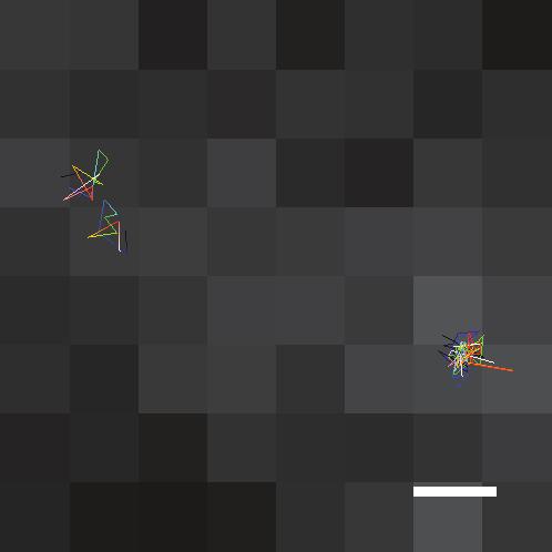
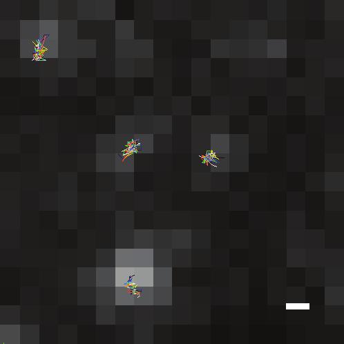
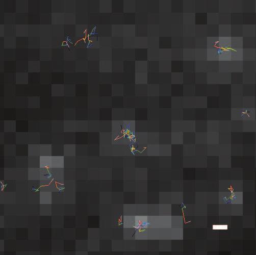
121 Chapter 4: Coupled, circumferential motions of the cell wall synthesis machinery and MreB filaments in B. subtilis 112 Before vancomycin After vancomycin Pbp2A MreD MreC Mbl Figure 4.17: (Continued).

122 Chapter 4: Coupled, circumferential motions of the cell wall synthesis machinery and MreB filaments in B. subtilis 113 Figure 4.18: (A) Kymographs of single particle TIRF movies for GFP-Pbp2A (expressed as a replacement) demonstrating reversals in motion. Particles 1 and 3 in the left panel and particles 1, 3, and 4 in the right panel appear on one side of the cell, travel across the cell width, and disappear at the other side when they leave the illumination plane. However, in both movies the particles indicated as 2R travel across the cell, then reverse their direction. Note the intensity and spot width does not change before and after reversal, indicating it is within the same plane before and after reversal. (B) Kymographs of single particle TIRF movies for GFP-Mbl (expressed as a merodiploid) showing reversals in motion. (C) Kymographs of a single particle TIRF movie for GFP-MreBH (expressed as a replacement) demonstrating a reversal in motion. (D) Kymograph showing a pause in the directed motion of GFP-Mbl (expressed at high levels). Strain BDR2061 was grown in the presence of 10mM xylose, and imaged by TIRF microscopy with streaming 1-second acquisition intervals. The particle indicated at position 2 moves directionally, pauses for 7 seconds, and then resumes directional motion. Maximum Intensity projection (MIP) is shown on the left.

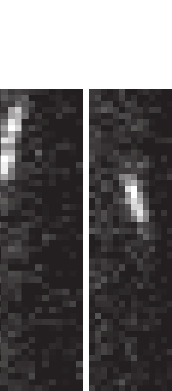
123 Chapter 4: Coupled, circumferential motions of the cell wall synthesis machinery and MreB filaments in B. subtilis 114 A - GFP-Pbp2A Reversals 1 2R µm 0.5 µm 1 2R R nm 800 nm Time (59 sec) Time (47 sec) Cell Maximum Intensity Projection (MIP) reversal Cell MIP reversal B - Mbl Reversals 0.5µm 1R 2 1R Time (59 sec) Time (90 sec) Time (60 sec) µm 0.5 µm Cell MIP reversal Cell MIP reversal Cell MIP reversal C - MreBH Reversal 1 2 3R D - Mbl pause R 0.5 µm Time (73 sec) 0.4um 0.4um Cell MIP pause Time (43 sec) Cell MIP reversal Figure 4.18: (Continued).

124 Chapter 4: Coupled, circumferential motions of the cell wall synthesis machinery and MreB filaments in B. subtilis 115 Figure 4.19: (A) Kymographs of single particle TIRF movies for GFP-Mbl(expressed as merodiploid), showing that proximal foci on one surface of the cell move in opposing directions. Particles appear on one side of the cell, travel across the cell width 3 pixels ( 480 nm), and disappear at the other side (particles 2, 3, and 4) or bleach (particle 1). In this example, particles within short distances (indicated between kymograph bars) move in alternating opposite directions. Under our growth conditions, B. subtilis cells (within chains) are on average 3 µm long. These data demonstrate that Mbl can move in opposite directions on the surface of one bacterium, as at least 2 of these traces must exist in one cell. Note that the GFP-Mbl focus indicated 2 undergoes a blinking event mid-trajectory. Each pixel is 160 nm. (B) Similar to A, showing kymographs of single foci TIRF movie for GFP-Mbl moving in opposing directions. Kymograph 1X displays 2 foci moving in opposing directions within a 1 horizontal pixel range, as manifested by the crossover X in the kymograph. Kymographs 2+3 and 5+6 show 2 particles moving in opposing directions separated by 1 pixel (160 nm). Pixels are 160 nm. (C) Kymograph showing 2 foci of GFP-Pbp2A moving in opposing directions within a 1 horizontal pixel range, as manifested by the crossover X in the kymograph.

125 Chapter 4: Coupled, circumferential motions of the cell wall synthesis machinery and MreB filaments in B. subtilis 116 A C 0.5um nm 800nm 480nm Time (38 sec) Cell MIP 1 pixel crossover Time (19 sec) 4 Cell MIP 1X B 0.5um 1 pixel crossover 160nm 160nm Cell MIP 1X Time (52 sec) Figure 4.19: (Continued).

126 Chapter 4: Coupled, circumferential motions of the cell wall synthesis machinery and MreB filaments in B. subtilis 117 Elongation Figure 4.20: Model for the rotary insertion of new cell wall material in B. subtilis. PG synthetic complexes (blue), which may exist as multiple or single units, and their associated MreB filaments (red) move axially around the cell circumference in both directions, inserting bands of new PG during their transit (green). These complexes can reverse their motion, which may reflect the cessation of one synthetic event and the initiation of a new radial band. Lytic enzymes Synthetic PBP s MreC Precursors RodZ Directed Movement MreD RodA PG Precursor synthesis Figure 4.21: Model for the directed motions of the PG elongation machinery and MreB filaments. PG precursor generating enzymes, bound to MreB, provide a local pool of lipid-linked muropeptide precursors (green arrow) that PBPs incorporate into the newly synthesized glycan strands (green). Their processive insertion drives the movement of the PG elongation machinery along the cell wall, pulling the associated MreB filaments and precursor synthesis complexes.

127 Chapter 5 Conclusions and discussions 5.1 Brief review of this thesis This thesis began with the introduction of super-resolution fluorescence microscopy techniques, in particular, Stochastic Optical Reconstruction microscopy (STORM). Due to the three dimensional nature of biological structures, the capability of imaging cellular structures in 3D with sub-diffraction-limit resolution was much needed. In Chapter 2, we describe the technical extension of STORM to all three dimensions using optical astigmatism, and show 3D STORM images of cellular nanoscopic structures without physically or optically scanning the specimen. Since STORM is inherently light microscopy based and compatible with live-cell imaging applications, STORM can be readily applicable to many arenas of biological systems. Specifically, in Chapter 3, we show the use of 3D STORM in conjunction with biochemical assays to investigate nucleoid associated proteins in live bacteria. We demonstrate that H- 118

128 Chapter 5: Conclusions and discussions 119 NS, a global transcriptional silencer NAP, forms a few compact clusters in the cell for sequestering regulated genes into the clusters and thereby organizing the chromosome in E. coli. In another application of fluorescence detection and localization, in Chapter 4, we describe using the same high-precision fitting method for single particle tracking to study MreB paralogs (actin-like proteins in bacteria) in B. subtilis. Contrary to the previous belief that MreB forms one helix which provides a single scaffold for cell wall elongation, our results show that MreB filaments are discrete, and move independently circumferentially around the cell body, largely driven by the cell wall elongation machineries. Finally, we make brief concluding remarks in this chapter, here and as follows. 5.2 Discussions Less than a decade ago, the limitation on the resolution of fluorescence microscopy was considered a hard limit. In recently years, various fluorescence techniques that break this diffraction limit by an order of magnitude improvement have emerged. STORM (and PALM, FPALM) as one category of these methods, utilizes single molecule localization to accurately find out the positions of all the fluorescent probes within a sample. Image resolution as high as < 10 nm in the lateral dimensions and < 20 nm in the axial direction has been demonstrated with STORM [19,33,63,100, 123]. Advances of STORM including those beyond this thesis have allowed threedimensional imaging of nanoscopic structures [63,100,123] (see also Chapters 2 and 3 of this thesis), imaging multiple cellular components simultaneously [33, 63, 124] (see

129 Chapter 5: Conclusions and discussions 120 also Chapter 3) and capturing molecular dynamics in living cells [124]. The question of how much new information is obtained with STORM, and what studies can benefit from a further improved STORM technique, is closely related to the power and versatility of the technique itself. Despite the interdependence between the technical improvement aspect and the biological applications of STORM, we will discuss these two aspects in the following paragraphs in a semi-independent manner. We first discuss and review general principles and accomplishments, many of which not presented in this work, on improving the technique of STORM. Following that, we show that bacterial cell biology, among many biological research fields, is a particularly interesting subject that will continue to benefit vastly from the applicability of the STORM technique in many years to come. Finally, we conclude the thesis by presenting an example of a contentious research topic bacterial transcripts that STORM will very likely help shed light on in the near future Technical aspects of STORM Spatial resolution The spatial resolution of STORM is not limited to < 10 nm in lateral dimensions and < 20 nm in the axial direction. In fact, the STORM method can provide almost arbitrarily high spatial resolutions. The spatial resolution of STORM imaging depends on the following factors: 1. detection efficiency of the microscope system,

130 Chapter 5: Conclusions and discussions brightness of the fluorophores, 3. residual fluorescence intensity of dark-state fluorophores, 4. the rate of spontaneous activation of the fluorophores, 5. labeling efficiency and density, 6. size of the labels. Firstly, the localization precision of single molecules depends much on the detected photon number (see Section 1.3), so the detection efficiency and the brightness of the fluorophore are important aspects. Secondly, the density of labels is a factor that determines the resolution as well. Suppose in an extreme case where only a tiny fraction of the structure is labeled, even with nanometer precision in localizing the labels, the constructed STORM image with very few localizations still cannot reflect the true structure, due to limited sampling frequency [36,124,125]. A rigorous treatment of this principle is the Nyquist-Shannon sampling theorem [126], which states that the resolution due to finite sampling is Nyquist resolution = 2 d 1/D, where D is the dimensionality (D = 1, 2, 3), and d is the sampling density in D dimensions, i.e., the number of molecules per unit length (D = 1), area (D = 2), or volume (D = 3). Factors 3 6 determine the label density which in turn affects the image resolution. In more detail, factors 3 and 4 limit the maximum labeling density such that molecules will be sparse enough to allow the detection of individual single

131 Chapter 5: Conclusions and discussions 122 molecules above the background. Labeling efficiency, defined as the ratio of labeled targets and all targets, practically determines the labeling density for a given target structure. Finally, the size of the labels affects the resolution in multiple ways: First, with a resolution of a few nanometers demonstrated using a small molecule dye labeling scheme, the distance between the target and the point of emission is no longer negligible. Secondly, the size of the labels also affects labeling efficiency, because biological environments are densely packed, leaving targets more accessible for smaller labels than bigger labels. Temporal resolution Since many biological processes happen at a fast time scale, the temporal resolution (data acquisition speed) of STORM is also an important consideration. Because constructing an image from the accumulation of switching fluorophores coordinates takes time, there is an inherent trade-off between time and spatial resolutions. The following simple example illustrates this trade-off: In order to achieve a Nyquist resolution (see above) of 20 nm for each image, the label density d needs to be 10 4 molecules per µm 2 for each image. Suppose on average 100 molecules are localized in 2D per second per µm 2, it takes 100 seconds to construct one image, and thus the time resolution is 100 seconds; Now assume the same rate of data acquisition but aim for a lower Nyquist resolution of 40 nm for each image, the label density d needs to be only 2500 molecules per µm 2 for each image, so the time resolution becomes 25

132 Chapter 5: Conclusions and discussions 123 seconds in this case. In essence, if given the same data acquisition speed, a higher desired time-resolution effectively translates into lower temporal resolution, and vice versa. Switching the fluorophores faster by using improved photoswitching fluorophores and/or strong laser illumination is a common method to speed up data acquisition, which leads to a higher temporal resolution with the same desired Nyquist resolution. 2D STORM with a high spatiotemporal resolution of 25 nm and 0.5 second has been recently demonstrated [124]. 3D spatial resolution of 30 nm in the lateral direction and 50 nm in the axial direction at time resolutions as fast as 1 2 s with several independent snapshots have been attained with live-cell 3D STORM [124]. In summary, STORM will provide even higher spatiotemporal resolution with the future development of small, bright, fast-switching probes, stable instruments, and high-efficiency data analysis algorithms Applying STORM to bacterial cell biology: Rational and a brief review of previous work Although STORM is still a relatively new invention, the ability of STORM to determine ultrastructural features in cells at physiological conditions at the nanoscopic scale opens a new window for bioimaging, providing important new insights into biological systems by unveiling previously unseen structural information of molecular structures. Since STORM is based on traditional sample preparation and labeling

133 Chapter 5: Conclusions and discussions 124 methods commonly used for fluorescence microscopy, STORM can be readily applied to studies of many biological systems, such as in vitro reconstituted systems, cells, tissues and whole organisms [127]. One particularly interesting territory of applying super-resolution fluorescence microscopy techniques to investigate may be bacterial cell biology. Bacteria cells, despite being widely used model systems for studying molecular biology, were long thought to be bags of randomly distributed enzymes and nucleic acids. It was not until in recent years that scientists view on bacteria has undergone major changes. Microbiologists have started to realize that the bacteria cell contains highly organized chromosomes [67] and other structures, many of which have yet to be studied in detail. In an E. coli cell, proteins, nucleic acids, and small molecules are packed into a small cylindrical volume with 800 nm diameter and 2 5 µm length. Processes which are crucial for the cell s survival and division, such as DNA replication, transcription, translation, occur concurrently in an orchestrated manner. This requires functional regulation and spatial organization. Although there have been substantial studies and findings on the biochemistry, molecular biology, genetics, atomic structure aspects of the biology of E. coli, it remains largely unknown how various cellular components are spatially distributed in an E. coli cell, and how the spatial distribution of cellular components implicates and effects their respective regulatory roles and the overall coordination. As a matter of fact, it is arguably true that our understanding of the localization or motion of proteins and small molecules in prokaryotes lags behind that in eukaryotic cells. This is in part due to the small size of bacteria cells, which is

134 Chapter 5: Conclusions and discussions 125 smaller or comparable to the resolution limit of fluorescence microscopy due to light diffraction, leaving many spatial organizations and sub-cellular structures too small to be resolved. Recent emergence of super-resolution fluorescence microscopy techniques has demonstrated nanometer resolution and great suitability for cell biology research in general, and bacterial cell biology study, in particular, as well. The work presented in this thesis describe application of STORM in studying nucleoid associated proteins in E. coli [128] (Chapter 3) and the application of high-precision single particle tracking in studying cell wall synthesis machinery dynamics in B. subtilis [118] (Chapter 4). Using STORM/(F)PALM, major E. coli chemotaxis proteins (Tar receptor, CheY, and CheW) were found to form clusters whose sizes were roughly exponentially distributed. The location and size distributions were consistent with a stochastic self-assembly model not requiring an active transport mechanism [129]. STORM/(F)PALM was also used to image the C. crescentus chromosome segregation system (the ParABS/Par system), and revealed that the Par system resembled the eukaryotic mitotic spindle in terms of the physical appearance and operating principles [130]. FtsZ protein, the tubulin-like ring-like structure important for bacterial cell division were found to adopt a previously unknown compressed helical confirmation in E. coli [131]. The same proteins in C. crescentus were also examined by 3D STORM/(F)PALM using optical astigmatism [132]. FtsZ in C. crescentus formed an open shape during the stalked stage and a dense focus during the pre-divisional stage. These early works of using STORM/(F)PALM to study microbiology shows great

135 Chapter 5: Conclusions and discussions 126 application potential of the approach Using STORM to study bacterial transcripts: Future work As an example, here we describe a specific microbiology system (bacterial mr- NA) where STORM can be a useful and indispensable imaging tool. An E. coli cell, lacking a nucleus or membrane-bound organelle, does not have clearly divided compartments. The chromosomal DNA along with some abundant DNA binding proteins form a structure called nucleoid (similar to the membrane-bound nucleus in eukaryotic cells) in the middle of the cell, with roughly half the size of the cell. In E. coli, transcription and translation are coupled. One operon (DNA) could be transcribed by multiple RNA polymerase proteins to make multiple transcripts simultaneously depending on promoter strength and other regulatory factors; One mrna, including nascent ones, could be translated by multiple ribosomes (called polysomes or polyribosomes) simultaneously. The coupling happens in the cytoplasm and nucleoid (as there is no clear boundary between the two) of the E. coli cell. mrna, required for both transcription and translation, plays a central role in both processes. More specifically, the localization or motion, degradation, and copy numbers of mrnas have profound implications on transcription and translation, and hence the other crucial life processes. STORM is capable of probing static and time-dependent spatial distributions of multiple components (e.g., transcripts, DNA loci, and proteins,) simultaneously.

136 Chapter 5: Conclusions and discussions 127 STORM assays centered on imaigng bacterial transcripts can potentially uncover previously unseen transcript organizations and mechanisms, and serve as a foundation to build a hollistic view of gene expression machineries in E. coli. In summary, the STORM technique has provided novel insights into biological structures and processes. Considering the rapid development on the technical aspects of STORM and the numerous applications, we expect that the approach will continue to improve to be more versatile and powerful, and that wider and broader applications of the technique will lead to new exciting findings on complex biological structures and dynamics.

137 Appendix A 3D localization precision analysis of single fluorescence emitters Calculating individual fluorophores positions by fitting of the point spread function allows the localization of single molecules to a high precision that is unlimited by light diffraction [22,23]. Localization precision of single fluorescence emitters is a useful parameter in describing the power of imaging systems. The localization precision in the two lateral dimensions has been shown in reference [22]. With the introduction of optical astigmatism into the imaging system as shown in Chapter 2, the localization precision in the axial direction (z) is a new subject of interest. In this chapter, we present an examination on the 3D (x,y and z) localization precision of various position-determination algorithms on an imaging system with optical astigmatism. We first describe the formulation of deriving xy localization errors developed by Bobroff[133]andsubsequently usedbythompsonet al [22]. Weusethesamemethod 128

138 Appendix A: 3D localization precision analysis of single fluorescence emitters 129 to derive the xy localization errors of elliptical images of individual fluorophores in a microscope system with optical astigmatism (Section A.1). Next, in Section A.2, we analyze the precisions for image width measurements, because the widths encode the axial (z) position information. In Section A.3, the results of the width precision analysis are used to derive the localization precisions in z for various z-calculation algorithms, thebest ofwhich is chosen to beour algorithmin3dstorm localization data analysis. Finally, in Section A.4, we conclude by reporting the 3D localization precisions at different heights (z) in an astigmatic imaging system. We also confirm that the calculations of 3D localization precisions shown in this chapter agree very well with Monte Carlo simulations. A.1 Localization precision in lateral dimensions(xy) Single fluorescent particle imaging combined with high-precision centroid-finding algorithms serves as a powerful tool to allow localization of fluorescent objects with a high precision unlimited by the diffraction of light. The intensity profile of a single fluorescence emitter on the detector (e.g., a charge coupled device camera) is called the point spread function (PSF). This profile is theoretically a pixelated Airy function, but in practice is often approximated by a pixelated two-dimensional Gaussian g(x,y;x 0,y 0,s x,s y,n) on top of the background: G(x,y;x 0,y 0,s x,s y,n,b;a) = g(x,y;x 0,y 0,s x,s y,n)+b 2 /a 2, (A.1) (x x 0 ) 2 N (y y 0) 2 e 2s 2 x 2s 2 y +b 2 /a 2, 2πs x s y

139 Appendix A: 3D localization precision analysis of single fluorescence emitters 130 where N is the number of detected photons in the spot, (x 0,y 0 ) is the centroid of the PSF, b 2 is the average background in number of photons per pixel, a is the pixel size of the detector, (so b 2 /a 2 is the average background per unit detector area), and s x and s y are standard deviations of the Gaussian in x and y, respectively. Note that s x and s y are in general different if the imaging system has optical astigmatism (see Chapter 2). A.1.1 General derivation Given S(x,y) is the measured photon counts in pixel (x,y), in a least squares fit to obtain parameters x 0,y 0,s x,s y,n and b, the sum of squared errors, χ 2 (x 0,y 0,s x,s y,n,b;a) = x,y (G(x,y;x 0,y 0,s x,s y,n,b;a) S(x,y)) 2 σ 2 (x,y;x 0,y 0,s x,s y,n,b;a) (A.2) is minimized, where σ 2 is the expected (according to fit G(x,y;x 0,y 0,s x,s y,n,b;a)) variance in the photon count in pixel (x,y). σ 2 is the sum of emitter photon shot noise g and the per-pixel background b 2 /a 2 : σ 2 (x,y;x 0,y 0,s x,s y,n,b;a) = g(x,y;x 0,y 0,s x,s y,n)+b 2 /a 2. (A.3) The criterion of minimizing χ 2 gives x 0 χ 2 (x 0,y 0,s x,s y,n,b;a) = 0. (A.4) For notional simplicity, we omit the arguments s x,s y,n,b and a in functions G, g, χ 2 and σ 2 in many places. Inserting Equation A.2 into A.4 gives x 0 χ 2 (x 0,y 0 ) = x,y x 0 (G(x,y;x 0,y 0 ) S(x,y)) 2 σ 2 (x,y;x 0,y 0 ) = 0, (A.5)

140 Appendix A: 3D localization precision analysis of single fluorescence emitters 131 which is equivalent to x,y Similarly, x,y G(x,y;x 0,y 0 ) S(x,y) σ 2 (x,y;x 0,y 0 ) y 0 χ 2 (x 0,y 0 ) = 0 leads to G(x,y;x 0,y 0 ) S(x,y) σ 2 (x,y;x 0,y 0 ) G(x,y;x 0,y 0 ) x 0 G(x,y;x 0,y 0 ) y 0 ( ( 1 G(x,y;x 0,y 0 ) S(x,y) 2σ 2 (x,y;x 0,y 0 ) 1 G(x,y;x 0,y 0 ) S(x,y) 2σ 2 (x,y;x 0,y 0 ) ) ) = 0. (A.6) = 0. (A.7) We denote the solution 1 of (x 0,y 0 ) in Equations A.6 and A.7 as (x 00,y 00 ). Expanding G(x,y;x 0,y 0 ) around (x,y;x 00,y 0 ) gives which further leads to G(x,y;x 0,y 0 ) G(x,y;x 00,y 0 )+(x 0 x 00 ) G(x,y;x 00,y 0 ) x 0, (A.8) G(x,y;x 0,y 0 ) S(x,y) = G+g x0 x, (A.9) where G G(x,y;x 00,y 0 ) S(x,y) is roughly the error in counted photons in pixel (x,y), 1 Actually, it is the equation set of x 0 χ 2 (x 0,y 0,s x,s y,n,b;a) = y 0 χ 2 (x 0,y 0,s x,s y,n,b;a) = 0 χ 2 (x 0,y 0,s x,s y,n,b;a) = χ 2 (x 0,y 0,s x,s y,n,b;a) = 0 s x s y N χ2 (x 0,y 0,s x,s y,n,b;a) = 0 b χ2 (x 0,y 0,s x,s y,n,b;a) = 0 that determines the solution of (x 0,y 0,s x,s y,n,b).

141 Appendix A: 3D localization precision analysis of single fluorescence emitters 132 g x0 G x 0 g x 0 evaluated at (x,y;x 00,y 0 ), and x x 0 x 00 is the error in x. Assuming g(x,y;x 0,y 0 ) x 0 g(x,y;x 00,y 0 ) x 0 g x0 and ( x) 2 = 0, Equation A.6 becomes Rearranging the terms gives ( G+g x0 x g x,y σ 2 x0 1 G+g ) x 0 x 0. 2σ 2 (A.10) x,y Gg x0 σ 2 ( 1 G 2σ 2 ) + x x,y g 2 x 0 σ 2 ( 1 G ) 0. σ 2 (A.11) Thus, we have the following expression of the error in determining x x x,y Gg x0 σ 2 ( x,y g 2 x 0 σ 2 ( 1 G ) 2σ 2 1 G ). (A.12) σ 2 Assuming the errors in counting photons are relatively small ( G σ 2 = g + b 2 ) ( ) Gg x0 2 Gg x0 x,y σ 2 gives x gx 2, which gives ( x)2 x,y σ 2 ( 0 g 2 ) 2. Averaging over G x 0 x,y σ 2 x,y σ 2 gives the expectation value of ( x) 2 : ( x) 2 = = ( ) 2 Gg x0 x,y σ 2 ( gx 2 ) 2 0 x,y σ 2 ( ) 2 /( Gg x0 ( / )) 2 g 2 x,y σ 2 x0 σ 2 x,y ( )( G(x i,y j ;x 00,y 0 )g x0 (x i,y j ;x 00,y 0 ) ) G(x k,y l ;x 00,y 0 )g x0 (x k,y l ;x 00,y 0 ) x i,y j σ 2 x k,y l σ ( 2 ( / )) 2 g 2 x0 σ 2 x,y

142 Appendix A: 3D localization precision analysis of single fluorescence emitters 133 G(x i,y j ;x 00,y 0 ) G(x k,y l ;x 00,y 0 ) g x0 (x i,y j ;x 00,y 0 )g x0 (x k,y l ;x 00,y 0 ) x i,y j,x k,y l σ 2 (x i,y j ;x 00,y 0 )σ 2 (x k,y l ;x 00,y 0 ) = ( ( / )) 2. g 2 x0 σ 2 x,y Because the errors of photon counts in different pixels are independent, we have G(x i,y j ;x 00,y 0 ) G(x k,y l ;x 00,y 0 ) = δ i,k δ j,l G 2 (x i,y j ;x 00,y 0 ) = δ i,k δ j,l σ 2 (x i,y j ;x 00,y 0 ), (A.13) where δ is the Dirac delta function. Inserting the above equation to the expression of ( x) 2 gives ( ) g 2 x 0 ( x) 2 x,y σ 2 ( ) 2 = x,y g 2 x 0 σ 2 1 x,y g 2 x 0 σ 2 = x,y 1 g 2 x 0 g +b 2 /a 2. (A.14) In summary, we have so far derived the expression of the variance of x or y using least-squares fitting assuming a Gaussian PSF (Equation A.1): Var(x) = x,y 1 g 2 x 0 g +b 2 /a 2, Var(y) = x,y 1 g 2 y 0 g +b 2 /a 2. (A.15) To calculate the lateral localization precisions, one can numerically integrate the above equations or use approximate analytical formulae derived later in this chapter. Next, we simplify Equations A.15 in two extreme cases: the photon-shot noise limited case where the noise mainly comes from the Poisson shot noise of the fluorescence emitter, and the background noise limited case where the noise mainly comes from sources other than the individual fluorescence emitter (e.g., autofluorescence of

143 Appendix A: 3D localization precision analysis of single fluorescence emitters 134 the coverglass). The first case is also called the low background or high photon count case since the background level b 2 is negligible. Conversely, the latter case is also called the high background or low photon count case. A.1.2 Low background limit In a low background case, the background level b 2 is much lower than the photon count of the fluorescence emitter, i.e., b 2 N, so Equation A.15 becomes Var(x) 1 gx 2 0 /g. x,y (A.16) (x x 0 ) 2 Plugging in G(x,y;x 0,y 0 ) = N (x x (y y 0) 2 0) x 0 2πs 3 x s e 2s 2 x 2s 2 y y gives gx 2 0 /g x,y N 2πs 5 x s y (x x 00) 2 (y y 00) 2 (x x 00 ) 2 e 2s 2 x 2s 2 y dxdy = N/s 2 x. (A.17) Considering the noise due to pixelation on the pixelated detector, we have Var(x) s2 x +a 2 /12 N, when the background is low, i.e., b 2 N (A.18) We note that this result is the same as the central limit theorem predicts 2. 2 The scaling relation is natural in that it is the central limit theorem applied to the mean of N independent and identically distributed (i.i.d.) random variables Gaussian-distributed (x, y) coordinates in this case. A large background would have made these variables not i.i.d. However this current case has a negligible background.

144 Appendix A: 3D localization precision analysis of single fluorescence emitters 135 A.1.3 High background limit In an extreme case where the background is much brighter than the fluorescence emitter, i.e., N b 2, Equation A.15 becomes Var(x) b 2 /a 2/ gx 2 0. x,y (A.19) Approximating the sum with a double integral gives: ( ) 2 g(x,y;x00,y 0 ) x,y x 0 = N 2 (x x 00) 2 (y y 00) 2 (2πs 3 x s y) 2 (x x 00 ) 2 e s 2 x s 2 y dxdy N 2 8πs 3 xs y. (A.20) So when the background is much higher than the emitter fluorescence (b 2 N), the variance of x can be expressed as Var(x) 8πs3 xs y b 2 a 2 N 2. (A.21) A.1.4 Summary The noise contributions from the emitter fluorescence and the background are more or less independent of each other, thus we can combine the two variance terms in Equations A.18 and A.21: Var(x) s2 x +a2 /12 N Var(y) s2 y +a2 /12 N + 8πs3 x s yb 2 a 2 N 2, (A.22) + 8πs3 y s xb 2 a 2 N 2. (A.23) Alternatively, numerically integrating Equations A.15 can provide more accurate estimations of Var(x) and Var(y) than the formulae above especially when the background is comparable with the individual emitter s photon number N.

145 Appendix A: 3D localization precision analysis of single fluorescence emitters 136 In summary, we have derived the xy localization precisions in an imaging system with optical astigmatism. A.2 Uncertainty of the image widths In the 3D STORM localization data analysis, the z information is encoded in the widths of the elliptical spots. Calculating the localization precision in z requires knowing the precisions of the width measurements, which we study in this Section. The approach we take to derive the precisions of widths is similar to that in the previous section. A.2.1 General derivation Similar to Equation A.4, minimizing χ 2 also means s x χ 2 (x 0,y 0,s x,s y,n,b;a) = 0. (A.24) Using similar derivations that lead to Equations A.15, the variances of s x and s y can be shown to be Var(s x ) 1 / x,y ( g ) 2 s x g +b 2 /a, Var(s y) 1 / ( g ) 2 s y 2 g +b 2 /a. 2 x,y (A.25) Similar to the previous section, we derive the exact analytical form of the above equations in two extreme cases: low background and high background cases.

146 Appendix A: 3D localization precision analysis of single fluorescence emitters 137 A.2.2 Low background limit When the background is much lower than the photon number from the emitter, i.e., b 2 N, the variance of s x can be approximated as / ( ) 2 Var(s x ) 1 g / g = s 2 s x/(2n). x x,y (A.26) Alternatively, random variable (N 1)s2 x s 2 x is distributed according to the chisquare distribution with N 1 degrees of freedom. According to the properties of the chi-square distribution 3, we have (N 1) 2 Var(s 2 x ) = 2(N 1) s2 x, s 2 x 2 s 2 x which leads to Var(s 2 x ) = 2 s2 x 2 /(N 1), giving Var(s x ) = Var(s2 x ) 4 s 2 x = s 2 x /(2(N 1)) s 2 x /(2N). (A.27) We note the agreement between Equations A.26 and A.27. Finally, including the pixelation variance a 2 /12 into s 2 x gives Var(s x ) s2 x +a2 /12 2N. (A.28) A.2.3 High background limit When the background is much higher than the photons from the emitter, i.e., b 2 N, the variance of s x is approximately ( g ) 2. (A.29) Var(s x ) b 2 /a 2 / x,y s x 3 The variance is two times the mean of a chi-square distribution.

147 Appendix A: 3D localization precision analysis of single fluorescence emitters 138 ( ) 2 g Plugging in dxdy = 3N2 s x 16πs 3 gives xs y Var(s x ) 16πs3 xs y b 2 3a 2 N 2 (A.30) A.2.4 Summary Similar as in the previous section, assuming independence between the contributions from the emitter photon noise and the background noise, and combining various terms at the two extremes give Var(s x ) s2 x +a2 /12 2N Var(s y ) s2 y +a 2 /12 2N + 16πs3 x s yb 2 3a 2 N πs3 ys x b 2 3a 2 N 2 (A.31) (A.32) Alternatively, numerically integrating the following formulae can provide more accurate variances of s x and s y : / Var(s x ) 1 x,y ( g ) 2 / s x g +b 2 /a, Var(s y) 1 2 x,y ( g s y ) 2 g +b 2 /a 2. (A.33) A.3 Localization precision in the axial direction (z) With the precisions of the width measurements determined (see Section A.2), we proceed to calculate the precision in z localization for various z-determination algorithms using standard error propagation theory.

148 Appendix A: 3D localization precision analysis of single fluorescence emitters 139 With optical astigmatism, the PSF widths follows these empirical defocusing curves as described briefly in Section 2.4: w x (z) = w x0 1+( z +c x d x ) 2 +A x ( z +c x d x ) 3 +B x ( z +c x d x ) 4, w y (z) = w y0 1+( z c y ) d 2 +A y ( z c y ) x d 3 +B y ( z c y ) y d 4, y where w x0 w y0 is the image width in x or y for a molecule at the focal plane, c x or c y is the offset of the x or y focal plane from the average focal plane (the average focal plane being the z positionwhere the imageis spherical andsymmetrical inbothxand y directions, defined as z = 0), d x or d y is the focal depth of the imaging system, and A x, B x or A y, B y are coefficients of higher order terms accounting for the non-ideality of the imaging optics (ideal defocusing curves would have A and B = 0). These parameters for x and y are only slightly different due to approximate symmetry between x and y. For simplicity, we assume A x = A y = 0,B x = B y = 0,w x0 = w y0,c x = c y = c, and d x = d y = d in this section. Let s x w x /2 and s y w y /2 be the standard deviations (half-widths) of the fluorescent molecules in x and y, respectively. The defocusing curves then become s x (z) = s 0 1+( z +c d )2, s y (z) = s 0 1+( z c d )2. (A.34) A.3.1 Methods for calculating z positions Forany measured pairof s x ands y, therearemultiple methods ofcalculating z. In Section 2.4 we described the method that we employ. In this section, we demonstrate that the method we use provides the lowest error among several common method

149 Appendix A: 3D localization precision analysis of single fluorescence emitters 140 candidates used previously in the literature. Methods 1, 2 and 3 are direct manipulations of Equations A.34. Using Method 1, z is directly calculated from the difference of the squared standard deviations in x and y: z 1 (s x,s y ) = d2 (s 2 4cs 2 x s 2 y). (A.35) 0 Method 2 uses the sum of the squared standard deviations in x and y to calculate z: z 2 (s x,s y ) = sign(s x s y ) ( s 2 x +s 2 ) y 1 c 2. Method 3 [58] uses the larger of s x and s y to determine the z: 2s 2 0 (A.36) ) 2 ( max(sx,s y ) z 3 (s x,s y ) = sign(s x s y ) d 1 c (A.37) s 0 s 2 d x 1 c (if s s 2 x > s y ) 0. (A.38) c d s2 y 1 (if s s 2 x s y ) 0 Finally, Method 4, as described in Section 2.4 is our method of choice. Briefly, the z position of a molecule can be derived by searching the z-calibration curve (i.e., widths w x,calib, w y,calib versus z curve, Fig. 2.1B) to find a best match. A best match is defined as when the expression (w 1/k x w 1/k x,calib )2 +(w 1/k y w 1/k y,calib )2 (k 1) is minimized.

150 Appendix A: 3D localization precision analysis of single fluorescence emitters 141 A.3.2 z localization precisions for the methods and 3: It is straightforward to calculate the variances of z determined by Methods 1, 2 Var(z 1 ) = d4 ( s 2 4c 2 s 4 x Var(s x )+s 2 y Var(s y) ), (A.39) 0 d 4 ( Var(z 2 ) = ) s 2 2s0( 2 d 2 (s 2 x +s2 y 2s2 0 ) 2c2 s 2 x Var(s x )+s 2 y Var(s y) ), (A.40) 0 Var(z 3 ) = d 2 s 2 0( (max(sx,s y )) 2 s 2 0 ) (max(s x,s y )) 2 Var(max(s x,s y )), (A.41) where Var(s x ) and Var(s y ) can be computed using formulae in Subsection A.2.4. The variance of z determined by Method 4 is derived as follows. An ideal pair (s x,s y ) satisfy the defocusing curves (Equations A.34) perfectly. However, the measured standard deviations have some small errors ds x and ds y. Because the errors of s x ands y areindependent, wecanseparate thenoisecontributions ofds x andds y. We denote the measured standard deviations as (s x +ds x,s y +ds y ), and let ds y = 0 first, in order to study the propagation of uncertainty of ds x to the calculated z position. Suppose we have an ideal pair (s x,s y ) that satisfy Equations A.34 perfectly. We schematically represent theideal defocusing curve inthes 1/k x s1/k y (k 1)spaceusing a straight line near the given (s 1/k x,s 1/k y ) (point A in Fig. A.1). If the measurement of s x has an error of ds x, the measured point in the s 1/k x s 1/k y A.1, (s 1/k x +ds 1/k x,s1/k y ), space is point B in Fig. whereds 1/k x sx 1/k 1 ds x /k istheerrorofs 1/k x. Next, wesearchonthedefocusingcurve (line AC) in the s 1/k x s 1/k y space to minimize the distance from the measured point

151 Appendix A: 3D localization precision analysis of single fluorescence emitters 142 s 1/k y s 1/k x C (s1/k x +cos 2 θds 1/k x,s1/k y +cosθsinθds 1/k x ) A θ B (s 1/k x,s1/k y ) (s 1/k x +ds 1/k x,s1/k y ) Figure A.1: The defocusing curve is shown as a line AC in the s 1/k x s 1/k y space. Due to measurement uncertainty in the s x, point A is measured to be point B, which is then matched to point C on the defocusing curve. Point C is the closet point on the defocusing curve to point B in the s 1/k x s 1/k y space, according the Method 4. B to the match (denoted as C) on the curve. Geometrically, line BC is perpendicular to line AC. Thus, C has a coordinate of (s 1/k x +cos 2 θds 1/k x,s 1/k y +cosθsinθds 1/k x ) in the s 1/k x s 1/k y space, where θ is the angle of the s 1/k x s 1/k y AC) with respect to the positive s 1/k x axis, and its tangent tanθ = The found match (point C) in the s x s y space is 4 defocusing curve (line ( ) s 1/k y. s 1/k x z (s x +cos 2 θds x,s y +cosθsinθ ( sy s x ) 1 1/kdsx ). 4 This is because (s 1/k x +cos 2 θds 1/k x )k s x +ksx 1 1/k cos 2 θsx 1/k 1 ds x /k = s x +cos 2 θds x and (s 1/k y +cosθsinθds 1/k x )k s y +cosθsinθ ( sy s x ) 1 1/k ds x

152 Appendix A: 3D localization precision analysis of single fluorescence emitters 143 We denote the z position corresponding to (s x,s y ) according to Equations A.34 as z 0, and we prove 5 that point C also satisfies Equations A.34 with a different z: z = z 0 +cos 2 θ z s x ds x z 0 +cosθsinθ ( sy s x ) 1 1/k z s y ds x, where z d = ± s x s 2 x s s x s 2 0 can be directly derived from Equations A.34., z d = ± s y s 2 y 1 s 2 0 s y s 2 0 (A.42) Let dz = z z 0 being the error of z due to the uncertainty of measuring s x alone, and we have dz = cos 2 θ z s x ds x. So the variance of z calculated using Method 4 due to the uncertainty of s x alone is ( ) 2 z Var(z 4 ) = cos 4 θ Var(s x ) (A.43) s x ( ) 2 z We will now express Var(z 4 ) using s x and s y by explicitly calculating cos 4 θ. s x Plugging in the following equations cos 2 θ = 1/(1+tan 2 θ) tanθ = c z c+z 5 The equation cos 2 θ z s x ds x cosθsinθ ( sy s x ( ) sy 1/k 2 s x ) 1 1/k z s y ds x can be proven by using ( ) s 1/k y tanθ = s 1/k x z = s 1/k y z s 1/k x z = ( sy s x ) 1/k 1 s y z s x z = ( sy s x ) z 1/k 1 s x. z s y

153 Appendix A: 3D localization precision analysis of single fluorescence emitters 144 tan 2 θ = s2 y s2 0 s 2 x s 2 0 ( ) 2 z d 2 s 2 x = ( ) sy 2/k 4 s x s x (s 2 x s 2 0)s 2 0 gives Similarly, ( ) 2 z cos 4 θ = ( s x 1+ s2 y s 2 0 s 2 x s2 0 ( sy s x d 2 s 2 x ) ) 2/k 4 2. (s 2 x s 2 0)s 2 0 ( ) 2 z sin 4 d 2 s 2 y θ = s y 1+ s2 x s 2 ( ) 2/k sx (s s 2 y s2 0 s 2 y s2 0)s 2 0 y Finally, considering the uncertainties in both s x and s y and the total variance ( ) 2 ( ) 2 z z Var(z 4 ) = cos 4 θ Var(s x )+sin 4 θ Var(s y ), s x s y we have the following expression for the variance of z for Method 4: Var(z 4 ) = ( 1+ s2 y s2 0 s 2 x s s2 x s2 0 s 2 y s2 0 d 2 s 2 xvar(s x ) ( sy s x ) 2/k 4 ) 2 (s 2 x s2 0)s 2 0 d 2 s 2 y Var(s y) ) 2/k 4 ( sx s y 2 (s 2 y s 2 0)s (A.44) We have reported in Equations A.39, A.40, A.41 and A.44 the expressions of the variances of z obtained by Methods 1 4, respectively. Next, we calculate and plot all these z uncertainty values in a practical situation where the parameters (calibration parameters c, d and s 0, and other parameters N, a, and b 2 ) are similar as in a 3D STORM calibration and imaging experiment [100]:

154 Appendix A: 3D localization precision analysis of single fluorescence emitters s 0 = 160 nm, is the standard deviation of the fluorescence peak w/o astigmatism, 2. c = 200 nm, is the offset of the x or y focal plane from the average focal plane, 3. d = 360 nm, is the focal depth of the microscope, (The ideal defocusing curves according to Equations A.34 are shown in Fig. A.2.) 4. a = 167 nm, is the pixel size, 5. N = 6000, is the detected photon number, 6. b 2 = 36, is the background photon per pixel. Figure A.2: Ideal defocusing curves according to Equations A.34 with s 0 = 160 nm, c = 200 nm, and d = 360 nm. Shown are w x 2s x,w y 2s y.

155 Appendix A: 3D localization precision analysis of single fluorescence emitters 146 We then calculate the z localization precisions for Methods 1 4 (with k = 1,2 or 3) as a function of z in the above configuration by plugging in the values above into EquationsA.33,A.34,A.39,A.40, A.41andA.44(withk = 1,2or3) 6. Noticethatthe z s are random variables distributed according to Gaussian distributions, so the fullwidth-at-half-maximum width (FWHM) is also a measure of the precision. FWHM is directly proportional with the standard deviation, FWHM(z)=2 2log(2) Var(z) Var(z). We plot the FWHM values for z between 0 and 500 nm obtained by Methods 1 4 in Fig. A.3. FWHM(z 1 ) 40 FWHM(z 2 ) FWHM(z 3 ) FWHM(z 4 ) (k=1) FWHM(z 4 ) (k=2) FWHM(z 4 ) (k=3) z (nm) Figure A.3: Theoretical z precisions (FWHM, nm) for z between 0 and 500 nm, for Method 1 (solid red circles), Method 2 (solid blue triangles), Method 3 (solid green squares), Method 4 with k = 1 (open magenta circles), Method 4 with k = 2 (open cyan triangles), and Method 4 with k = 3 (open brown squares). 6 Numerical integrations are carried out using the Mathcad software, PTC.

156 Appendix A: 3D localization precision analysis of single fluorescence emitters 147 It is apparent from Fig. A.3 that Methods 1 3 have consistently larger errors than Methods 4 (compare solid symbols and open symbols). Method 4 with k = 2 is appreciably more accurate than Method 4 with k = 1, but not much more error-prone than Method 4 with k = 3. Thus, Method 4 with k = 2 is our method of choice to determine z in 3D STORM (see Section 2.4 and reference [100]). A.4 3D localization precisions: theory vs simulation In previous parts of this chapter, we have theoretically derived expressions of variances of x, y and z as a function of z. In this section, we compare the theoretical prediction of precisions with precisions obtained from analyzing computer-generated images, and confirm that our derivations agree with the analysis of Monte Carlo simulated data very well. Fig. A.4 shows artificially generated images of a point emitter with increasing z heights. First, for a given z, the widths of the PSF in x and y is calculated according to Equations A.34 using a half width of s 0 = 160 nm, a focal-plane-offset of c = 200 nm, and a focal depth of d = 360 nm. Secondly, the average image at a given z is computed according to Equation A.1 with N = 6000, b 2 = 36, and a = 167 nm. Finally, the photon count in each pixel is generated randomly so that it is Poissondistributed with the expectation being the photon count from the average image. For each z = 0,100,200,300,400, or 500 nm, we use the computer to generate

157 Appendix A: 3D localization precision analysis of single fluorescence emitters 148 z=0 z=100 nm z=200 nm z=300 nm z=400 nm z=500 nm Figure A.4: Artificially generated images of a point emitter at different heights (two images per height are shown). Equations A.34 and A.1, and the following parameters are used in simulating these images: s 0 = 160 nm, c = 200 nm, d = 360 nm, N = 6000, b 2 = 36, and a = 167 nm. All the parameters describing the emitter and the microscope are the same as in the previous section images, and show two of them as examples in Fig. A.4. For each simulated image, we then use least-squares fitting to determine its (x,y) position and widths w x and w y, which are then used to determine its z position using Method 4 (see previous sections) assuming the same ideal defocusing curves we use to generate the images at different heights.