An Irrigated Area Map of the World (1999) Derived from Remote Sensing

Transcription

1 RESEARCH REPORT 105 An Irrigated Area Map of the World (1999) Derived from Remote Sensing Thenkabail, P.S., Biradar, C.M., Turral, H., Noojipady, P., Li, Y.J., Vithanage, J., Dheeravath, V., Velpuri, M., Schull, M., Cai, X. L., Dutta, R. International Water Management Institute IWMI is a Future Harvest Center supported by the CGIAR

2 Research Reports IWMI s mission is to improve water and land resources management for food, livelihoods and nature. In serving this mission, IWMI concentrates on the integration of policies, technologies and management systems to achieve workable solutions to real problems practical, relevant results in the field of irrigation and water and land resources. The publications in this series cover a wide range of subjects from computer modeling to experience with water user associations and vary in content from directly applicable research to more basic studies, on which applied work ultimately depends. Some research reports are narrowly focused, analytical and detailed empirical studies; others are wide-ranging and synthetic overviews of generic problems. Although most of the reports are published by IWMI staff and their collaborators, we welcome contributions from others. Each report is reviewed internally by IWMI s own staff and Fellows, and by external reviewers. The reports are published and distributed both in hard copy and electronically ( and where possible all data and analyses will be available as separate downloadable files. Reports may be copied freely and cited with due acknowledgment.

3 Research Report 105 An Irrigated Area Map of the World (1999) Derived from Remote Sensing Thenkabail, P. S., Biradar, C. M., Turral, H., Noojipady, P., Li, Y. J., Vithanage, J., Dheeravath, V., Velpuri, M., Schull, M., Cai, X. L., Dutta, R. International Water Management Institute P O Box 2075, Colombo, Sri Lanka i

4 IWMI receives its principal funding from 58 governments, private foundations, and international and regional organizations known as the Consultative Group on International Agricultural Research (CGIAR). Support is also given by the Governments of Ghana, Pakistan, South Africa, Sri Lanka and Thailand. Authors: Prasad S. Thenkabail is a Principal Researcher and Head, Global Research Division; Chandrashekhar M. Biradar is a PostDoc scientist; Hugh Turral is a Principal Researcher and Theme Leader; Praveen Noojipady, Yuanjie Li, Jagath Vithanage, Venkateswarlu Dheeravath and Manohar Velpuri are Research Officers; Cai Xueliang and Rishiraj Dutta are Consultants from Partner Institutes in China and India, respectively. All authors, except Schull who is from the Boston University, USA, are attached to the International Water Management Institute A Global Irrigated Area Mapping (GIAM) project of this magnitude and complexity can never be done without substantial and persistent support from many places. We are very grateful to Prof. Frank Rijsberman, Director General of IWMI, for his vision, guidance and financial support; Dr. David Molden, Principal Researcher at IWMI, was instrumental in initial funding and guiding GIAM through the Comprehensive Assessment (CA). Dr. Sarath Abayawardana, former Global Research Director (GRD), was instrumental in laying a strong foundation for the RS\GIS laboratory at IWMI and Julie Van der Bliek, the present GRD head, has continued this support and has steered us towards a spatial data policy at IWMI. All researchers and analysts in the RS\GIS unit have helped in one way or another; we thank Aminul Islam for compiling the excellent groundtruth data of the world and the rainfall data; Wasantha Kulawardana for support when needed; Sarath Gunasinge, and Alankara Ranjith are always there with quiet but strong support in producing maps and flow charts. Jacintha Navaratne provided outstanding secretarial services, most cheerfully. IWMI India office was especially helpful. Thanks to Trent Biggs, Muralikrishna and Parthasarathi. We would like to thank the Food and Agriculture Organization (FAO)/University of Frankfurt (UF) for lively discussions on the two Global Irrigated Area Maps (FAO/UF and IWMI). Specifically, we would like to thank Stefan Siebert and Jippe Hoogeveen. The NASA Goddard Space Flight Center (GSFC) made available the AVHRR time series used in this work. Special thanks to Dr. Ron Smith and his group. The Landsat data were downloaded from the University of Maryland s Global Land Cover Facility (GLCF). Several data sets such as the GTOPO30 1-km and SRTM 90 meter elevation data were downloaded from the USGS\EROS. The forest cover data were sourced from Dr. Ruth DeFries of the University of Maryland. Rainfall data were provided by Dr. Tim Mitchell of East Anglica Climate Research Group and the JERS SAR data from Saatchi and the group. The volunteer groundtruth data from degree confluence project were invaluable. The Google Earth data are state of the art and were widely used. Without these great data sets, made available free of charge, the project would not have been completed. So we are very grateful to these agencies and the numerous people behind them. Thenkabail, P. S.; Biradar, C. M.; Turral, H.; Noojipady, P.; Li, Y. J.; Vithanage, J.; Dheeravath, V.; Velpuri, M.; Schull, M.; Cai, X. L.; Dutta, R An irrigated area map of the world (1999) derived from remote sensing. Research Report 105. Colombo, Sri Lanka: International Water Management Institute. /remote sensing / mapping / irrigated sites / estimation / GIS / assessment/ ISBN ISBN Copyright 2006, by IWMI. All rights reserved. Please send inquiries and comments to: iwmi@cgiar.org

5 Contents 1 Summary ix 2 Introduction 1 3 Background and rationale Irrigation development and trends Estimates of irrigated area 3 4. Data used in creating IWMI s global irrigated area map Primary remote sensing data sets and masks AVHRR data characteristics SPOT data characteristics Mask data GTOPO 30 1-km DEM CRU precipitation and temperature data Forest cover data Secondary data sets JERS-1 SAR derived forest cover ESRI Landsat 150-m GeoCover Google Earth data set Groundtruth data Groundtruth at IWMI: Data collected in field campaigns Public domain groundtruth the Degree Confluence Project Other data sets for comparison purposes 10 5 Methods Image segmentation 11 iii iii

6 5.1.1 Mega-file of segments Classification Class identification and naming process Spectral matching techniques Qualitativespectral matching Quantitative spectral matching Google Earth as a resource for class naming Advanced techniques for class identification Class-naming convention 18 6 Estimating irrigated areas using three methods Irrigated area fraction (IAF) based on Google Earth estimates SPA of pixels based on high-resolution imagery Classification approach Regression relationships Irrigated area fraction coefficient Sub-pixel decomposition technique 24 7 Accuracy assessment Groundtruth data sets from the Global Irrigated Area Mapping Project Other goundtruth Google Earth estimates 26 8 Results Global irrigated area map version 2.0 (GIAM10 km V2.0) Areas of irrigation derived from GIAM10 km map V Irrigated areas of continents, countries and river basins Accuracy assessment of the GIAM10 km map V2.0 and its comparison Accuracies and errors of GIAM10 km map V2.0 using groundtruth Accuracies and errors using Google Earth groundtruth (GEGT) data for the world Accuracies and errors for India in GIAM10 km V Accuracy assessment discussions Accuracies and areas 40 iv iv

7 9. A discussion on mapping irrigated areas and comparison of maps Major irrigation Informal irrigation Comparing global products in India Irrigated area class names GIAM10 km V2.0 products and dissemination Conclusions Annexes Acronyms and abbreviations Literature Cited 62 v v

8 Figures vi Figure 1. Processing chain for the global irrigated area map (GIAM). 6 Figure 2. Mega-file used in GIAM. The mega-file of 159 layers of data which consist of 144 AVHRR 10-km monthly layers from 3 years, 12 SPOT monthly layers from year 1999, single layer of DEM, mean annual rainfall for 40 years, and forest cover. 6 Figure 3. Primary and secondary data sets used in the mega-file. 7 Figure 4a. Summary of analysis to determine irrigation land use classes (part 1). 12 Figure 4b. Summary of analysis to determine irrigation land use classes (part 2). 13 Figure 5. Precipitation less than 360 mm segment (PLT360-segment). These arid or semiarid areas provide distinct contrasts between areas with and without vegetation. 14 Figure 6a. Time-series AVHRR 10-km profile of spectral classes is illustrated for the AOAW-segment. Initially, the AOAW-segment had 350 classes. The plot of some of these classes highlights the spectral characteristics of each class. A quantitative approach to determine which of these classes match is performed through SCS R 2 (e.g., table 4). 15 Figure 6b. Identifying similar irrigated classes using spectral matching. Spectral matching in combination with ground truthing and ideal spectra helps group similar irrigated (shown in dark green, for classes 25, 26, and 27). The same logic was used to group: forests (sown in light green; class numbers 1, 2, 3, 4 and 5), Savanna/Croplands mix (Orange; class 50, 59, 60, 67, 74), and Barren/Deserts (shown in blue; classes 10 to 15). 16 Figure 7. The process of combining classes in spectral matching techniques (SMTs) is illustrated. First, the SCS R 2 -values are determined for a matrix of classes. The time-series spectra of classes with high SCS R 2 - values are then matched. Grouped classes are investigated further, using all other types of information including groundtruth. This leads to distinct groups such as boreal forests and tropical forests. Finally, the classes of similar types are color-coded. 16 Figure 8. Google Earth zoom in views to identify a class. One preliminary class is spread out across the world. The class was investigated using 50 Google sample points that were randomly chosen. The figure shows the spread of the class across the world and Google Earth hi-res image at two locations: Center pivot groundwater irrigation in the USA and surface irrigation in Sudan. 17 Figure 9. Class naming convention. The standardized class naming convention is depicted in this figure. At different levels, the class naming may or may not include a particular category such as scale of irrigation or the intensity. 19 Figure 10. Summary of area abstraction from the 28 irrigation class map. 20 Figure 11. Irrigated area by Google Earth estimate (GEE). For each GIAM10 km-28 classes GEE of irrigated area fraction (IAF) were estimated using Google Earth images. Thirty points were taken for each class and averaged. The vi

9 fraction calculation for one class is illustrated. 21 Figure 12. Irrigated area fraction from high-resolution imagery (IAF-HRI). For each of the GIAM10 km-28 classes the IAF-HRI were estimated by masking Landsat images for the area occupied by the class and then determining irrigated vs. nonirrigated areas. 22 Figure 13. Sub-pixel decomposition technique (SP-DCT). 22 Figure 14. Relationship between percent irrigated area of class 1-20 and the AVHRR NDVI computed using band 1 max and AVHRR band 2 max reflectivity. 25 Figure 15. GIAM10 km V class map. 28 Figure 16. GIAM10 km V2.0 8 class map. 29 Figure 17. Trends in irrigated area since The IWMI estimate ( at the end of the last millennium considered not only area irrigated but also the intensity (i.e., area irrigated during different seasons in a 12-month period and informal irrigation (e.g., groundwater, tanks). This gives an estimate of 263 million hectares (Mha) during the main cropping season (season 1) and a total of 480 Mha for three seasons: first crop (263 Mha), second crop (176 Mha), and continuous crop (41 Mha). 30 Figure 18. Evaluation of the GIAM for large-scale, small-scale, informal and supplemental irrigation. The IWMI GIAM and India s Central Board of Irrigation and Power (CBIP) irrigated area maps are evaluated for: a) large-scale irrigation- (figures 18a,b); b) informal irrigation such as groundwater and tanks (figures 18 c,d); and c) small-scale (e.g., minor reservoirs) irrigation (figures 18e,f). 41 Figure 19 (a, b and c). Comparison of the two global irrigated area maps: GIAM10 km V2.0 and FAO/FU V Figure 20. Single crop (red) and double crop (cyan) irrigation in the lower Ganges. 46 Figure 21. Double crop (left) and single crop (right) irrigation in Zayandeh and Rud. 47 Figure 22. Evaluation of GIAM for conjunctive irrigation. The rain-fed class with significant central pivot supplemental irrigation in the Pampas in Argentina. 48 vii vii

10 Tables Table 1. Characteristics of the satellite sensor and secondary data sets used in mapping global irrigated areas. These data sets were compiled into a 159-band layer stack. 8 Table 2. Other data used in conjunction with the mega-file. 8 Table 3. Characteristics of irrigated areas. Intensity and cropping calendar for the GIAM classes in India. 23 Table 4a. Irrigated areas of the world from the GIAM10 km-28 classes V2.0 map using IAF from HRI and SPDT. The irrigated areas of the world are calculated from the GIAM10 km V2.0 map based on the cropping intensity. Details of the class-wise irrigated area are shown for GIAM10 km-28 classes. 31 Table 4b. Irrigated areas of the world from the GIAM10 km-8 classes V2.0 map using IAF from HRI and SPDT. The irrigated areas of the world are calculated from the GIAM10 km V2.0 map based on the cropping intensity. Details of the class-wise irrigated area are shown for GIAM10 km-28 classes. 32 Table 5a. Irrigated areas of the continents. The GIAM10 km continental areas are compared with the FAO Aquastat and the national statistics. 33 Table 5b. Irrigated areas of the countries. The GIAM10 km country areas are compared with the FAO Aquastat and the national statistics. 34 Table 5c. Irrigated areas of the river basins. The GIAM10 km river basin areas are compared with the FAO Aquastat and the national statistics. 35 Table 6a. Accuracy assessment of IWMI GIAM V2.0 Vs. FAO/FU V3.0 vs. CBIP using groundtruth data. The IWMI global irrigated area map (GIAM) is compared with the a) global irrigated area map of the FAO/Frankfurt University and b) the irrigated area map of India s CBIP. 37 Table 6b. Accuracy assessment of IWMI GIAM V2.0 Vs. FAO/FU V3.0 vs. CBIP using Google Earth groundtruth (GEGT). The IWMI global irrigated area map (GIAM) is compared with the a) global irrigated area map of the FAO/Frankfurt University and b) the irrigated area map of India s CBIP. 38 viii

11 Summary It is necessary to accurately quantify the area and intensity of irrigation in the world in order to properly understand its contribution to food production and security, and to estimate its water use, as competition for water increases with rising urban and industrial needs and the recognition of environmental water requirements. Satellite remote sensing offers a relatively cheap, repeatable and accurate technology to estimate and monitor irrigated areas. This research report presents the results of a global analysis of multi-temporal time series at nominal 10 kilometer pixel resolution. Statistics of irrigation at country level are derived from these maps for different seasons and for the entire year (annualized) for the nominal year of Three methods of area abstraction are used and compared, and three methods of accuracy assessment are applied. The annualized irrigated areas of the world at the end of the last millennium were about 480 Mha of which there were 263 Mha for season 1, 176 Mha for season 2, and 41 Mha for continuous cropping. Of this, Asia alone accounts for 78 percent (375 Mha) with 59 percent from China and India. The country statistics are compared with FAO country-level statistics (see Annex I). The IWMI GIAM 10 km V2.0 map were tested based on 3 sources of independent data resulting in accuracies between 84 and 91 percent with errors of omission not exceeding 16 percent and errors of commission less than 21 percent. The total area available for irrigation (TAAI; the nearest equivalent to FAO s equipped area) was 412 Mha. The global irrigated area mapping (GIAM) products (e.g., maps, statistics, web maps) are made available through a dedicated web portal ( The detailed methodology is also made available through the web portal. The focus of this research report is on the results of the GIAM mapping effort. ix

12 An Irrigated Area Map of the World (1999) Derived from Remote Sensing Thenkabail, P. S., Biradar, C. M., Turral, H., Noojipady, P., Li, Y. J., Vithanage, J., Dheeravath, V., Velpuri, M., Schull, M., Cai, X. L., Dutta, R. Introduction This document summarizes the materials and methods used to create a series of maps of irrigated areas of the world using remote sensing approaches. These maps are complementary to existing statistics (FAO-Aquastat) and the GISderived maps (FAO/University of Frankfurt Global irrigated area map). The document also provides details of how the estimates of global irrigated areas in one main season (net) and more than one season (intensity or annualized) were derived. The major products were a) 28 class irrigated area map (GIAM10 km-28 class) comprising watering method (in this case irrigated), irrigation type (surface water, groundwater, and conjunctive use), irrigation intensity (single, double, or continuous crop) and crop type; b) 8 class irrigated area map (GIAM10 km-8 class) comprising watering method, irrigation type and intensity; and c) 3 class irrigated area map (GIAM10 km-3 class) comprising surface water, groundwater, and conjunctive use irrigation. The estimation of seasonal global irrigated areas is based on these products. The simpler GIAM10 km-8 class and GIAM10 km-3 class maps have more practitioner-friendly classes and are produced, to allow easier visualization. The products of the GIAM10 km-28 class, GIAM10 km-8 class, and GIAM10 km-3 class are derived from a generic land use and land cover (LULC) map of the world that has 951 classes; a considerable part of the methodology is concerned with the development of this map and subsequent definition, naming and aggregation of these classes. The work had the explicit intention, as far as possible, to take account of the effect of cropping intensity or irrigated areas from different seasons within a given year. Timeseries analysis of remote sensing allows the basic developmental phenology of different crops to be identified, and the number of crop seasons in one year can be determined on aggregate for any pixel. In this study, we have used multiple types of imagery and masking data at different scales. Although the analysis has been conducted at a nominal scale of 1-km per pixel, the major source of data has been a 20-year time series of 10-km AVHRR data. This has necessitated the use of a classical LULC classification approach that defines LULC classes as a mix of land cover types. Therefore, sub-pixel disaggregation of the component irrigation areas becomes a major objective in trying to accurately assess actual area. The same processes and data were used to produce the following products: Disaggregated 323 class Global Irrigated Area Map (GIAM10 km-323 classes); Disaggregated 229 class Global Map of Rainfed Cropped Areas (GMRCA229); Aggregated 22 class map of Global Map of Rain-fed Cropped Areas (GMRCA22); Disaggregated 76 class Global Map of LULC Areas (GMLULCA76); Aggregated 10 class Global Map of LULC Areas (GMLULCA10). 1

13 The work has produced other significant byproducts which, along with the main maps, are available via a dedicated website: The website includes maps, images, class characteristics, sub-pixel area (SPA) estimation approaches, digital photos, groundtruth data, animations of time series and accuracy assessments. All the background documentations are also provided. The website contains a daunting amount of information and data, with substantial improvements and refinements in the presently published version 2.0. Aside from the production of the maps and estimation of the irrigated areas, the intention of this work is to: provide repeatable and robust methods and techniques of analysis of irrigated areas encourage practitioners and researchers with better local knowledge to improve the definition and detail in their localities and contribute to further refinement of the map This report continues with a brief background (section 3 1 ) to past efforts to assess irrigated areas and the rationale for developing new approaches using remote sensing at a global scale. In section 4 and its subsections, we present the basic remote sensing and other data used to produce the maps. In section 5 and its subsections, we provide details of the analytical methods applied to define and refine the classes. This is followed by section 6 on class aggregation and section 7 on area calculations and sub-pixel decomposition techniques (SP-DCT). The rest are accuracies in section 8, results and discussions in sections 9 and 10, class naming convention in section 11, products in section 12 and conclusions in section 13. Background and Rationale Irrigation Development and Trends Following the end of the Second World War, and a period of decolonization, there was a boom in irrigation development which coincided with strongly motivated nation building, particularly in Asia. Irrigated area increased at about 2.6 percent per annum from a modest 95 million hectares (Mha) in the early 1940s to between 250 and 280 Mha in the early 1990s (van Schilfgaarde 1994; Siebert et al. 2002; Seckler 2000 et al.). In this era, a key developmental agenda for many countries was the construction of large and small dams and river diversions to abstract and store water for agriculture. Over 40,000 large dams (>15 meter in height) irrigate about percent of the world s irrigated areas ( and are complemented by an estimated 800,000 smaller dams. Since the 1980s, there has been a progressive decline in public and international donor funding for irrigation, which has been replaced in many countries by the private development of groundwater irrigation based on the availability of cheap drilling and pumping technologies. India now has an estimated 20 million tube-well irrigators, accounting for as much as 60 percent of the irrigated area according to some estimates. This development has allowed food production to keep pace with rapidly growing global populations and an increasingly urban world. Farmers currently produce enough to feed 1The particular sections and subsections can be found by referring to the Contents on p.iii. 2

14 the world, although poverty and malnutrition still affect more than a fifth of the global population due to local shortages and inadequate distribution and market systems. Although rates of population increase are now slowing and it is expected that the world will continue to be able to feed itself (Siebert et al. 2002), there will be continued pressure to either expand the irrigated area, or increase crop and livestock productivity or substitute intensive irrigation with better and more extensive rain-fed agriculture. The population of the world is now approaching six billion and is expected to near 8 billion by To meet future food demand, some estimate that at least another 2,000 cubic kilometers of water (equivalent to the mean annual flow of 24 additional Nile rivers) will be needed (Postel 1999). Water use for irrigation varies considerably across the globe. It accounts for 2-4 percent of diverted water in Canada, Germany and Poland but is an impressive percent in Iraq, Pakistan, Bangladesh, Sudan, Kyrgyzstan and Turkmenistan (Merrett 2002). Globally, the irrigated landscape remains very dynamic. Although the annual rate of increase of irrigated areas has slowed to about 1 percent, this still represents an increase of between 2 Mha and 3 Mha each year. There is a smaller corresponding annual loss of irrigated area to salinity and waterlogging as well as to abandonment of uneconomic projects. Countries such as China and India continue to build large multipurpose dam projects that also supply water for irrigation. In sub-saharan Africa, irrigation is perennially seen as having an unfulfilled potential. Elsewhere in the world, there are moratoria on dam building and even the decommissioning of dams in the western USA. Better technology, advances in agronomy and crop breeding (including genetically modified crops) are expected to contribute to increasing cropland and water productivity. However, both extensification and intensification are increasingly questioned by environmental activists and more ecologically sensitive governments. A key challenge for the irrigation sector lies in using less water to produce more food, whilst mitigating negative impacts on the environment, particularly on aquatic ecosystems. The irrigated landscape of the world will be shaped increasingly by the effects of competition for water from other sectors, notably urban and rural domestic water supply and industrial needs. It is becoming increasingly common for river basins to be over-allocated, with negative downstream effects of competitive upstream development, such as in the Krishna basin in India (Biggs et al. 2006). Similarly, groundwater is being mined in many places, notably in significant parts of India and in the Olgalala aquifer in the mid-west of the USA. Reservation and reallocation of flows for environmental purposes will, in the end, place even greater competing demands in terms of water volumes. Climatic change will impose additional challenges that will reshape the irrigated landscape through changes in snowmelt and rainfall. In summary, irrigation is widely thought to provide 40 percent of the world s food from around 17 percent of the cultivated area. Key questions concerning the sector include: How much irrigation do we have now? How much do we need in the future? How much do we want in the future to achieve a sustainable balance with the environment? How much water does it require and will this be available? Estimates of Irrigated Area There remains considerable uncertainty about the exact extent, area and cropping intensity of irrigation in different parts of the world, due to the dynamics referred to above and systematic problems of underreporting and overreporting of irrigation in different contexts (e.g., groundwater) and countries. Currently, there is one irrigated area map of the world produced by FAO/University of, Frankfurt ( /irrigationmap/index.stm). This map presents 3

15 areas that are equipped for irrigation but not necessarily irrigated (Siebert et al. 2005; Siebert et al. 2002; Siebert and Döll 2001; Döll and Siebert 1999, 2000). The map is produced using irrigated area statistics from various nations. GIS and national statistics based irrigated area maps are also available for individual nations such as India s CBIP maps which may have following limitations. First, extrapolating the statistical numbers to the spatial domain can be a rough approximation of the actual location of the irrigated areas. As a result, we may have an entire state such as Washington in the USA having <5 percent irrigation with no indication on which specific areas this irrigation takes place. Second, irrigated area statistics provided by different countries have various inconsistencies. There is a tendency to believe in official statistics as the right one. However, a cursory look at these data often highlights numerous inconsistencies. For example, the irrigated areas of the 29 Indian states had a 99 percent correlation between areas of and This simply implies that the same numbers from previous years have been copied in subsequent years. Third, it does not account for the intensity (gross area) of irrigation. Irrigated area maps and statistics from various nations have their own limitations. For example, the Central Board of Irrigation and Power (CBIP) of India calculates irrigated areas based on the irrigated command area. Our studies at 500-m resolution, currently in progress and within the scope of the GIAM project, showed that a very significant proportion of the command area is left fallow at any given period of time. Further, within the command area boundaries, there are other classes: groundwater irrigation, rainfed croplands and other land use/land cover. The command area maps help establish equipped area but not actual area. The gap between actual versus equipped can be significant. Another source of inconsistency concerns the cropping intensity which varies from year to year and among systems and regions. The FAO/University of Frankfurt (FAO/UF) study estimates area equipped for irrigation to be 274 Mha or about 16 percent of the total croplands (1.5 billion ha). The pixel resolution presented by FAO/UF is based on sub-national statistics and variable scale maps and administrative units (Siebert et al., 2005). Irrigated area is also estimated, rather coarsely, in global land use classifications derived from remote sensing, which have usually focused on other objectives, such as forestry, rangelands and rain-fed croplands. Examples include USGS 1993 (Loveland et al. 2000), GLC 2000 (Bartholome and Belward 2005), and Global Forest Cover (DeFries et al. 2000a, b; DeFries et al. 1995, 1998). Settled agriculture began about 10,000 years ago. There are many examples of irrigation dating back to at least 4000 B.C. in great ancient civilizations in the Nile, Euphrates, Indus and the Ganges (Postel 1999). Irrigation was practiced extensively in the ancient world in the Tigris and Euphrates by Sumerians, Babylonians and Mesopotamians about 2000 to 6000 over years ago, and by the Harappa and Mohenjo-Daro civilizations in the Indus valley about 4000 years ago. In the Nile delta, there has been a nearcontinuous practice of irrigation over 6000 years ago and large-scale systems have been continually expanded in China for up to 4000 years, for example in Dujiyangyan, in Szechuan, which now covers a near-contiguous area of nearly a million hectares. Historical estimates of global irrigated area begin with 8 Mha in 1800, rising to 95 Mha in 1940, to the current ones. About 60 percent irrigation is found in six countries: India (21.7 % of the world s total irrigated area), China (19.4%), USA (7.9%), Pakistan (6.6%), Iran (2.8 %) and Mexico (2.4%) (Droogers 2002). These countries also have the highest proportions of irrigation relative to total cultivated area, for example: 50.1 percent for India, 49.8 percent for China, 21.4 percent for USA, 17.2 percent for Pakistan and 7.3 percent for Iran (Postel 1999). Satellite sensors potentially offer a consistent, continuously updated, timely and increasingly free resource that meets high scientific standards, such as MODIS and SPOT Vegetation which respectively have 250 meter to 1-kilometer spatial resolutions with global coverage every day (see Thenkabail et al. 2005d, e). These data are backed by numerous 4

16 high-quality secondary spatial data such as SRTM digital elevation models, Landsat, SPOT and ASTER high-resolution data and global time series of precipitation and other climatic variables. The International Water Management Institute (IWMI) initiated a GIAM project in 2002 (see Droogers 2002; Turral 2002) supported by the Comprehensive Assessment of Water Management in Agriculture. The main motivation to develop the IWMI map lies in the potential for a wide range of increasingly sophisticated remote sensed images and techniques to reveal vegetation dynamics that: define more precisely the actual area and spatial distribution of irrigation in the world elaborate the extent of multiple cropping over a year, particularly in Asia, where two or three crops may be planted in a year, but cropping intensities are not accurately known or recorded in secondary statistics develop methods and techniques for consistent and unbiased estimates of irrigation over space and time for the entire world Data Used in Creating IWMI s Global Irrigated Area Map In this analysis, we make use of as much freely available data as possible. AVHRR and MODIS data are of a relatively coarse scale, with resolutions from 10-km down to 250-m. Compiling a MODIS data set for the world at 500-m or 1-km over time (e.g., 8-day or monthly for several years) requires enormous computer storage and extremely high end processors that are expensive. The longest multi-temporal series of remote sensing data with global coverage is AVHRR 8-km (reprojected to 10-km). However, since this resolution is coarse, we have combined a 3- year monthly time series of AVHRR 10-km from 1997 to 1999 with a 1-km SPOT Végétation mosaic of the world for A summary of the data used, and its main processing chain are summarized in figure 1. The process starts with a number of publicly available data sets, which are processed into one large 159-layer time series file, known as a megafile. The time series analysis is conducted on the mega-file and is described in sections 4 and 5. DEM, temperature and rainfall data are combined into the mega-file to allow segmentation of a set of masks (figure 1) of different characteristic regions of the world which are analyzed separately and then combined into the class naming and area calculation steps. A number of other data sets (figure 1) are used to provide contextual and detailed information to assist in identifying, separating and aggregating classes. The mega-file used for the IWMI global irrigated area map (GIAM) consisted of 159 data layers (figure 1). This consisted of 144 AVHRR 10-km layers for 3 years (12 layers from 1 band per year * 4 bands including an NDVI band * 3 years), 12 SPOT vegetation 1-km layers for 1 year, and single layers of digital elevation model (DEM) 1-km, mean rainfall for 40 years at 50-km, and AVHRR-derived forest cover at 1 km. The 159-band mega-file data layers were all retained at a common resolution of 1 km by resampling the coarser resolution to 1 km. Figures 2 and 3 illustrate various types of data present in the mega-file. The drop-down menu of bands shows how the layers are ordered. The following sections provide a brief description of each of the data sets, which are summarized in detail in tables 1 and 2. 5

17 Figure 1. Processing chain for the global irrigated area map (GIAM). NASA global AVHRR 8 km pathfinder 10 day composite data AVHRR 10 km, band mega-file AVHRR, resampled to 1 km, bands JERS 1 Amazon & Africa forest cover (100 m) ESRI 150 m Global Landsat GeoCover SPOT VGT 1 km monthly NDVI 1 km 159- band MEGA-FILE, Classification UMD global forest cover 1 km CRU 50 km 40 year global climate data (UEA) GTOPO 30 1 km DEM CRU rainfall, temperature re-sampled to 1 km Class identification & naming Area calculation Groundtruth data Comparison & accuracy assessment USGS, GLC2000 FAO/UF ANALYSIS IWMI DSP WEB ARCHIVE GMIA Website Figure 2. Mega-file used in GIAM. The mega-file of 159 layers of data which consist of 144 AVHRR 10-km monthly layers from 3 years, 12 SPOT monthly layers from year 1999, single layer of DEM, mean annual rainfall for 40 years, and forest cover. AVHRR 10-km NIR band 20-year, monthly, 10-day AVHRR 10-km Thermal Data 20-year, monthly, 10-day AVHRR 10-km NDVI 20-year, monthly, 10-day 6

18 Figure 3. Primary and secondary data sets used in the mega-file. GTOPO30 Global 1-km DEM Data One time Forest Cover One time SPOT 1-km NDVI Monthly, 10-day possible Primary Remote Sensing Data Sets and Masks AVHRR Data Characteristics The monthly time-composite NOAA AVHRR 0.1 degree data that included bands 1, 2, 4 and NDVI are obtained from the NASA Goddard DAAC ( set/avhrr) (Smith et al. 1997; Rao 1993a, b; Kidwell 1991; Campbell 1987; Flieg et al. 1984; Foddy et al. 1996; Hallant et al. 2001; IGBP 1990; Kogan and Zhu 2001). The monthly maximum value composite (MVC) data from 1981 to 1999 are stored in a single mega-file of 239 bands. A subset of 3 years of these data ( ) was incorporated into the irrigation mapping mega-file. ( µm); near-infrared (NIR) ( µm); and shortwave infrared (SWIR) ( µm). There is a 10-day synthesis of SPOT VGT data that can be downloaded free of cost for the entire world ( A single year monthly SPOT VGT NDVI data for 1999 were used in this study. Mask Data Secondary data sets in the mega-file are used to segment the world into characteristic regions, based on rainfall, elevation, temperature and known forest cover. For example, in areas where temperatures are less than 280 K, it is unlikely that there is any vegetation and little chance of any irrigation. SPOT Data Characteristics The SPOT Végétation (SPOT VGT) 1-km data have 4 wavebands: blue ( µm); green GTOPO 30 1-km DEM The GTOPO30 is derived from eight sources consisting of digital terrain elevation data or 7

19 Table 1. Characteristics of the satellite sensor and secondary data sets used in mapping global irrigated areas. These data sets were compiled into a 159-band layer stack. Band number 3 Wavelength range Duration 4 Number of bands Data final format Range or primary source and radiometry Z-scale (#) (µm) (years) (#; one per month) 1 (percent: for reflectance) (percent) Satellite sensor data AVHRR 10-km Band 1 (B1) ground, 8-bit Band 2 (B2) ground, 8-bit Band 4 (B4) brightness temperature (top-of-atmosphere) NDVI (B2-B1)/(B2+B1) unitless, 8-bit scaled NDVI -1 to +1 Secondary data GTOPO30 1-km one-band DCW, DTM, and others 1 time 1 meters, 16-bit -1 to + 1 Rainfall 1-km one-band Mean of monthly 40-years mm, 16-bit Forest cover 1-km one-band None class names, 8-bit Table 2. Other data used in conjunction with the megafile 1. Band 1, 2, NDVI same as above SPOT 1-km 2 NDVI (B3-B2)/(B3+B2) unitless, 8-bit scaled NDVI -1 to JERS SAR 100-m one-band L-band;24.5 cm Jan.-Mar unitless, 8-bit Oct-Nov unitless, 8-bit Note: 1 = animations of the irrigated area classes were run for the entire AVHRR time series to help understand the change history of the class. There were data for 239 months in 19 years (July September 2001). September-December 1994 data were not acquired due to failure of the satellite. 8

20 DTED (50% of global coverage), digital chart of the world or DCW (29.9%), USGS 1-degree digital elevation models (6.7%), army service maps (ASM maps) at 1:1,000,000 scale (1.1%), international maps of the world (IMW maps) at 1:1,100,000 scale (4.7%), Peru map at 1:1,000,000 scale (0.1%), New Zealand DEM (0.2%), and Antarctic digital database (8.3%) (Tucker et al. 2005; Verdin and Greenlee 1996; Verdin and Jenson 1996; NGDC 1994). CRU Precipitation and Temperature Data The 40-year ( ) monthly, 0.5 degree, interpolated rainfall and temperature data were obtained from Dr. Tim Mitchell of the Climate Research Unit (CRU), University of East Anglia, UK (Mitchell et al. 2003) ( The data have been converted to ESRI GRID format at IWMI and mean monthly precipitation and temperature for 40 years were computed for each pixel and added to the mega-file. Forest Cover Data Forest cover was derived from the 1992 AVHRR 1-km data by the University of Maryland that used a continuous fields approach (rather than discrete number of classes) using a linear mixture model approach (see DeFries et al. 2000a, b). This data set was used to mask areas of very high forest cover, which implies the land is not available for cultivation or irrigation. Secondary Data Sets JERS-1 SAR-Derived Forest Cover The Japanese Earth Resources Satellite-1 (JERS- 1) Synthetic Aperture Radar is an L-band (24.5- cm wavelength) imaging radar with initial full resolution of 18-m that is processed to 100-m, mosaicked and made available for the entire contiguous rain forests of Amazonia and Central Africa (Saatchi et al. 2001; Saatchi and McDonald 1997; Saatchi and Rignot 1997; Saatchi et al. 2000; and Saatchi et al. 1997). We obtained 100-m resolution JERS-1 SAR tiles ( for South America and Africa to assist in mapping major rain-forest areas at higher resolution. Unfortunately, well-processed JERS SAR images are not readily available for Asia and hence could not be used. ESRI Landsat 150-m GeoCover ESRI resampled the 8,500 ortho-rectified Landsat ETM+ GeoCover tiles that had been produced by the EarthSat Corporation ( funded by NASA (Tucker et al. 2005). The original images are free from the USGS EROS data center and the University of Maryland ( The resampled images have a pixel resolution of 150 m compared with the original pan-sharpened size of 15 m. GeoCover is the most positionally accurate image set covering the entire globe and shows maximum greenness and offers a detailed zoom-in view of any part of the world, which is used to provide contextual information and pseudo groundtruth by geo-linking to the class maps to identify and label classes. Google Earth Data Set Google Earth ( contains increasingly comprehensive image coverage of the globe at very high resolution of m, allowing the user to zoom into specific areas in great detail, from a base of 30 m resolution data, based on GeoCover This assists: identification and labeling the GIAM classes area calculations (section 7) accuracy assessment of the classes (section 8) For every identified class, sample locations were cross-checked using Google Earth. Google Earth data were used as a substitute for groundtruth and, at times, they were better than groundtruth data. 9

21 Groundtruth Data There are two global archives of GT data, one collected by IWMI and its staff and the other using public domain data from the degree confluence project ( Groundtruth at IWMI: Data Collected in Field Campaigns Detailed groundtruth data were collected by IWMI, specifically for irrigated area mapping (see for example, and also Thenkabail et al. 2005a, b; Biggs et al. 2006). At each location the following data were recorded (Thenkabail et al. 2005a): LULC classes: levels I, II and III of the Anderson approach land cover types (percentage): trees, shrubs, grasses, built-up area, water, fallow lands, weeds, different crops, sand, snow, rock and fallow farms crop types, cropping pattern and cropping calendar for kharif or rabi (winter or dry season cropping period from November to March) and interim seasons water source: rain-fed, full or supplemental irrigation; surface water or groundwater digital photos hot linked to each groundtruth location Public-Domain Groundtruth: The Degree Confluence Project The Degree Confluence Project (DCP) ( is an organized sampling of the entire world at every 1 degree latitude and longitude intersection. It is a voluntary effort and close to 4,000 confluence locations have already been contributed. The confluence points include precise latitude, longitude and a digital photo of land cover. These were converted to proprietary GIS formats and added to the DSP in a separate archive to preserve their identity. Other Data Sets for Comparison Purposes A number of existing global LULC products were used in the preliminary class identification and labeling process. These included USGS LULC (Loveland et al. 2000), USGS seasonal LULC (Loveland et al. 2000), GLC2000 (Bartholome and Belward 2005), IGBP (IGBP 1990) and Olson eco-regions of the world (Olson 1994a, b). These data supplemented/complemented the groundtruth data during the preliminary class identification and labeling processes. The characteristics of these LULC classes are briefly mentioned here and for further detail the reader is referred to peerreviewed publications. The Global Land Cover 2000 (GLC2000, Agrawal et al. 2004) data set was derived using data from SPOT 1-km resolution Végétation Instrument (Bartholome and Belward 2005; Agrawal et al. 2004). The 10-day synthesis data from November 1, 1999 through December 31, 2000 were used for the classification ( glc2000/ Products/). The Global Land Cover characteristics database was developed on a continent-by-continent basis using 1-km, 10-day AVHRR data spanning April 1992 through March 1993 (Loveland et al. 2000). The same primary data were used in the Global USGS LULC, seasonal USGS LULC and IGBP LULC ( glcc/ globe_int.html). Olson data provided global 94 unique ecosystem classes for the globe (Olson 1994a, b) ( This approach was developed in the mid-1980s and did not use any remote sensing information. For convenience, all these land cover products are made available in standard image processing formats (e.g., ERDAS Imagine) in IWMIDSP ( 10

22 Methods An overall summary of the methods and analytical techniques used is shown in figure 4a and b. The basic process involves segmenting the world into characteristic regions that are easier to analyze and then performing an unsupervised classification on each segment, containing all the 159-band information from the AVHRR time series and the single year of SPOT VGT data. Identification of the resulting classes is performed using a suite of new techniques to interpret vegetation dynamics in multi-temporal series, which are explained in more detail below. A number of classes could not be clearly identified, and so were subdivided and classified using simple decision trees and groundtruth data sourced from GeoCover 150-m and other secondary information (Tucker et al. 2005). This resulted in the generic class map of 951 unique classes. As far as possible, class naming was harmonized with earlier Global Land Cover classifications. Irrigation classes were then derived by aggregation of similar irrigated land use in the generic map, resulting in a 28 irrigation class map (GIAM10 km-28 classes). This map was used to estimate irrigated crop areas in each of the three reference seasons (see section 8). A further aggregation of this map into eight broad irrigated area classes of the world (GIAM10 km-8 Classes) gives a more visually friendly presentation, with class names that are more familiar to irrigation professionals. Image Segmentation Mega-File of Segments The original 159 band mega-file was converted into a mega-file of segments, each with its own set of 159 bands (see figure 1). The seven global masks created are listed below and illustrated for one segment in figure 5. The global masks are: precipitation less than 360 mm per year (PLT360) precipitation greater than 2,400 mm per year (PGT2400) temperature less than 280 degree Kelvin per year (TLT280) forest cover greater than 75 percent canopy cover (FGT75) special forest SAR (FSAR) elevation greater than 1,500 meters (EGT1500) all other areas of the world (AOAW) The segment with less than 360 mm per year identifies areas where any green vegetation has a very high likelihood of being irrigated, since the average evaporation rates of 30 mm per month, however distributed in reality, will be considerably less than evaporative demand. This segment will mainly identify arid and semiarid areas and deserts, as shown in figure 5. In contrast, the segment with rainfall of over 2,400 mm per year mainly identifies the rain-forest areas of the world, although there are considerable areas of irrigation within the SE Asian lands. Where the temperature is less than 280 K on average, it is too cold for agriculture, and irrigation is not likely to be found there. However, some northern hemisphere areas have a low average temperature but short summer seasons in which supplemental irrigation is actually practised. Classification Each segment is processed using unsupervised ISOCLASS K-means classification (Tou and Gonzalez 1975). Class Identification and Naming Process On completion of an unsupervised classification, it was necessary to identify what the classes were and label them accordingly. In more localized applications, it was common to undertake groundtruth after a preliminary 11

23 Figure 4a. Summary of analysis to determine irrigation land use classes (part 1). Image Masks Precipitation <360 mm/yr. PLT 360 Precipitation >2,400 mm/yr. PGT 2,400 Temperature <280 0 Kelvin TLT 280 Forest Cover >75% FGT 75 Special Forest SAR FSAR Elevation >1,500 m FGT 1,500 All other areas of the world AOAW p1 Global Single Mega-File of 159 Data Layer * AVHRR 10 - km Monthly Band 1 = 36 Bands Band 2 = 36 Bands Band4 = 36 Bands NDVI = 36 Bands * SPOT 1 k m monthly 1999 NDVI = 12 Bands * Se condary data - Precipitation 50 km, 40 years average - Forest cover 1 km, one time - Elevation GTOPO 30 1 km, one time Image Segmentation PLT 360 segment 159 data la yers PGT 2400 segment 159 data la yers TLT 280 segment 159 data la yers FGT 75 segment 159 data la yers FS AR segment 159 data la yers FGT 1500 segment 159 data la yers AOAW segment 159 data la yers Unsupervised I so-cla ss Clu stering Generate Class Spectra PLT 360 PGT 2,400 TLT 280 FGT 75 FSAR FGT 1,500 AOAW Spectral Matching Technique (SMT) SMT Qualitative SMT Quantitative SMT Ideal Shape Measure Spectral Correlation Similarity R.Squared Value (SCS-R²) Match Class Spectra With Ideal Spectra Shape & Magnitude Measure Spectral Si milari ty Value (SS V ) Ideal Location 12

24 Figure 4b. Summary of analysis to determine irrigation land use classes (part 2). Similar Classes are Grouped Groundtruth (GT) Data of the World by IWMI GT Data of the World by Degree Confluence Project Class Identification and Labeling Process Multi data Spectral Plots Geocover Landsat 150 m high-res. Data of the world Google Earth High-Res. Data of the World Google Panaromia High-Res. Data of the World Bi-Spectral Plots Yes Is the Class Identified? Mask Image Area of Mixed Class from 159 Band Mega-File Reclassify into 20 Classes Space-Time Spiral Curve (ST-SC) No Mixed Class Secondary data from National system (e. g. Central Board Of Irrigation and power) Secondary Data from Global Source * USGS Landuse land cover 1 km 1999 Seasonal One time * Global land cover km * Olson landuse land cover 1984 * High resolution data (from MODIS.) Thenkabail et al 2005 Thenkabail et al 2006 Was the Class Resolved? Decision Tree Algorithms Yes Spatial Modeling Using GIS Layers No NDVI Threshold in Decision Trees GTOPO30 zone Map (1 km) Zone1 <50m Zone m Zone m Zone m Zone m Zone m Zone m Zone8 >2000m Precipitation Zone Map (50 km) Zone1 <125mm Zone mm Zone mm Zone mm Zone mm Zone mm Zone7 >4000mm Zone1 Super arid Zone2 Peri arid Zone3 Arid Zone4 Semi arid Zone5 Semi humid Zone6 Humid Zone7 Peri humid Koppen-Ecological Zone Map (1 km) Zone1Tropical Rainforest Zone2 Tropical moist deciduous forest Zone3 Tropical dry forest Zone4 Tropical shrub land Zone5 Tropical desert Zone6 Tropical mountain system Zone7 Subtropical humid forest Zone8 Subtropical dry forest Zone9 Subtropical steppe Zone10 Subtropical desert Zone11Subtropical mountain system Zone12 Temperate oceanic forest Zone13 Temperate continental system Zone14 Temperate steppe Zone15 Temperate desert Zone16 Temperate mountain system Zone17 Boreal coniferous forest Zone18 Boreal tundra woodland Zone19 Boreal mountain system Zone20 Polar Zone21 Water Zone22 No data Mean Monthly Surface Temperature Map (0C) (10 km) Zone1 1-4 Zone2 5-8 Zone Zone Zone Zone Zone Zone Zone Zone Zone Zone12 >44 Global Tree Cover Zone Map (% Tree Cover) (1 km) Zone1 <10 Zone Zone Zone Zone Zone6 Non-vegetated Final Class Names Yes Was the Class Resolved? No 13

25 Figure 5. Precipitation less than 360 mm segment (PLT360-segment). These arid or semiarid areas provide distinct contrasts between areas with and without vegetation. unsupervised classification, which identified characteristic land units for investigation and this was done for the IWMI field campaigns in India. However, at global scale this was not possible, and a combination of techniques was employed to first group classes based on the similarity of their time-series behavior, then identified in more detail what they were through understanding the spatial-temporal variations in reflectance and cross referencing to higher-resolution images (GeoCover 150; Tucker et al. 2005), existing GIS, maps and groundtruth data. Spectral Matching Techniques Time series of NDVI or other metrics are analogous to spectra, where time is substituted for wavelength. Considerable research effort has been made into hyperspectral imagery analysis and this yields a number of promising avenues, developed here, for the analysis of time series. Spectral Matching Techniques (SMTs) have mostly been applied to hyperspectral data analysis of minerals (Homayouni and Roux 2003; Shippert 2001; Tou and Gonzalez 1975; Farrand and Harsanyi 1997; Granahan and Sweet 2001; Thenkabail et al. 2005a, b). The principle in spectral matching is to match the shape or the magnitude or (preferably) both to an ideal or target spectrum (commonly known as a pure class or end-member ). The time-series signatures of irrigated crops across the globe can match (tropics) or be out of phase (tropics and the southern hemisphere). We also attempted to use Modified Spectral Angle Similarity (MSAS) (Shippert 2001; Homayouni and Roux 2003; Farrand and Harsanyi 1997; Schwarz and Staenz 2001; Thenkabail et al. 2006) which measures the hyperspectral angle between spectra of any two classes or between target and sample class spectra. However, the practical implementation of this was troublesome (see also Thenkabail et al. 2006), often providing uncertain results, and so it is not discussed further. 14

26 Qualitative Spectral Matching Qualitative spectral matching is often performed before quantitative approaches (e.g., figure 6a). It provides a preliminary indication of which classes group together and which stand apart. Indeed the classes that match up through: a) shape only, and/or b) magnitude only, and/or c) both shape and magnitude, are identified visually. When two classes, such as continuous irrigation and forests, match and provide high quantitative correlations, it is essential to plot both classes with reference to their spatial location using groundtruth or ancillary data. Quantitative Spectral Matching Two quantitative spectral matching techniques were used in this study. These were: spectral correlation similarity (SCS) R 2 spectral similarity value (SSV) The SCS R 2 value has been applied to match the shape of any class to the selected target class. The SSV has been used to determine the match of both shape and magnitude (SAS Institute 2004). The SMTs are discussed in detail by Thenkabail et al. (2006). The process of spectral matching is illustrated beginning with a plot of multiple time series and two selected target series in figure 6b, which are characteristic of two irrigated crops per year in the Indian subcontinent. The extraction and geographical location of similar classes are shown in a more pictorial way in figure 7. Figure 6a. Time-series AVHRR 10-km profile of spectral classes is illustrated for AOAW-segment. Initially, the AOAW-segment had 350 classes. The plot of some of these classes highlights the spectral characteristics of each class. A quantitative approach to determine which of these classes match is performed through SCS R 2 (e.g., table 4). 15

27 Figure 6b. Identifying similar irrigated classes using spectral matching. Spectral matching in combination with ground truthing and ideal spectra helps group similar irrigated (shown in dark green, for classes 25, 26, and 27). The same logic was used to group: forests (sown in light green; class numbers 1, 2, 3, 4 and 5), Savanna/Croplands mix (Orange; class 50, 59, 60, 67, 74), and Barren/Deserts (shown in blue; classes 10 to 15). Figure 7. The process of combining classes in spectral matching techniques (SMTs) is illustrated. First, the SCS R 2 -values are determined for a matrix of classes. The time-series spectra of classes with high SCS R 2 -values are then matched. Grouped classes are investigated further, using all other types of information including groundtruth. This leads to distinct groups such as boreal forests and tropical forests. Finally, the classes of similar types are color-coded. 16

28 Google Earth as a Resource for Class Naming Once the classes are grouped by spectral similarity, each one is investigated by taking sample points on Google Earth spread across the world (figure 8). If there is overwhelming evidence that the class falls into a particular category, an indicative name is assigned. The interpretation of a class is based on visual indicators such as shape (e.g., central pivot circles), size (e.g., reservoir size for large and small scale), pattern (e.g., contiguous farms) and texture (e.g., smooth texture of a farm compared to rough texture of a forest). The process is repeated for every class in a group. If the Google Earth sample points for a class indicate a mixed land use/land cover, then the class is further processed either through decision trees or is reclassified, or GIS spatial modeling is applied to derive homogeneous classes. Advanced Techniques for Class Identification In addition to section 5.1 through 5.4, a rigorous class identification and labeling process was followed as follows (see figure 4 and GIAM web portal: brightness, greenness and wetness for a single date space-time dynamics of brightness, greenness and wetness NDVI time series and cropping intensity brightness temperature class refinement rule-based decision trees simple decision trees with principal components GIS spatial modeling Figure 8. Google Earth zoom in views to identify a class. One preliminary class is spread out across the world. The class was investigated using 50 Google sample points that were randomly chosen. The figure shows the spread of the class across the world and Google Earth hi-res image at two locations: Center pivot groundwater irrigation in the USA and surface irrigation in Sudan. Overall, ~10,726 points (e.g., yellow points also called place marks in figure 8) were used in identifying and providing indicative class labels in the generic 951 class GIAM10 km map. 17

29 Class-Naming Convention The GIAM work, based on interpretation of classes from various segments, leads to 951 dissaggregated classes; each of these classes in turn coming from several other classes. Standardized naming of classes becomes even more important when several interpreters are involved, to avoid interpreter bias. The standardardized class naming convention involved watering method, type of irrigation, crop type, scale, intensity, location and type of signature (see figure 9). disaggregated 28-class global irrigated area map (GIAM10 km-28 class) aggregated 8-class global irrigated area map (GIAM10 km-8 classes) disaggregated 323-class global irrigated area map (GIAM10 km-323 class) The GIAM10 km-28 class irrigated area map is the main irrigated area product, but two simplified GIAM10 km M-8 class, and GIAM10 km-3 class maps have been produced to ease visualization and understanding by irrigation practitioners. The GIAM10 km-3 class map consists of the following classes: irrigated surface water irrigated groundwater irrigated conjunctive use The standardized class-naming convention is depicted in figure 9. At different levels, the class naming may or may not include a particular category, such as the scale of irrigation or the intensity. 18

30 Figure 9. Class naming convention. The standardized class naming convention is depicted in this figure. At different levels, the class naming may or may not include a particular category such as scale of irrigation or the intensity. 19

31 Estimating Irrigated Areas Using Three Methods An estimate of the irrigated areas of the world must take account of different crop seasons, cropping patterns and intensity. In this analysis, we estimate the area based on the cropping calendar and then determine whether the crop is single, double or continuous. Since pixel sizes are large at 1 km, and dominated by AVHRR time series at 10 km, it is important to estimate the proportion of any one pixel that is irrigated in each season. The use of total pixel area would result in a massive overestimate. The full pixel areas (FPAs) were converted to sub-pixel areas (SPAs) using irrigated area fractions (IAFs). The overall procedure is shown in figure 10. In order to obtain reliable estimates of sub-pixel areas, we use three methods: Google Earth estimates (GEE) (figure 11; section 7.1) high resolution imagery (HRI) (figure 12; section 7.2) sub-pixel decomposition techniques (SPDT) (figure 13; section 7.3) Figure 10. Summary of area abstraction from the 28 irrigation class map. 28 Irrigation Class Map Subdivide Each Class by Irrigation Classes Group plots in 2-D Feature Space (AVHRR R:NIR). Surface Water Irrigation Classes GroundWater Irrigation Classes 2 Data and Expert Opinion Scale Irrigation % on Plots for Each Main Class (as 10 Subclasses) Area Estimation Sum Area % for Each Class: x Total Pixel Area in Each Reference Season Conjunctive Use Irrigation Classes Area Proportions from Groundtruth 20

32 Figure 11. Irrigated area by Google Earth estimates (GEE). For each GIAM10 km-28 classes GEE of irrigated area fraction (IAF) were estimated using Google Earth images. Thirty points were taken for each class and averaged. The fraction calculation for one class is illustrated. The SPDT (figure 13) and HRI approaches provide irrigated area intensities for different cropgrowing seasons (see table 3), whereas the GEE approach provides net irrigated areas without intensity Irrigated Area Fraction (IAF) Based on Google Earth Estimates The IAF from Google Earth estimates (GEE) involves determining percent area irrigated for every GIAM10 km-28 class by zooming into Google Earth images (e.g., figure 11). On average, at least 30 points were randomly surveyed for every class and the IAF determined as the average area irrigated from all these points. The process is repeated for all classes. The GEE approach acts as groundtruth for the class. SPA of Pixels Based on High- Resolution Imagery The second method of SPA estimation uses Landsat ETM+ images at 30 m resolution. At least three high-resolution images are downloaded per growing season for each of the 28 irrigation classes. The Landsat ETM+ grid is overlaid on the GIAM class and images for estimation of the actual irrigated area within 10 km pixels. If a class has two seasons, six images are downloaded and analyzed so that three images are studied and averaged to determine the IAF in a given season. 21

33 Figure 12. Irrigated area fraction from high-resolution imagery (IAF-HRI). For each of the GIAM10 km-28 classes the IAF-HRI were estimated by masking Landsat images for the area occupied by the class and then determining irrigated vs. nonirrigated areas. Landsat ETM+ Unsupervised classification (10 classes) Irrigated (56%) Fallow (7%) Others (38%) Area outside GIAM masked out Unsupervised classification map Figure 13. Sub-pixel decomposition technique (SP-DCT). 22

34 Table 3. Characterization of class-wise cropping calender based on the AVHRR NDVI (1999). Class GMIA 28 Classes Single Crop Double Crop Continuous no. Class Name First Second Crop 1 01 Irrigated, surface water, single crop, wheat-corn-cotton Mar-Nov 2 02 Irrigated, surface water, single crop, cotton-rice-wheat Apr-Oct 3 03 Irrigated, surface water, single crop, mixed-crops Mar-Oct 4 04 Irrigated, surface water, double crop, rice-wheat-cotton Mar-Jun Jul-Oct 5 05 Irrigated, surface water, double crop, rice-wheat-cotton-corn Jun-Oct Dec-Mar 6 06 Irrigated, surface water, double crop, rice-wheat-plantations Jul-Nov Dec-Mar 7 07 Irrigated, surface water, double crop, sugarcane Jun-Nov Dec-Feb 8 08 Irrigated, surface water, double crop, mixed-crops Jul-Nov Dec-Apr 9 09 Irrigated, surface water, continuous crop, sugarcane Jul-May Irrigated, surface water, continuous crop, plantations Jan-Dec Irrigated, ground water, single crop, rice-sugarcane Jul-Dec Irrigated, ground water, single crop, corn-soybean Mar-Oct Irrigated, ground water, single crop, rice and other crops Mar-Nov Irrigated, ground water, single crop, mixed-crops Jul-Dec Irrigated, ground water, double crop, rice and other crops Jul-Nov Dec-Mar Irrigated, conjunctive use, single crop, wheat-corn-soybean-rice Mar-Nov Irrigated, conjunctive use, single crop, wheat-corn-orchards-rice Mar-Nov Irrigated, conjunctive use, single crop, corn-soybeans-other crops Mar-Oct Irrigated, conjunctive use, single crop, pastures Mar-Dec Irrigated, conjunctive use, single crop, pasture, wheat, sugarcane Jul-Feb Irrigated, conjunctive use, single crop, mixed-crops Mar-Nov Irrigated, conjunctive use, double crop, rice-wheat-sugar cane Jun-Nov Dec-Mar Irrigated, conjunctive use, double crop, sugarcane-other crops Apr-Jul Aug-Feb Irrigated, conjunctive use, double crop, mixed-crops Jul-Nov Dec-Feb Irrigated, conjunctive use, continuous crop, rice-wheat Mar-Feb Irrigated, conjunctive use, continuous crop, rice-wheat-corn Jun-May Irrigated, conjunctive use, continuous crop, sugarcane-orchards-rice Jun-May Irrigated, conjunctive use, continuous crop, mixed-crops Jun-May 23

35 Classification Approach The Landsat images are first masked to match areas defined in the global map (see figure 12). The image is then classified into 10 unsupervised classes. The irrigated versus nonirrigated areas are then identified using our class identification schemes (see figure 4). Then the IAF is the percent area irrigated compared to total area of the masked Landsat image. Two other methods were assessed (7.2.2 and 7.2.3), but were not as effective as this technique (7.2.1). Regression Relationships The HRI images were also resampled to 10-km to match with AVHRR pixels and co-registered (see DeFries and Townshend 1994). 325 AVHRR 10-km pixels are equivalent to one Landsat image (185 x 170 km). The AVHRR NDVI from the 325 pixels were then plotted against the Landsat ETM+NDVI ( vegetation area fraction ) from the resampled 10- km Landsat data. However, the resulting relationship was not clear as a result of pixel size differences as well the problems associated with precise co-registration. Hence, the classification approach in section is considered superior Irrigated Area Fraction (IAF) Coefficient At times, a clear regression relationship between AVHRR NDVI and IAF with high R 2 -value may be absent. In such a case, it will suffice to determine IAF for the entire class, based on the selected Landsat image by digitizing the irrigated versus nonirrigated areas on the Landsat image. However, this approach is tedious and has limitations of visual interpretation. Sub-Pixel Decomposition Technique Determination of IAFs by sub-pixel decomposition (SPDT) involves plotting AVHRR band 1 min (absorption maxima) versus AVHRR band 2 max (reflection maxima) of all the pixels in 10 subclasses of a class and then scaling percentage across them. The scaling is based on the knowledge base from groundtruth data, digital photos, high-resolution images, literature and relative positioning of the pixels in the greenness-wetness-brightness areas in the RED versus NIR plots. Each of the 28 irrigation classes is subdivided into 10 giving a total class number of 280 for area estimation. The AVHRR band 1 max and AVHRR band 2 max values for each subclass are plotted, as for a BGW plot (e.g., figure 13), and the percentage area irrigated is determined, based on the location of the point in 2-d feature space (figure 13). The percentage of irrigation is assigned according to a) percent irrigated area canopy cover versus AVHRR 10- km band reflectivity and NDVI relationships from the Krishna and Ganges groundtruth data; b) percent cover recorded in IWMI groundtruth data of the world versus AVHRR 10-km NDVI or band reflectivity, and c) extensive literature review (Settle and Drake 1993; Drake et al. 1997; Purevdorj et al. 1998; Xiaoyang et al. 1998; Purevdorj and Tateishi 2001; Li et al. 2003). The actual irrigated area for a given class is determined as the sum of the total pixel areas, multiplied by the sub-pixel percentages for each of the 10 subclasses. The greater the understanding one has of percent irrigated area versus band reflectivity, the greater the reliability of the resulting area calculations. In this case, the understanding comes from a combination of field and remote sensing experience and is therefore limited by the available geographical and farming system coverage. Figure 13 shows an illustration for 20 classes, each with 10 subclasses, plotted on a 2- dimentional SPDC plot. Figure 14 shos the relationship between percent irrigated area of class 1-20 and the AVHRR NDVI computed using band 1 max and AVHRR band 2 max reflectivity. 24

36 Figure 14. Relationship between percent irrigated area of class 1-20 and the AVHRR NDVI computed using band 1 max and AVHRR band 2 max reflectivity. Irrigated area from sub-pixel decomposition (%) y = x R 2 = Pure Irrigated Linear (Pure Irrigated) NDVI (unitless) 25

37 Accuracy Assessment A number of different approaches were adopted to assess accuracies and errors (see Congalton and Green 1999; Thenkabail et al., 2005c). We concentrated on the irrigated area classes and point-based accuracy and error estimates were performed on two data sets based on: Groundtruthed irrigated points classified as irrigated area Accuracy of irrigated area class =...* 100 Total number of groundtruthed points for irrigated area class Nonirrigated groundtruth points falling on irrigated area class Errors of commission for irrigated area =....* 100 Total number of nonirrigated groundtruth points Irrigated groundtruth points falling on nonirrigated area class Errors of omission for irrigated area =... * 100 Total number of irrigated area groundtruth points Accuracy assessment makes use of three distinct sources of reference data, so as to obtain a robust understanding of the accuracies of the GIAM10 km map V2.0 so that it can be compared to the Food and Agricultural Organization and University of Frankfurt (FAO/UF) map of global irrigated area. We also make a three-way comparison for India, with reference to the Central Board for Irrigation and Power (CBIP). The distinct sources of reference data are listed in section 4. The GEE data are completely independent, and are randomly generated. The degree confluence project (DCP) groundtruth (GT) data are relatively independent in that the DCP points are independent, but not the other GT points. The other GT data were also used in class identification and labeling. Groundtruth Data Sets from the GIAM Project A total of 895 GT points were gathered by the GIAM project during 2004 and 2005 through a series of groundtruth campaigns that included missions to all of India, and separate missions to Krishna and Ganges basins, Sri Lanka, Uzbekistan, South Africa, and Mozambique. These data are far more refined for accuracy assessment than the second data set because of their exclusive focus on irrigated areas. However, we do not have broad coverage across the world. Other Groundtruth A larger set of groundtruth data with 1,863 points is also used for accuracy assessment. This data set has far better spatial distribution across the world. However, the data themselves come from various sources that include a) Degree Confluence Project (DCP), b) various IWMI projects (e.g., wetlands, water productivity) and c) the GIAM project. Google Earth Estimates Accuracy assessments were also made using 670 locations inspected in Google Earth at 30-m pixel scale or better. All GIAM irrigated area classes were combined into a single irrigated class. The 670 sample locations were randomly chosen and their land use determined in terms of irrigated or not irrigated. These points were overlaid on the irrigated area map and overall accuracy and errors of omission and commission were determined. 26

38 Results Global Irrigated Area Map Version 2.0 (GIAM10 km V2.0) The spatial distribution of the irrigated area classes in the global irrigated area map (GIAM) are produced as a disaggregated map (GIAM10 km-28 classes; figure 15) and aggregated maps (GIAM10 km-8 classes, figure 16). GIAM10 km- 28 classes provide information on irrigation type (surface water, groundwater and conjunctive use), irrigation intensity (single, double or continuous crop) and crop type. The 8 class map provides watering method, irrigation type and intensity. The 3 classes in the third map are surface water irrigation, groundwater irrigation and conjunctive use (surface water and groundwater) irrigation. The GIAM10 km-28 class map has a complex set of classes and provides an understanding of their distribution and class characteristics over time and space (table 3). The proportion of single, double and continuous cropping allows calculation of areas based on cropping intensities (i.e., single, double, continuous) leading to annualized areas (summation of areas from different seasons). The cropping intensities and calendars in table 3 become more accurate if we look at individual countries or sub-national administrative units. Areas of Irrigation Derived from GIAM10 km Map V2.0 The irrigated areas of the world were estimated by the three methods (section 7) and the results are presented here. First, the areas are determined using irrigated area fraction from GEE total 401 Mha, without any specific information on cropping intensity. The seasonal and annualized irrigated areas are determined using irrigated area fraction from the high-resolution imagery and sub-pixel decomposition technique (table 4a). For each of the 28 classes (figure 15), we used the average IAF coefficients to calculate seasonal and annualized areas (summed over all seasons). The estimated total global irrigated areas for the 3 seasons are (table 9a): a) 263 Mha for season 1, b) 176 Mha for season 2, and c) 41 Mha for season 3. The annualized global irrigated area at the end of the last millennium was 480 Mha. The areas have also been summarized for the 8 class map (table 4b). The major finding of the IWMI analysis is that the net (401 Mha) and the annualized (480 Mha) cropped area under irrigation very significantly exceeds the estimates of equipped area (274 Mha) by FAO, due to the extent of multiple cropping and private and communitydeveloped irrigation. The area estimates in the map are derived for each characteristic agricultural system around the world (e.g., longseason winter-sown cereals in the northern hemisphere; triple rice cropping in SE Asia; wet monsoon season (kharif) and dry winter (rabi) systems in the Indian subcontinent). The figure of 412 Mha of the total area available for irrigation equates the equipped area in FAO and other estimates (257 Mha to 274 Mha; see van Schilfgaarde 1994; Siebert et al. 2002, Siebert et al. 2005). The development of global irrigated area over the last two centuries is summarized in figure 17, with and without estimates of cropping intensity. The presence of a large number of classes in GIAM10 km-28 classes (figure 15) ensures varying seasonality of classes by taking more precise cropping calendars between northern and southern hemispheres, the tropics, and the higher latitudes. The aggregated map (figure 16 and table 9b) loses this distinction. The spatial characteristics of the GIAM class information can be visualized using the higher- resolution Landsat ETM+ resampled 150-m images, digital photographs, and Google Earth images from the specific locations (figure 18). The GIAM class information, presented in this manner is of considerable value for the user who would like to have a visual picture (figure 18a to f). 27

39 Figure 15. GIAM10 km V class map. 28

40 Figure 16. GIAM10 km V2.0 8 class map. 29

41 Figure 17. Trends in irrigated area since The IWMI estimate ( at the end of the last millennium considered not only area irrigated but also the intensity (i.e., area irrigated during different seasons in a 12-month period and informal irrigation (e.g., groundwater, tanks). This gives an estimate of 263 million hectares (Mha) during the main cropping season (season 1) and a total of 480 Mha for three seasons: first crop (263 Mha), second crop (176 Mha), and continuous crop (41 Mha). Irrigated Areas of Continents, Countries and River Basins Irrigated areas were also calculated, based on combined IAF-HRI and IAF-SPDT, for the continents (table 5a), the countries (table 5b), and the IWMI and Challenge Program benchmark river basins (table 5c). Of the 480 Mha annualized irrigated areas in the world, 78 percent (375 Mha) is in Asia, 8 percent in Europe, 7 percent in North America, 4 percent in South America, 2 percent in Africa and 2 percent in Australia. The area distributions for the seasons follow similar trends (table 5a). In Europe and North America, the overwhelming proportion of irrigation is during the one main cropping season. In Asia, 154 Mha are irrigated in season 2 compared with 195 Mha during season 1. Surface water irrigation accounts for 61 percent of global irrigation, with the remaining 39 percent accounting for conjunctive use (surface water and groundwater) and groundwater. The surface water is well separated. The groundwater is often contained within (and often dominates) the conjunctive use class. Of the total global irrigated area of 480 Mha, China (31.5%) and India (27.5%) constitute a total of 59 percent (table 5b). The next countries have comparatively low percentage irrigated areas: USA (5%), Russia (3.5%) and Pakistan (3.3%). There are 9 countries (Argentina, Australia, Bangladesh, Kazakhstan, Myanmar, Thailand, Turkey, Uzbekistan and Vietnam) with 1 to 2 percent. Brazil is ranked 15th with 0.85 percent (table 5a). All other countries of the world have less than 1 percent or less irrigated area. Forty countries have nearly 96 percent of all annualized irrigated areas of the world (table 5b). Normally, (see Droogers 2002; Postel 1999) India is considered the leading irrigated area country, closely followed by China. However, ourestimates show, China has 151 Mha of annualized irrigated area with India having 132 Mha. In the first season, China has 76 Mha and India 73 Mha, which is close. However, in the 30

42 Table 4a. Irrigated area fractions and irrigated areas from 3 methods. The sub-pixel areas (SPAs) are calculated for GIAM10 km-28 classes using irrigated area fractions (IAFs). Irrigated Total area Season 1 Season 1 Season 2 Season 2 Continuous Continuous Annualized area available for irrigated sub-pixel irrigated sub-pixel irrigated sub-pixel sum subfraction irrigation area Irrigated area irrigated area irrigated -pixel based on (TAAI) fraction area from fraction area from fraction area from irrigated Google (FPA* mean based on mean based mean based mean area Earth of IAF-GEE mean IAF-HRI on IAF-HRI on IAF-HRI from Class Class Full pixel estimate & & HRI + IAF-HRI & IAF-SPDT mean & IAF-SPDT mean & IAF-SPDT mean No. name area HRI+fallow fallow & IAF-SPDT IAF-HRI IAF-HRI IAF-HRI (FPA) (IAF-GEE & coefficient & IAF-SPDT & IAF-SPDT & IAF-SPDT HRI+fallow) coefficient coefficient coefficient hectares unitless hectares unitless hectares unitless hectares unitless hectares hectares 1 Irrigated, surface water, single crop, wheat-corn-cotton Irrigated, surface water, single crop, cotton-rice-wheat Irrigated, surface water, single crop, mixed-crops Irrigated, surface water, double crop, rice-wheat-cotton Irrigated, surface water, double crop, rice-wheat-cotton-corn Irrigated, surface water, double crop, rice-wheat-plantations Irrigated, surface water, double crop, sugarcane Irrigated, surface water, double crop, mixed-crops Irrigated, surface water, continuous crop, sugarcane Irrigated, surface water, continuous crop, plantations Irrigated, ground water, single crop, rice-sugarcane Irrigated, ground water, single crop, corn-soybean Irrigated, ground water, single crop,rice and other crops Irrigated, ground water, single crop, mixed-crops Irrigated, ground water, double crop, rice and other crops Irrigated, conjunctive use, single crop, wheat-corn-soybean-rice Irrigated, conjunctive use, single crop, wheat-corn-orchards-rice Irrigated, conjunctive use, single crop, corn-soybeans-other crops Irrigated, conjunctive use, single crop, pastures Irrigated, conjunctive use, single crop, pasture, wheat, sugarcane Irrigated, conjunctive use, single crop, mixed-crops Irrigated, conjunctive use, double crop, rice-wheat-sugacane Irrigated, conjunctive use, double crop, sugarcane-other crops Irrigated, conjunctive use, double crop, mixed-crops Irrigated, conjunctive use, continuous crop, rice-wheat Irrigated, conjunctive use, continuous crop, rice-wheat-corn Irrigated, conjunctive use, continuous crop, sugarcane-orchards-rice Irrigated, conjunctive use, continuous crop, mixed-crops ,885, ,733, ,793, ,497,941 41,405, ,697,105 31

43 Table 4b. Irrigated area fractions and irrigated areas from 3 methods. The sub-pixel areas (SPAs) are calculated for GIAM10 km 8 classes using irrigated area fractions (IAFs). Irrigated Total area Season 1 Season 1 Season 2 Season 2 Continuous Continuous Annualized area avaialable Irrigated sub-pixel Irrigated sub pixel Irrigated sub-pixel sum subfraction for irrigation area irrigated area irrigated area irrigated -pixel based on (TAAI) fraction area from fraction area from fraction area from irrigated Google (FPA* mean based mean based mean based mean area Earth of IAF- on IAF-HRI on IAF-HRI on IAF-HRI from Class Class Full pixel estimate & GEE & HRI + mean & IAF-SPDT mean & IAF-SPDT mean & IAF-SPDT mean No. name area HRI+fallow fallow IAF-HRI IAF-HRI IAF-HRI IAF-HRI (FPA) (IAF-GEE & & IAF-SPDT & IAF-SPDT & IAF-SPDT & IAF-SPDT HRI+fallow) coefficient coefficient coefficient hectares unitless hectares unmitless hectares unitless hectares unitless hectares hectares 1 Irrigated, surface water, single crop Irrigated, surface water, double crop Irrigated, surface water, continuous crop Irrigated, ground water, single crop Irrigated, ground water, double crop Irrigated, conjunctive use, single crop Irrigated, conjunctive use, double crop Irrigated, conjunctive use, continuous crop ,885, ,798, ,793, ,497,941 41,405, ,697,105 32

44 Table 5a. Irrigated areas of continets from GIAM10 km V 2.0 and other sources. SPA-HRI/SPDT: IWMI GIAM 10 km V 2.0 (actual irrigated area) 1 Percent of FAO/UF V3.0 2 (area Serial Country Season 1 Season 2 Continuous Annualized sum world total 3 equipped for irrigation) no. (name) (ha) (ha) (ha) (ha) (%) (ha) 1 Africa 5,621,232 3,694,108 1,022,129 10,337, ,236,901 2 Asia 194,567, ,788,757 26,312, ,668, ,478,089 3 Australia 4 2,991, ,997,198 4,988, ,056,580 4 Europe 25,757,317 7,717,676 4,644,948 38,119, ,710,263 5 North America 22,334,236 6,456,566 3,093,179 31,883, ,558,227 6 South America 8,066,107 3,367,433 5,612,052 17,045, ,102,130 7 Oceania 68,146 58,034 15, , ,254 Note: 1. Sub-pixel area from combined coefficients of high resolution images and sub-pixel decomposition technique. 2. Area irrigated obtianed from FAO-Aquastat.( 3. World total was computed as per table 4a (480 m ha) 4. Australian irrigated area was computed using the procedure described in annex 2. 33

45 Table 5b. Irrigated areas of countries from GIAM10 km V 2.0 and other sources. Ranking SPA-GEE 1 (total area SPA-HRI/SPDT: IWMI GIAM 10 km V 2.0 (actual irrigated area) 2 Percent of FAO/UF V3.0 3 (area / Serial Country available for irrigation) Season 1 Season 2 Continuous Annualized sum world total 4 equipped for irrigation) no. (name) (ha) (ha) (ha) (ha) (ha) (%) (ha) 1 China 108,464,668 75,716,724 68,078,042 7,582, ,377, ,823,000 2 India 99,758,291 72,661,809 53,728,631 5,961, ,352, ,291,407 3 USA 27,593,858 18,187,246 4,009,305 2,122,793 24,319, ,913,872 4 Russia 21,724,537 14,433,390 2,116, ,828 16,774, ,878,000 5 Pakistan 13,169,652 7,904,691 7,310, ,592 15,976, ,417,464 6 Argentina 8,867,096 3,603,392 1,606,411 3,559,386 8,769, ,437,275 7 Thailand 6,457,890 3,231,776 2,211,410 1,960,171 7,403, ,985,708 8 Bangladesh 5,125,146 3,905,840 3,095, ,678 7,208, ,751,045 9 Turkey 5,974,186 2,761,592 1,760,856 2,035,164 6,557, ,185, Kazakhstan 6,992,104 4,642,545 1,771,090 83,740 6,497, ,855, Myanmar 4,332,698 3,374,777 2,811, ,298 6,334, ,841, Uzbekistan 3,478,349 2,756,935 2,450, ,167 5,343, ,223, Australia 5 12,491,207 2,991, ,997,198 4,988, ,056, Vietnam 4,263,540 1,874,807 1,426,573 1,672,071 4,973, ,000, Brazil 4,045,823 2,169, ,121 1,054,221 4,094, ,656, Mexico 3,672,395 1,824, , ,439 3,618, ,104, Indonesia 3,042,001 1,226, ,339 1,387,312 3,333, ,459, Egypt 2,086,783 1,635,864 1,492, ,802 3,293, ,245, Spain 3,297,105 1,518, , ,576 3,028, ,268, Germany 2,243,204 1,645,822 1,320,932 40,618 3,007, , Canada 2,552,921 1,730,705 1,125,880 21,616 2,878, , France 2,392,733 1,253, , ,042 2,694, ,000, Italy 2,738,565 1,343, , ,720 2,646, ,698, Iraq 2,069,099 1,242,776 1,255, ,080 2,627, ,525, Iran 2,449,769 1,314, , ,407 2,494, ,913, Japan 2,421,219 1,163, , ,204 2,481, ,129, Ukraine 2,897,304 1,641, , ,691 2,396, ,454, Korea, Dem.Rep 1,416, , , ,454 2,064, ,460, Romania 2,284,667 1,135, , ,086 2,061, ,880, Turkmenistan 1,445,506 1,002, , ,577 2,018, ,744, Sudan 1,655,761 1,185, , ,686 1,930, ,946, Philipines 1,497,696 1,028, , ,059 1,796, ,550, Nepal 1,246, , , ,266 1,507, ,168, Chile 1,406, , , ,457 1,446, ,900, Korea, Rep. 1,158, , , ,394 1,332, , Morocco 980, , , ,810 1,155, ,258, UK 928, , ,964 15,958 1,062, , Netherlands 851, , ,472 29,609 1,027, , Bulgaria 1,278, ,272 63, ,702 1,019, , Denmark 1,067, ,934 3, , ,000 Total 381,819, ,655, ,534,233 38,695, ,884, ,200,844 34

46 Table 5c. Irrigated areas of river basins from GIAM10 km V 2.0 and other sources. SPA-GEE 1 (area SPA-HRI/SPDT: IWMI GIAM 10km V 2.0 (actual irrigated area) 2 Annualized FAO/UF V3.03 FAO Aquastat/ Serial River basin available for irrigation) Season 1 Season 2 Continuous Annualized sum percent area equipped other statistics 4 for irrigation irrigated area no. (name) (ha) (ha) (ha) (ha) (ha) (%) (ha) (ha) 1 Ganges 36,520,277 25,955,033 21,539,002 1,817,605 49,311, ,668,871 26,873,9344a 2 Indus 20,246,388 13,185,514 11,910, ,532 25,940, ,617,281 16,640,0004b 3 Yellow 12,559,119 9,816,991 10,218, ,617 20,347, ,003,487 7,126,0004c 4 Krishna 8,703,061 5,978,375 3,400, ,747 10,335, ,388,049 4,453,3004a 5 Mekong 4,542,048 2,191,840 1,297,229 1,642,728 5,131, ,098,364 3,280,000 6 Nile 3,581,753 2,755,680 1,988, ,334 4,963, ,557,015 5,500,000 7 Syr Darya 3,270,329 2,573,307 2,221, ,653 4,932, ,105,308 3,461,4604d 8 Rechna-doab 1,465, , ,401 24,766 1,887, ,110,794 2,300,0004e 9 São-Francisco 832, , , , , , , Karhkeh 198, ,515 54,002 23, , , , Andean 164,080 87,965 47,396 28, , ,285 3,087, Ruhuna 76,821 38,843 24,417 22,316 85, ,256 N.A. 13 Volta 34,516 8,636 7,165 18,217 34, ,382 N.A. 14 Limpopo 171, ,887 9,916 1, , , , Olifants 145, , , , ,0004 Total 92,511,572 64,399,404 54,013,045 6,151, ,564, ,854,159 73,515,694 Note: 1. Sub-pixel area from coefficients of Google Earth estimate. 2. Sub-pixel area from combined coefficients of high resolution images and sub-pixel decomposition technique. 3. Area equipped for irrigation from Food and Agriculture Organization and University of Frankfurt Global Map of Irrigated Area Version 3.0 (Based on national statistics). 4. Area irrigated obtained from FAO-Aquastat and other national statistics. 4a. Includes surface + groundwater irrigation. Includes irrigated and supplemental. Areas are sub-pixel areas (SPA), leading to correct estimates of irrigated areas. The Global map is produced using a combination of fused datasets such as AVHRR, SPOT, GTOPO30, and rainfall data (Biggs et al. 2005, Thenkabail et al. 2005). 4b IWMI Working Paper 24. 4c Yellow River Conservancy Commission(YRCC 1990). 4d 4e This is the total cultivated area in Rechna doab basin ( 35

47 second season China has 68 Mha and India 54 Mha (table 5b). In summer there are only about 7 Mha in China and even less in India (about 6 Mha). The irrigated area fraction (IAF) for the classes in China was higher leading to greater sub-pixel area. For example, class 4 (see figure 15), which is mainly in China, has IAFs of 0.53 and Classes 8 and 24, two of the classes with significant map area have low IAFs. Class 8, for example, has IAFs of 0.37 for season 1 and season 2 bringing the sub-pixel area (SPA) down. Almost all previous irrigated area maps either calculated areas based on FPA or from national statistics (which also often ignore fallow areas). The irrigated areas of continents and countries have been calculated based on the cropping calendars and irrigated area fractions (IAFs) obtained from the global map (annexes 1 and 2). Our expectation is that the calculation of irrigated areas for the countries will be much more precise if cropping calendars are developed for individual countries and irrigated area fractions developed separately for every country. For this the GIAM team plans to work with national partners in However, we do not expect the trends in irrigated areas to change and only small (probably + 10 percent) adjustments to irrigated areas (maintaining the present trend) are likely, especially for smaller countries. The irrigated areas of the IWMI and CP benchmark river basins have been reported in table 5c. Maintaining the irrigated area trends of the continents and countries, the river basins of Asia and in particular India and China, dominate in irrigated area percentages (see table 5c). The annualized areas in the Ganges are nearly 50 Mha and in the Indus about 26 Mha and in the Yellow river about 20 Mha. These are staggering figures, given a basin like Nile with nearly 6,000 years of irrigation history and only about 5 Mha of irrigated area. Accuracy Assessment of the GIAM10 km Map V2.0 and Its Comparison with Other Maps The accuracies were determined through two methods: Groundtruth data Google Earth data First, we discuss accuracies assessed using groundtruth data and follow that with accuracies determined using Google Earth data. Accuracies are assessed to determine whether the class mapped is irrigated or not. Accuracies and Errors of GIAM10 km Map V2.0 Using Groundtruth Data There were two independent groundtruth data sets used in accuracy assessment: First, an 895 point groundtruth data collected by the GIAM team. Second, the 1,861 point groundtruth data from the degree confluence project (DCP). Based on the GIAM team s 895 points, the accuracy of irrigated areas mapped as irrigated areas was 84 percent with a 16 percent error of omission and a 21 percent error of commission (table 6a). In comparison, the FAO map showed an accuracy of 79 percent with 21 percent for errors of omission and commission (table 6a). With a DCP of 1,861 the accuracy reduces to 77 percent but errors of omission and commission stay low at 23 percent. In comparison, the FAO/ UF V3.0 map shows an accuracy of 70 percent and errors of omission and commission of 30 percent (table 6a). Accuracies and Errors Using Google Earth Groundtruth (GEGT) Data for the World The GEGT points are randomly distributed around the world, with a higher density of distribution of points where irrigated area is dense. Accuracies using GEGT can be considered even better than the groundtruth data as a result of: a) better distribution of points around the world and b) precise spatial view of the landscape in determining irrigation at 10-km scale which can often be unrealistic from the ground. The GEGT determined the accuracy of GIAM irrigated area classes to be 92 percent with a very low error of omission of 8 percent and a low error of commission of 17 percent (table 6b). The FAO/UF V3.0 map had an accuracy of 79 percent 36

48 Table 6a. Accuracy assessment of IWMI GIAM V2.0 versus FAO/FU V3.0 versus CBIP using groundtruth data. The IWMI global irrigated area map (GIAM) is compared with the a) global irrigated area map of the FAO/Frankfurt University and b) the map of India's Central Board of Irrigation and Power (CBIP). Level of Total Total Accuracy Errors of Errors of accuracy groundtruth groundtruth of irrigated area omission commission assessment sample size sample size classes (irrigated GT points (nonirrigated GT points of irrigated and of irrigated (irrigated GT points falling on nonirrigated falling on irrigated nonirrigated areas areas falling on irrigated areas) areas) areas) (number) (number) (percent) (percent) (percent) I. Global map accuracy and errors 1. GIAM 895 a aa FAO/FU 895 a (>10% irrigated) 1861 aa II. India portion accuracy and errors 3. GIAM for India 1041 b CBIP for India 1041 b FAO/FU for India 1041 b (>10% irrigated) Note: a. Groundtruth (GT) data points of the world for irrigated and nonirrigated areas collected by IWMI. The same data were used for identification of the classes. These are not independent data sets. The Google Earth data used in accuracy (table 6b) were completely independent. The GT data used in this table will provide supporting evidence to the completely independent Google Earth data. aa. GT data points of the world for irrigated and nonirrigated areas collected by IWMI and from the degree confluence project (DCP). Most of the points used in accuracy assessment were not used in class identification and labeling process. So this is mostly an independent data set. b. GT data points of the world for the irrigated areas collected by IWMI. bb. GT data points of the world for the irrigated areas collected by IWMI and DCP. 37

49 Table 6b. Accuracy assessment of IWMI GIAM V2.0 Vs. FAO/FU V3.0 vs. CBIP using Google Earth groundtruth (GEGT). The IWMI global irrigated area map (GIAM) is compared with the a) global irrigated area map of the FAO/Frankfurt University and b) the irrigated area map of India's CBIP. Level of Total Total Accuracy Errors of Errors of accuracy groundtruth groundtruth of irrigated area omission commission assessment sample size sample size classes (irrigated GT points (nonirrigated GT points of irrigated and of irrigated (irrigated GT points falling on nonirrigated falling on irrigated nonirrigated areas areas falling on irrigated areas) areas) areas) (number) (number) (percent) (percent) (percent) I. Global map accuracy and errors 1. GIAM 670 a FAO/FU 670 a (>10% irrigated) II. India portion accuracy and errors 3. GIAM for India 83 a CBIP for India 83 a FAO/FU for India 83 a (>10% irrigated) Note: a. groundtruth (GT) data points of the world for irrigated and nonirrigated areas collected by IWMI. The same data were used for identification of the classes. These are not independent data sets. The Google Earth data used in accuracy (table 6b) were completely independent. The GT data used in this table will provide supporting evidence to the completely independent Google Earth data. aa. GT data points of the world for irrigated and nonirrigated areas collected by IWMI and from the degree confluence project (DCP). Most of the points used in accuracy assessment were not used in class identification and labeling process. So this is mostly an independent data set. 38

50 with higher errors of omission with 21 percent but lower errors of commission with 11 percent (table 6b). Accuracies and Errors for India in GIAM10 km V2.0 for India The accuracies and errors of the irrigated area classes were also determined for India for two main reasons: a) the groundtruth data for India are dense and well distributed as a result of several GT missions, at various times, by the GIAM team; and b) India is one of the two largest irrigating nations in the world. Accuracies and errors were determined for the IWMI GIAM10 km V2.0 India portion and compared with: a) FAO/UF V3.0 map and b) India s CBIP map. The accuracy of GIAM V2.0 map in India was 86 percent with errors of omission of 14 percent and errors of commission of 20 percent. In comparison the FAO/UF V3.0 map and India s CBIP map have substantially low accuracies and higher errors of omission and commission (table 6a). In comparison, the FAO/UF V3.0 map had an accuracy of 76 percent with 24 percent errors of omission and 26 percent errors of commission. The CBIP map had a much lower accuracy at 61 percent and much higher errors of omission (39%) and errors of commission (23%). This is because the CBIP irrigated area map for India almost completely ignores groundwater irrigation, conjunctive (surface water plus groundwater) use within irrigated areas and the supplemental irrigated area as its focus is almost completely on large-scale surface water irrigated areas with some medium to small-scale surface water irrigated areas. The trends in accuracies and errors between GIAM V2.0, FAO/UF V3.0 and CBIP using the Google Earth groundtruth (GEGT) remain the same, with higher accuracies and lower errors in GIAM V2.0 (see table 6b). Accuracy Assessment Discussions Overall, the results show that the accuracies of the IWMI GIAM V2.0 were about 7 to 12 percent higher than in FAO/UF V3.0. The errors of omission and commission were only slightly better in GIAM. The area calculations in the two maps differ significantly since IWMI GIAM uses: a) intensity of irrigation to obtain irrigated areas based on seasons, and b) subpixel decomposition techniques to obtain the irrigated fraction within a pixel. The areas are reported directly from country statistics and the spatial distribution of irrigation is adjusted to fit the country statistics, using known extents of surface irrigation and other secondary information. India s CBIP underestimates irrigation since, largely, it ignores informal (e.g., groundwater) irrigation. For the India portion GIAM10 km V2.0 map accuracies and errors were significantly better statistically than those of FAO/UF V3.0 and CBIP (table 6a and 6b), which is to be expected given the extent of groundtruth data collected. Especially, the errors of omission and commission were much better, among other things indicating that IWMI GIAM is picking the informal (e.g., small reservoirs, tanks, groundwater) irrigation better. There are fundamental issues related to accuracy assessments at such large scales as 1- km or 10-km resolution pixel size. There are considerable difficulties in groundtruthing and establishing the exact percent of area irrigated in a 1-km x 1-km (100 ha) and, especially, at 10 km x 10 km (or 10,000 ha) resolutions. For example, when GT data are collected in a portion of a pixel that has land cover other than irrigation and has irrigation in patches (say 25% of pixel area), we may not even see irrigated portions during GT data collection. This will lead to the pixel being labeled other LULC in GT data whereas in reality it has 25 percent irrigation. Satellite sensors capture the average reflectivity from the pixel and hence are influenced by both the irrigated as well as nonirrigated components within the pixel leading to an average spectrum for the pixel. Whereas satellite data distinctly show the difference in a pixel with zero irrigation and one with 25 percent irrigation, GT data often fail to do so. This will lead to situations such as, for example: a) rain-fed GT points falling on a pixel 39

51 mapped as other LULC (errors of omission). This can lead to somewhat higher omission and commission errors. The phenomenon is acute when dealing with pixels of low percent (<20) of irrigation which have greater likelihood of being labeled as classes other than irrigation, resulting in highly exaggerated errors of commission. This also implies an area-based accuracy assessment, which may be more powerful and robust than point-based accuracy assessment. However, the quality of area-based reference data is nearly nonexistent. Offset against this spatial advantage of remote sensing is the fact that there are multiple reasons for an average pixelscale signal, and it is therefore possible to confound interpretation with another reality. The very high resolution (sub-meter to 4 meter) images available in Google Earth facilitate determining the land cover and irrigation structural patterns which will be invaluable in determining irrigation versus nonirrigation. Hence, the GEGT is considered a better data system for accuracy assessment. The accuracy assessment comparison between the GIAM10 km, FAO/UF and CBIP maps (tables 6a and 6b) are indicative and not definitive. In a strict sense, none of these maps can be directly compared with one another as a result of considerable differences in scale/ resolution, primary data sets used to derive the map information and differences in methods used. Accuracies and Areas Even if the accuracies and errors between the IWMI GIAM10 km and FAO/UF maps are similar, the calculated areas differ as a result of fundamental differences in how the maps are produced. In IWMI-GIAM, the global annualized (i.e., taking cropping intensity or seasons) irrigated area is Mha and the net areas per season are: 278 Mha, Mha and 39.9 Mha (figure 15 and table 4a). In contrast, the other global irrigated area estimates vary between 257 and 274 Mha (Siebert et al. 2005; Siebert et al. 2002; Siebert and Döll 2000) in which the FAO/FU provides area equipped for irrigation to be 274 Mha (Siebert et al. 2005). Accuracies can be similar, but areas can differ because of: A. Intensity (seasonality) consideration. The IWMI GIAM10 km V2.0 provides gross areas based on cropping intensity (single crop, double crop, triple crop, continuos crop). Other area estimates count the area once (net) based on area equipped and assuming irrigation once during a major cropping season. B. Sub-pixel fraction differences. The irrigation fraction used with remote sensed data depends on the three methods (GEE, HRI and SPDT). The FAO/UF is dependent on country statistics at subnational level, and estimates of the reliability of data in each case. C. Area estimation approaches. The FAO/UF area calculations are dependent on the national statistics and their extrapolation onto spatial maps. The IWMI GIAM is interpreted directly from the satellite imagecharacteristics. 40

52 A Discussion on Mapping Irrigated Areas and Comparison of Maps Irrigated area maps of IWMI GIAM10 km V2.0, Food and Agricultural Organization\University of Frankfurt (FAO/UF) V3.0, and India s CBIP maps are compared and discussed. We shall begin with detailed illustrations of comparisons in India where we have detailed groundtruth data collected by the GIAM team and very reliable and detailed maps from the CBIP. The extensive groundtruth data collected during the field campaigns were invaluable in these comparisons. Major Irrigation First, we shall illustrate a comparison of maps for major irrigation. The CBIP map, basically, represents major irrigated areas (leaving out informal irrigation) and is considered accurate for major command area irrigation. For the purpose of comparison we took five random groundtruth (GT) points falling within the CBIP map (figure 18b) and overlaid them on the IWMI GIAM10 km V2.0 for India (figure 18a) and CBIP irrigated area map for India (figure 18b). According to GT data, two were informal (tank, groundwater) irrigation, one was major irrigation, one naturally irrigated and one rain-fed. The GIAM10 km classes (figure 18a) showed three informal (two conjunctive and one groundwater) and two surface water. The CBIP (figure 18b) showed all points as major irrigation. These results clearly implied that the GIAM10 km has a closer match with ground reality in terms of type of irrigation. Figure 18. Evaluation of the GIAM for large-scale, small-scale, informal and supplemental irrigation. The IWMI GIAM and India s Central Board of Irrigation and Power (CBIP) irrigated area maps are evaluated for: a) large-scale irrigation- (figures 18a,b); b) informal irrigation such as groundwater and tanks (figures 18 c,d); and c) small-scale (e.g., minor reservoirs) irrigation (figures 18e,f). 41

53 Informal Irrigation Next, we illustrate how well the informal irrigation (e.g., small reservoirs, tanks, groundwater) is captured between maps. For this purpose, we randomly selected five GT points with informal irrigation. The CBIP map missed all the randomly selected groundwater check points (figure 18c). The GIAM10 km V2.0 identified all of them three as conjunctive and one as groundwater irrigation (figures 18c and 18d). This is very close to groundtruth data which also had three supplemental irrigated area classes. Finally, identification of small-scale irrigation from minor reservoirs and groundwater is illustrated in figure 18e for CBIP and figure 18f for IWMI GIAM10 km V2.0. Of the five randomly chosen GT points (two irrigated small scale, one irrigated large scale and two rain-fed) CBIP missed all (figure 18e) whereas GIAM mapped three as conjunctive and two outside. It actually mapped two correctly as informal irrigation, and one rain-fed correctly as outside irrigated areas. Of the other two points, it mapped a rain-fed class as informal irrigation, and informal irrigation as outside irrigated area, leading to some errors of omission and commission. However, as we see in figure 18a through 18f, informal irrigation is well captured in GIAM10 km. 42

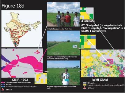
54 43

55 44

56 Comparing Global Products in India The comparison between FAO/UF global irrigated area map and GIAM10 km V2.0 highlights the distinct features of areas where the two maps: a) perfectly match (e.g., figure 19a in the Upper Ganges basin), b) broadly match (e.g., figure 19b in the Cauvery delta), and c) do not match at all (e.g., figure 19c in the Ganges delta). This illustration is a representative comparison of the two global irrigated area maps as we see similar trends in other places of the world. Figure 19 (a, b and c). Comparison of the two global irrigated area maps: GIAM10 km V2.0 and FAO/FU V

57 Irrigated Area Class Names At this stage it is useful to discuss the issues involved in final class labeling and the approach used in IWMI GIAM10 km V2.0. Classes were named based on a set protocol and rigorous methods (see figure 4) that had a clear classnaming convention (figure 9). In addition, the final class labeling (see figures 15 and 16) was also based on consultation with irrigation experts so that the class names represent the commonly understood meaning of a particular irrigation type. More generic and detailed names are provided in GIAM10 km-28 classes (figure 15), and simpler and broadly understood names are provided in GIAM10 km-8 classes (figure 16). The final class labeling was categorized under the following groups: irrigated, surface water, single crop, crop type or dominance irrigated, surface water, double crop, crop type or dominance irrigated, surface water, continuous crop, crop type or dominance The watering method (irrigated or rain-fed) and irrigation type (surface water, groundwater or conjunctive use) are determined based on the protocols and methods (see figure 4 and sections 4, 5 and 6). The single, double or continuous crop is determined based on the spectral signature for every class based on time-series satellite imagery (see example for class 1 and 4 in figure 20). The same classes 1 and 4 also occur in Iran showing somewhat different signature characteristics (in magnitude and timing of peaks and lows). Indeed, it is possible to get a cropping calendar for every pixel of irrigated area classes by simply clicking on any point on irrigated area class and looking through the time-series imagery of a mega-file as we have done in figures 20 and Figure 20. Single crop (red) and double crop (cyan) irrigation in the lower Ganges. 46

58 21. The final variable (crop type or dominance) in naming is based on groundtruth data and literature. This convention is repeated for groundwater and conjunctive use irrigation. In figure 15, classes 1-10 are surface water irrigation, classes are groundwater irrigation, and classes are conjunctive use irrigation. These classes were combined appropriately to produce the simplified eight-class irrigated area map (see figure 16). The class labeling process of one class has been discussed in detail. First, we go through a normal protocol (figure 8), methods (sections 5 and 6), and class naming convention (figure 9). In addition, the detailed approach to name a class is illustrated below for one class. Class 28 (figure 22) was labeled irrigated, conjunctive use, continuous crop, mixed crop in GIAM10 km-28 class map (figure 15). It occurs mainly in the Pampas of Argentina, which is predominantly rain-fed. However, different degrees of Figure 21. Double crop (left) and single crop (right) irrigation in Zayandeh and Rud. 47

59 Figure 22. Evaluation of GIAM for conjunctive irrigation. The rain-fed class with significant central pivot supplemental irrigation in the Pampas in Argentina. supplemental groundwater irrigation (e.g., pivots, drip) and some pumping from rivers also exist. Center-pivot irrigation is used in humid plains of Pampas to supplement rainfall (Maletta 1998, 1999). The spectral characteristics of the class show near continuous cropping, with AVHRR NDVI greater than 0.35 or more throughout the year (figure 22). Rainfall during May-September is low, averaging less than 40 mm per month (see figure 22) and is insufficient to sustain such high vegetation in an agricultural belt. The Pampas is a humid plain, which is very flat and is poorly drained. This and man-made obstacles such as roads and railroad embankments lead to flooding and waterlogging for months, favoring growth of weeds and natural pasture in the vicinity even during relatively dry spells (Maletta personnel communication). The long period of deficit rainfall and continuously high NDVI strongly imply some degree of irrigation. Evidence (Maletta personal communication) from the field suggests that center-pivot irrigation in the Pampas is mostly used for complementary irrigation while drip irrigation is used for horticulture. Maletta summarizes the situation: There is indeed a need to irrigate more, as witnessed by the fact that average yields (especially for maize) are quite below potential. But a) massive use of irrigation is not yet happening, b) aquifers may not support such an extensive use of underground water, and c) gravity irrigation is in general difficult due to very flat land, thus requiring pumping (which is not generally done) from the many streams flowing through the plains. The data from the Government administration ( show nearly 1.4 Mha are 48