Innovative Tools and Techniques in Identifying Highway Safety Improvement Projects: Technical Report

Transcription

1 TTI: Innovative Tools and Techniques in Identifying Highway Safety Improvement Projects: Technical Report Technical Report Cooperative Research Program TEXAS A&M TRANSPORTATION INSTITUTE COLLEGE STATION, TEXAS in cooperation with the Federal Highway Administration and the Texas Department of Transportation

2

3 1. Report No. FHWA/TX-17/ Title and Subtitle INNOVATIVE TOOLS AND TECHNIQUES IN IDENTIFYING HIGHWAY SAFETY IMPROVEMENT PROJECTS: TECHNICAL REPORT 7. Author(s) Ioannis Tsapakis, Karen Dixon, Jing Li, Bahar Dadashova, William Holik, Sushant Sharma, Srinivas Geedipally, and Jerry Le 9. Performing Organization Name and Address Texas A&M Transportation Institute College Station, Texas Sponsoring Agency Name and Address Texas Department of Transportation Research and Technology Implementation Office 125 E. 11 th Street Austin, Texas Technical Report Documentation Page 2. Government Accession No. 3. Recipient s Catalog No. 5. Report Date August Performing Organization Code 8. Performing Organization Report No. Report Work Unit No. (TRAIS) 11. Contract or Grant No. Project Type of Report and Period Covered Technical Report: September 2015 June Sponsoring Agency Code 15. Supplementary Notes Project performed in cooperation with the Texas Department of Transportation and the Federal Highway Administration. Project Title: Innovative Tools and Techniques in Identifying Highway Safety Improvement Projects URL: Abstract The Highway Safety Improvement Program (HSIP) aims to achieve a reduction in the number and severity of fatalities and serious injury crashes on all public roads by implementing highway safety improvement projects. Although the structure and main components of the Texas Department of Transportation s (TxDOT s) HSIP comply with relevant requirements, a review of modern safety assessment methods and tools revealed that there are several areas for improvement. As national safety assessment methods have evolved, legislation mandates that the use of safety performance methods be elevated. This research addresses how TxDOT can allocate funds in the most cost-effective manner; create a level playing field for all districts participating in the HSIP; promote district participation in the program; and minimize the amount of time and resources required to identify HSIP projects. To address these objectives, this study focused on improving and streamlining four (of six) components of the framework: a) network screening; b) diagnosis; c) countermeasure selection; and d) project prioritization. The researchers developed and applied a network screening process for roadway segments; conducted a pilot study for intersection network screening; developed and implemented a Crash Analysis and Visualization process that creates various informational products that display crash data and locations where certain types of safety countermeasures can be implemented; and developed a project prioritization spreadsheet. Among various improvements, the main benefits gained from using these tools include an increase in the number of HSIP projects identified by TxDOT districts by up to 57 percent and a reduction in the time and effort required to select projects by percent. 17. Key Words Highway Safety Improvement Program, HSIP, Network Screening, CAVS, Crash Reduction, Project Selection, Project Prioritization 19. Security Classif. (of this report) Unclassified Form DOT F (8-72) 20. Security Classif. (of this page) Unclassified 18. Distribution Statement No restrictions. This document is available to the public through NTIS: National Technical Information Service Alexandria, Virginia No. of Pages Price Reproduction of completed page authorized

4

5 INNOVATIVE TOOLS AND TECHNIQUES IN IDENTIFYING HIGHWAY SAFETY IMPROVEMENT PROJECTS: TECHNICAL REPORT by Ioannis Tsapakis, Ph.D. Associate Research Scientist Karen Dixon, Ph.D., P.E. Senior Research Engineer Jing Li, Ph.D., P.E. Assistant Research Engineer Bahar Dadashova, Ph.D. Associate Transportation Researcher William Holik, Ph.D. Assistant Research Scientist Sushant Sharma, Ph.D. Associate Research Scientist Srinivas Geedipally, Ph.D., P.E. Associate Research Engineer and Jerry Le Software Application Developer Report Project Project Title: Innovative Tools and Techniques in Identifying Highway Safety Improvement Projects Prepared in cooperation with the Texas Department of Transportation and the Federal Highway Administration August 2017 TEXAS A&M TRANSPORTATION INSTITUTE College Station, Texas

6

7 DISCLAIMER This research was performed in cooperation with the Texas Department of Transportation (TxDOT) and the Federal Highway Administration (FHWA). The contents of this report reflect the views of the authors, who are responsible for the facts and the accuracy of the data presented herein. The contents do not necessarily reflect the official view or policies of FHWA or TxDOT. This report does not constitute a standard, specification, or regulation. This report is not intended for construction, bidding, or permit purposes. The principal investigator of the project was Ioannis Tsapakis and Karen Dixon served as the co-principal investigator. The United States Government and the State of Texas do not endorse products or manufacturers. Trade or manufacturers names appear herein solely because they are considered essential to the object of this report. v

8 ACKNOWLEDGMENTS This research was conducted in cooperation with TxDOT and FHWA. The researchers would like to thank Corpus Christi District officials, who shared with researchers and other TxDOT districts information, data, files, and several ideas that were examined in this study. Specifically, the project team would like to thank Ismael Soto and his team for their innovative ideas and support. America Garza, Kassondra Munoz, Jacob Longoria, Mariela Garza, and Dexter Turner provided valuable help and advice throughout this project. The researchers also gratefully acknowledge the advice and assistance of Darren McDaniel and the other project advisors at TxDOT. Project team members met with numerous other individuals at TxDOT to gather and/or complement data and information needed for the analysis. They gratefully acknowledge the help and information received to complete this project. vi

9 TABLE OF CONTENTS Page List of Figures... ix List of Tables... xi List of Acronyms, Abbreviations, and Terms... xii Chapter 1. Introduction... 1 Chapter 2. Literature Review... 7 Introduction... 7 Safety Assessment Methods... 7 Network Screening... 7 Diagnosis Countermeasure Selection Economic Appraisal Project Prioritization Safety Effectiveness Evaluation Evolving Methods Current HSIP Practices and Tools Current HSIP Practices at TxDOT Other State HSIP Practices Lessons Learned and Areas for Improvement Chapter 3. Evaluation of Safety Assessment Methods and Tools Introduction Network Screening Applications Network Screening for Segments Network Screening for Intersections Project Selection and Prioritization Applications HSIP Project Prioritization Methods Project Prioritization Tools Chapter 4. Network Screening for Intersections A Pilot Study Introduction Data Preparation Intersection Data Crash Data Network Screening Step 1 Establish Focus Step 2 Establish Reference Populations Step 3 Apply Selected Performance Measures Step 4 Screening Method Step 5 Evaluation of Results Chapter 5. Network Screening for Segments Introduction Network Screening Process Step 1 Establish Focus Step 2 Identify Network and Establish Reference Populations vii

10 Step 3 Select Performance Measures Step 4 Select Screening Method Step 5 Screen and Evaluate Results Network Screening Products Data Tables Maps Chapter 6. Diagnosis and Countermeasure Selection Introduction Diagnosis Step 1 Review Safety Data Step 2 Assess Supporting Documentation Step 3 Assess Field Conditions Countermeasure Selection CAVS Products Development of CAVS Process Description Evaluation Chapter 7. Project Prioritization Introduction Project Prioritization Process and Tool Comparison between TxDOT and HSM Project Prioritization Processes Current TxDOT Project Prioritization Process Results Chapter 8. Conclusions and Recommendations Conclusions Recommendations References Appendix A HSM Elements Regression to the Mean Safety Performance Functions Crash Modification Factors Calibration Factor Appendix B State HSIP Information and Data Appendix C HSIP Tools Appendix D Intersection Network Screening Data and Results viii

11 LIST OF FIGURES Page Figure 1. HSIP Components and Relationship with SHSP (2) Figure 2. HSM Roadway Safety Management Process Explored in This Research (5) Figure 3. Illustration of the Sliding Window Method (7) Figure 4. Peak Search Method (7) Figure 5. Conceptual Example of EB Method Figure 6. TxDOT s HES Program Funding Process (17) Figure 7. Frequency of Programs Administered under State HSIPs Figure 8. Number of Programs per State Figure 9. Frequency of Project Identification Methodology Used Figure 10. Number of Project Identification Methodologies Used for All Programs Administered under a State HSIP Figure 11. Number of States that Evaluated SHSP Emphasis Areas Figure 12. Number of States that Evaluated Groups of Similar Types of Projects Figure 13. Number of States that Evaluated Systemic Treatments Figure 14. Percent Use of Ranking Methods Figure 15. Percent Use of Scoring Methods Figure 16. Intersection Data Collection Figure 17. Buffer Approach to Identify Intersection Related Crashes Figure 18. Overlapping Buffers Figure 19. National Safety Council Scale for Crash Severity (44) Figure 20. Network Screening Results of Pilot Study Area in San Antonio Figure 21. Main Steps of Network Screening Process for Roadway Segments Figure 22. Network Screening Flowchart for On-System Main-Lane Segments Figure 23. Legend of Network Screening Flowchart Figure 24. Zoomed-In View of Network Screening Flowchart (Part A) Figure 25. Zoomed-In View of Network Screening Flowchart (Part B) Figure 26. Zoomed-In View of Network Screening Flowchart (Part C) Figure 27. Zoomed-In View of Network Screening Flowchart (Part D) Figure 28. Zoomed-In View of Network Screening Flowchart (Part E) Figure 29. Zoomed-In View of Network Screening Flowchart (Part F) Figure 30. Zoomed-In View of Network Screening Flowchart (Part G) Figure 31. Example of Network Screening Results Figure 32. High Risk and Very High Risk Windows Figure 33. CAVS Process Figure 34. GE Layer Work Code 101 Install Warning Guide Signs (Fort Worth District) Figure 35. Zoomed-in View of Various Parts of Crash Attribute Table Displayed in a GE Layer Figure 36. Example of a Field Diagram Included in a Crash Report Figure 37. List of Feature Classes Contained in a File Geodatabase Figure 38. Main Steps of Diagnosis Process Figure 39. Main Steps of Countermeasure Selection Process ix

12 Figure 40. Main Steps of Project Prioritization Process Figure 41. Zoomed-In View of the IBCR Project Prioritization Process Figure 42. Screenshots of Project Prioritization Tool x

13 LIST OF TABLES Page Table 1. Performance Measures Included in FHWA s HSIP Online Reporting Tool Table 2. Programs Listed in the HSIP Report Template Table 3. Data Needs and Stability of Performance Measures Table 4. Strengths and Limitations of Performance Measures Table 5. Level of Effort Estimates for SPF Calibration and Development (30) Table 6. Relative Rank of Methods Used to Prioritize Projects Table 7. Project Selection and Prioritization Tools Table 8. Classification of Sample Intersections Table 9. Sample of Intersection Data Elements Table 10. Descriptive Crash Statistics Table 11. Calculations of Selected Performance Measures Table 12. Intersection Ranking Based on the Performance Measures Table 13. Number of Times an Intersection Was Selected as a High Priority Site Table 14. Weight Assigned to Each Performance Measure Table 15. Criteria for Identifying Similar Adjacent Segments Table 16. Roadway Groupings for Assessing Crash Risk Table 17. Strengths and Limitations of Using the Performance Measures Table 18. Attributes Included in Network Screening Spreadsheet Table 19. Summary Results and Improvement Achieved before and after Using Basic Visualization Products by Corpus Christi District Staff Table 20. Improvement Achieved before and after Using CAVS Products Statewide Table 21. Comparison of Projects Awarded Using the TxDOT Project Prioritization Approach and the IBCR Method Table 22. Projects Awarded Using the HSM and the TxDOT Approaches Table 23. States Using Advanced Project Identification Methodologies Table 24. How Local Roads Are Addressed as a Part of the HSIP Table 25. How Internal and External Partners Are Involved in the HSIP Table 26. Coordination Practices with Partners Involved in the HSIP Table 27. Programs Administered under the HSIP Table 28. Data Types Used within the HSIP Table 29. HSIP Project Identification Methodologies Table 30. How Projects Advance for Implementation Table 31. HSIP Project Prioritization Process Table 32. Types of Systemic Improvements Table 33. Process Used to Identify Countermeasures Table 34. Data Used to Capture Highway Safety Trends for the Last Five Years* Table 35. HSIP Tools by Agency Table 36. Sample Intersection Data Used in the Pilot Study Table 37. Network Screening Results of Pilot Study xi

14 LIST OF ACRONYMS, ABBREVIATIONS, AND TERMS A AADT ADT AASHTO AWR B B/C BCR BIKESAFE C CAVS CEAO CF CFR CMAT CMF CR CRF CRIS CRP CS CT DFO DOT EB EPDO FHWA GE GIS HAT HES HSCA HSIP HSM IBCR IHSDM ISS ITE K LOSS MAP-21 MEV MM MPO Incapacitating injury crash Annual average daily traffic Average daily traffic American Association of State Highway and Transportation Officials Adjusted weighted ranking Non-incapacitating injury crash Benefit-cost Benefit cost ratio Bicycle Safety Guide and Countermeasure Selection System Possible injury crash Crash Analysis and ViSualization County Engineers Association of Ohio Crash frequency Code of Federal Regulations Crash Mapping Analysis Tool Crash modification factor/function Crash rate Crash reduction factor Crash Records Information System Continuous risk profile Crash severity Crash type Distance from origin Department of Transportation Empirical Bayes Equivalent property damage only Federal Highway Administration Google Earth Geographic information system Hazard Analysis Tool Hazard Elimination Program Highway safety corridor analysis Highway Safety Improvement Program Highway Safety Manual Incremental benefit cost ratio Interactive Highway Safety Design Model Intersection safety score Institute of Transportation Engineers Fatal crash Level of service of safety Moving Ahead for Progress in the 21st Century Act Million entering vehicles Method of moments Metropolitan Planning Organization xii

15 NB NPV OASIS PACF PAWR PBCAT PEDSAFE PDO PEF PHV RHiNo RISE RSRAP RTM SAMS SHSP SII SLOSSS SPF SPIS TAZ TEV TOR TREDIS TRF TTI TxDOT usrap Negative binomial Net present value Oregon Adjustable Safety Index System Predicted average crash frequency Percent adjusted weighted ranking Pedestrian and Bicycle Crash Analysis Tool Pedestrian Safety Guide and Countermeasure Selection System Property damage only Project evaluation factor Peak hour volume Road-Highway Inventory Network Roadway improvement safety evaluation Resurfacing Safety Resource Allocation Program Regression to the mean Safety Analysis Management System Strategic Highway Safety Plan Safety improvement index Suggested list of surveillance study sites Safety performance function Safety priority index system Traffic analysis zone Total entering vehicles Time of return Transportation economic development impact system Traffic Operations Division Texas A&M Transportation Institute Texas Department of Transportation United States Road Assessment Program xiii

16

17 CHAPTER 1. INTRODUCTION The Highway Safety Improvement Program (HSIP) was established under the Safe, Accountable, Flexible, Efficient Transportation Equity Act: A Legacy for Users in 2005 and provided flexibility to states to target funds for their most critical safety needs. The Moving Ahead for Progress in the 21st Century Act (MAP-21) continued and refined the HSIP as a core federal-aid program (1). The goal of the program is to achieve a reduction in the number and severity of fatalities and serious injury crashes on all public roads by implementing highway safety improvement projects. To ensure that the HSIP is carried out in an organized and systematic manner, Texas (as well as every state department of transportation [DOT]) must develop, implement, and update a comprehensive, data-driven Strategic Highway Safety Plan (SHSP). The SHSP defines state safety goals and describes a program of strategies to improve all aspects of safety engineering, education, enforcement, and emergency medical services as stipulated in the United States Code (23 USC 148). Each state agency must also produce a program of projects or strategies to reduce identified safety problems and evaluate the SHSP on a regular basis. The SHSP remains a statewide coordinated plan developed in cooperation with a broad range of multidisciplinary stakeholders. State DOTs are required to allocate HSIP funds to various districts (and counties) based on criteria developed under the SHSP. The HSIP program funds are eligible to cover 90 percent of project construction costs. The remaining 10 percent of project construction costs must be covered by state or local participation. The code of federal regulations (CFR), 23 CFR 924, mandates a formalized HSIP process that includes three major components: planning, implementation, and evaluation (2). The planning aspect involves analyzing data and identifying safety problems, determining appropriate countermeasures, and selecting and prioritizing projects. Once HSIP project funding is secured, projects are designed and constructed during the implementation phase. In the evaluation phase, state agencies determine the effectiveness of individual project locations, countermeasures, and programs. The evaluation results are then taken into consideration and used during planning to make adjustments and improve the entire HSIP process, as needed. Figure 1 shows the three components, their processes, and their relationship with the SHSP. In compliance with federal regulations, the Traffic Operations Division (TRF) of the Texas Department of Transportation (TxDOT) developed and currently administers TxDOT s HSIP (3). TRF requests proposed HSIP projects from districts through an annual statewide program call. Projects funded in the HSIP are limited to improvements that address the serious crash types identified in the most current Texas SHSP (4). All eligible proposed highway safety projects are subjected to a benefit-cost (B/C) analysis. 1

18 Figure 1. HSIP Components and Relationship with SHSP (2). While the structure and main components of TxDOT s HSIP are in line with relevant requirements, certain processes that take place within HSIP components can be improved and optimized. As national safety assessment methods have evolved, legislation mandates that the use of safety performance methods be elevated (1). At one time, basic safety criteria, such as crash frequency and crash rate, helped identify candidate safety improvement locations. Today, the profession recognizes that though crashes are rare events, it is possible to predict locations where crashes are likely to occur. The increased use of advanced safety assessment methods and tools in the state will help to determine locations and safety improvements that have the greatest potential to reduce fatal and injury crashes while minimizing the influence of unstable crash trends over many years. The latest safety assessment methods explicitly consider unique facility geometric features that may contribute to a crash and enable the identification of systemic measures that will result in widespread, statewide crash reductions. Some of the safety 2

19 assessment methods are included in the Highway Safety Manual (HSM) (5) and TxDOT s Roadway Safety Design Workbook (6). The current HSIP project selection process at TxDOT can be improved by implementing consistent site selection procedures among districts and using innovative tools to systematically screen candidate sites for safety improvement. The improvement can also relieve TxDOT from large demands on staff manpower resources for the HSIP program. This research evaluated the applicability of modern and evolving safety assessment methods and developed innovative tools and techniques based upon the results. These innovative tools and techniques will allow TxDOT to: Allocate funds in the most cost-effective manner. Create a level playing field for all districts participating in the HSIP and promote district participation in the process. Minimize the amount of time and resources required to identify HSIP projects. To accomplish this goal, the Texas A&M Transportation Institute (TTI) researchers adopted the HSM s Roadway Safety Management Process, which includes six components (Figure 2) explained below (5): Network Screening Scan network and identify high risk locations and sites. Diagnosis Review past studies and road characteristics to identify crash patters and understand causes of crashes and safety concerns. Countermeasure Selection Identify risk factors contributing to crash causes and select site-specific countermeasures to reduce crash frequency and severity. Economic Appraisal Compare anticipated benefits and project costs of selected countermeasures. Project Prioritization Rank safety improvement projects based on their potential to achieve the greatest reduction in the number and severity of crashes. Safety Effectiveness Evaluation Assess the effectiveness of a safety improvement project, group of similar projects, and the entire program. 3

20 Figure 2. HSM Roadway Safety Management Process Explored in This Research (5). Researchers tailored this cyclical roadway safety management process to TxDOT s needs, objectives, and HSIP requirements and used it as a framework for conducting this study. This process is hereafter referred to as the general safety management framework or simply general framework. Considering the given timeframe and budget of this project, it would not be feasible to develop tools and techniques for all six processes. To maximize the anticipated benefits of the project deliverables to TxDOT, researchers focused on improving and streamlining four processes that were identified as critical elements in TxDOT s HSIP and could be immediately enhanced by developing new methods and tools. These processes are highlighted in a red rectangle in Figure 2 and include: a) network screening; b) diagnosis; c) countermeasure selection; and d) project prioritization. The remaining chapters of this report describe the activities performed to address the research objectives and documents how these four processes of the general framework can be improved: Chapter 2: Literature Review This chapter provides a literature review that covers traditional and evolving safety assessment methods, state HSIP practices, and tools. Chapter 3: Evaluation of Safety Assessment Methods and Tools This chapter describes the work performed to evaluate the applicability of modern safety assessment methods and tools at TxDOT. Chapter 4: Network Screening for Intersections A Pilot Study This chapter describes a case study of intersection network screening that was applied to a sample of 4

21 intersections in northern San Antonio. The network screening process can be applied in the future to all intersections in Texas, provided that intersection-related data are collected and gathered. Chapter 5: Network Screening for Segments This chapter presents a practical, sustainable, and streamlined network screening process for roadway segments. This process was applied to all on-system roads in Texas and can be used in the future by all TxDOT districts to support the HSIP project identification process. Chapter 6: Diagnosis and Countermeasure Selection This chapter describes the steps and key elements needed to identify crash patterns, causes of collisions, and roadway characteristics and then use this information to select appropriate countermeasures. It also presents a Crash Analysis and ViSualization (CAVS) process and the resulting products that TTI developed to enhance both the diagnosis and countermeasure selection processes at TxDOT. The CAVS products were used for testing purposes by TxDOT districts during the 2016 and 2017 HSIPs. Chapter 7: Project Prioritization This chapter describes a project prioritization process and a supporting spreadsheet tool that incorporates an incremental benefit cost ratio (IBCR) method, which is compared against TxDOT s existing project prioritization approach. Chapter 8: Conclusions and Recommendations This chapter provides conclusions and recommendations stemming from the work performed, research results, tools developed and tested, and various lessons learned throughout this project. 5

22

23 CHAPTER 2. LITERATURE REVIEW INTRODUCTION This chapter provides a literature review that covers the following: Traditional, modern, and evolving safety assessment methods that can be used to support HSIP processes. Current state of practice at TxDOT, HSIP processes at other state DOTs, general trends, and various tools used by transportation agencies nationwide. Lessons learned, gaps, and areas for improving existing TxDOT s HSIP processes and practices. SAFETY ASSESSMENT METHODS This section provides a synthesis of traditional, modern, and evolving safety assessment methods that are separately presented for each of the six processes included in the general safety management framework presented in Chapter 1 (Figure 2). Network Screening The network screening process includes ranking sites from most likely to least likely to realize a reduction in the number and severity of crashes if countermeasures are implemented. Researchers reviewed existing and evolving methods for network screening and summarized them in the following subsections. Highway Safety Manual Network screening is the first process in the framework, which includes five major steps: 1. Establish the goal and intended outcome of the network screening process. 2. Identify the network and establish reference population (e.g., segments, guardrails). 3. Select performance measures. The HSM provides a total of 13 performance measures (Table 1) that can be used to evaluate the potential to reduce crash frequency and severity. These measures are also called project identification methodologies in the Federal Highway Administration s (FHWA s) HSIP online reporting tool. 4. Select screening method. The HSM provides the following methods: o Simple ranking method. In this method, the sites under consideration are ranked based on the values of selected performance measures. This method can be applied to nodes, segments, or facilities (i.e., combination of nodes and segments). 7

24 o Sliding window method. In this method, a window of a certain length is conceptually moved along a study segment from one end to another at specified increments. The selected performance measures are then calculated for each position of the window. From all the windows analyzed, the windows are ranked based on the values of performance measures. Figure 3 shows an example of conducting the sliding window method using a window length of 0.3 miles and an increment distance of 0.1 miles. This method only applies to segments. o Peak searching method. In this method, the individual roadway segments are divided into windows of similar length. Figure 4 illustrates the main steps of the method. The roadway is first subdivided into 0.1-mile windows, with the exception of the last window, which may overlap with the previous window. The selected performance measures are then calculated for each window, and the resulting value is subject to a desired level of precision. If none of the 0.1-mile segments meet the desired level of precision, the segment window is increased to 0.2 miles, and the process is repeated until a desired precision is reached or the length of the window equals the entire segment length. For example, if the desired level of precision is 0.2, and the calculated coefficient of variation for each segment is greater than 0.2, then none of the segments meet the screening criterion and the segment length should be increased. 5. Screen and evaluate results. The outcome of the analysis is a list of sites ranked based on the value of the selected performance measure(s). The HSM indicates that applying multiple performance measures can be useful for this type of analysis. 8

25 Table 1. Performance Measures Included in FHWA s HSIP Online Reporting Tool. Performance Measure Crash Frequency Crash Rate Equivalent Property Damage Only (EPDO) Average Crash Frequency Relative Severity Index Critical Rate Excess Predicted Average Crash Frequency (PACF) Using Method of Moments (MM) Level of Service of Safety (LOSS) Excess PACF Using Safety Performance Functions (SPFs) Probability of Specific Crash Types Exceeding Threshold Proportion Excess Proportion of Specific Crash Types Expected Average Crash Frequency with Empirical Bayes (EB) Adjustment EPDO Average Crash Frequency with EB Adjustment Excess Expected Average Crash Frequency with EB Adjustment Description Number of crashes for a given road segment or intersection over a specified analysis period. Sites with higher number of total crashes (or a particular severity) are ranked first. Number of crashes per million miles of travel. Crash rate analysis typically uses exposure data in the form of traffic volumes or roadway mileage to determine relative safety compared to other similar facilities. Weighting factors related to the societal costs of fatal, injury, and property damage only (PDO) crashes are applied to crashes to develop an EPDO score that considers both frequency and severity of crashes. Each crash type is assigned an average monetary cost and the total average cost of all crashes at a site is compared to the average crash cost of the reference population. The critical crash rate is calculated for each site and compared to the observed number of crashes. If the observed number of crashes for the given site is higher than the critical rate, this site is marked for further analysis. The observed crash frequency at each site is modified and compared to the average crash frequency of the reference population. Analysts can adjust sites crash frequency to partially account for regression to the mean (RTM) effects. The observed crash frequency and/or severity are compared to the predicted mean value of the reference population. The difference between these two values is ranked by a performance measure that ranges from LOSS I to LOSS IV. LOSS I indicates low potential for crash reduction, while LOSS IV indicates the highest potential for reducing the number of crashes. Difference between the observed crash frequency and the predicted crash frequency derived from an appropriate SPF. The probability that the long-term proportion of a specific crash type exceeds a threshold proportion. Sites are prioritized based on the probability that the true proportion of a particular crash type or severity is greater than a prescribed threshold proportion. Difference between the observed proportion of a specific crash type for a site and the threshold proportion for the reference population. The expected number of crashes is calculated by a calibrated SPF and then is adjusted by the observed number of crashes using the EB method. The expected number of crashes derived by a calibrated SPF is modified by the observed EPDO crashes using EB, which is then weighted based on crash severity and the EPDO cost. This method assigns weighting factors to crashes by severity to develop a single combined frequency and severity score per location. The weighting factors are calculated relative to PDO crashes. The expected crash frequency derived from an SPF is weighted with the observed crash frequency using the EB method and then is compared to the expected crash frequency. 9

26 Figure 3. Illustration of the Sliding Window Method (7). 10

27 Figure 4. Peak Search Method (7). 11

28 Systemic Safety Project Selection Tool MAP-21 placed emphasis on performance measures and encouraged states to incorporate systemic approaches into their SHSP. In response to MAP-21 requirements, FHWA developed the systemic safety project selection tool to assist agencies in applying a systemic approach to improve safety system-wide (8). The systemic approach is not intended to replace the traditional site-specific approach, but instead, supplement the traditional approach. The systemic safety planning process consists of four stages. Each stage may be scaled based on the availability of technical resources and data. The first two stages cover the network screening process as described below and may also cover the diagnosis and project prioritization processes: Identify focus crash types and risk factors: o Identify most frequently observed severe crash types using historical crash data (9). o Proceed to the identification and selection of focus facilities based on the identified focus crash types. Crash tree diagrams can be used for this purpose to simply illustrate the categorization of crashes. It was indicated in the report that crash tree analysis should at least include separation by urban and rural, state and local, node and segment, segment type, and intersection control type. o Identify and evaluate the most common risk factors based on the focus crash types and facilities identified from the previous two steps. After identifying potential risk factors, the analyst should evaluate the factors to determine whether the correlation between the factors and future crash potential is significant. The methods of evaluating risk factors are: Descriptive statistics can be used to identify major risk factors that caused severe crashes. One way is to compare the proportion of locations with certain characteristics with the percentage of severe crashes at the same locations. Another way is to compare the crash density of locations with and without certain characteristics. Crash modification factors/functions (CMFs) from published research. Quantitative CMFs represent the estimated change in crash frequency after implementing safety treatments. A CMF is computed as the ratio of the expected crash frequency at a site where the treatment has been implemented to the expected crash frequency at a site where the safety treatment has not been implemented. The FHWA-maintained CMF Clearinghouse website provides a comprehensive and searchable database of published CMFs for agencies and researchers to conduct safety analysis (10). The available CMFs are classified using various criteria, such as star quality rating, crash type, crash severity, roadway type, area type, intersection type, traffic control, etc. Users can learn how to select appropriate CMFs for their analyses through the user s guidance. 12

29 Screen and prioritize candidate locations: o Select roadway elements to review and split the selected sites into homogenous segments having consistent cross-sections. o Conduct risk assessment by characterizing the potential for severe focus crashes at the selected elements (e.g., segments, horizontal curves, intersections). Descriptive statistics such as severe crash density with/without risk factors can be used to perform the assessment. o Prioritize roadway elements based on the presence of selected risk factors. This activity can be done using the descriptive statistics estimated in the previous activity. Pedestrian/Bicycle Safety Guide and Countermeasure Selection System FHWA published safety guides and countermeasure selection systems for pedestrians and bicyclists independently. Both safety guides and countermeasure selection systems (i.e., Pedestrian Safety Guide and Countermeasure Selection System [PEDSAFE] and Bicycle Safety Guide and Countermeasure Selection System [BIKESAFE]) are intended to provide practitioners with tools for improving safety and mobility of pedestrians and bicyclists. The online tools (located at provide users with a list of possible engineering, education, or enforcement treatments to improve pedestrian/bicyclist safety and/or mobility based on user input about these locations. The general steps used for both network screening and diagnosis are: 1. Identify and analyze factors that affect pedestrian/bicyclist safety. 2. Analyze pedestrian/bicyclist crash data. 3. Establish crash-related and/or performance-based goals. 4. Select and implement countermeasures that address pedestrian/bicycle safety: Diagnosis o 68 unique engineering countermeasures and treatments for improving pedestrian safety. o Eight countermeasures for improving bicyclist safety. Diagnosis is the second process of the general framework. It involves reviewing past studies and roadway/roadside characteristics to identify crash patterns and better understand causes of crashes and safety concerns that may need to be assessed further. Diagnosis, together with network screening, help identify locations and segments that are likely to realize the greatest safety benefits from implementing countermeasures. The methods used in the diagnosis process are summarized in the following subsections. 13

30 Highway Safety Manual The diagnosis process included in the general framework covers three major steps: Crash data review. This step reviews descriptive statistics of crash conditions and locations that help reveal crash trends. The HSM recommends several illustrative tools for data trend analysis, such as collision diagrams, condition diagrams, and crash mapping. Assess supporting documentation. This step gathers information on site-specific infrastructure improvements, traffic operations, geometry, traffic control, travel modes, and relevant public comments. The HSM provides a list of questions that can be used to conduct this assessment. Field conditions assessment. This step visits the subject sites and evaluates the local roadway/roadside conditions. The information gathered from this assessment complements the findings from the first two steps. For a multimodal, multidisciplinary perspective, field investigation becomes more important. Systemic Safety Project Selection Tool The process of diagnosis in the Systemic Safety Project Selection Tool was integrated with the network screening process. The activities associated with diagnosis include: Identify and evaluate the most common risk factors. Select locations or elements of roadway system to review. Conduct risk assessment by characterizing the potential for severe focus crashes at the selected locations or elements. Refer to the subsection of Systemic Safety Project Selection Tool under Network Screening for more details about these activities. Pedestrian/Bicycle Safety Guide and Countermeasure Selection System Likewise, the diagnosis process included in the PEDSAFE/BIKESAFE was integrated with the network screening process. The activities associated with diagnosis include: Identify and analyze factors that affect pedestrian/bicyclist safety. Analyze pedestrian/bicyclist crash data. Countermeasure Selection The countermeasure selection process involves identifying crash contributing factors and selecting appropriate site-specific countermeasures to address potential safety problems and 14

31 concerns. The following subsections present a summary of the existing methods for identifying and selecting countermeasures. Highway Safety Manual The countermeasure selection process contains three major steps: 1. Identify factors contributing to the cause of crashes at the subject site. Factors contributing to different crash types can be divided into three categories: roadway, vehicle, and human factors. 2. Identify countermeasures that may address the contributing factors. The HSM and the CMF Clearinghouse provide quantitative CMFs for various countermeasures or treatments, which can be used to identify and select appropriate countermeasures. 3. Assess benefits of countermeasures. This step uses predictive methods including SPFs and CMFs to assess the benefits in terms of change in crash frequency. Once the expected changes in crash frequency are estimated, these benefits are then converted to monetary benefits by considering societal costs of crashes. Systemic Safety Project Selection Tool The major steps included in the Systemic Safety Planning Process for countermeasure identification and selection are similar to the steps provided in the HSM: 1. List cost-effective countermeasures based on the selected focus crash types and candidate locations. Various sources can be used for identifying an initial list of safety countermeasures, such as the National Cooperative Highway Research Program Report 500 series (11), the HSM, the CMF Clearinghouse, state SHSPs or local safety plans, FHWA s illustrated guide sheets for 77 intersection countermeasures (12), and TxDOT s existing maintenance program. 2. Evaluate and screen candidate countermeasures based on the effectiveness of countermeasures in reducing focus crashes, implementation and maintenance costs, and consistency with agency s policies, practices, and experiences. B/C analysis can be performed in this step. A detailed B/C analysis conducted by the Rutgers Center for Advanced Infrastructure and Transportation Safety Resource Center for Salem County was included in the research report. The analysis contains the following activities: o Use SPFs and CMFs to estimate the benefits of implementing countermeasures (change in crash frequency). o Calculate the net present value (NPV) of implementation and maintenance costs and estimate the benefit-cost ratio (BCR) for a specific countermeasure. o Prioritize countermeasures based on the BCR. 15

32 3. Select countermeasures for deployment. This step involves using the prioritized list of countermeasures from the previous step to create safety projects for deployment. Pedestrian/Bicycle Safety Guide and Countermeasure Selection System The third step of PEDSAFE and BIKESAFE deals with the selection and implementation of countermeasures that address pedestrian/bicyclist safety. After identifying the objective/crash type and the necessary treatment, applicable countermeasures are determined from a list of countermeasures provided in the PEDSAFE/BIKESAFE Guide. Each countermeasure includes a description of the treatment or program, purpose, considerations, cost estimates, and a list of case studies that have implemented the countermeasure of interest. Economic Appraisal After identifying locations with potential for crash reduction and selecting countermeasures, the next step is to compare candidate projects by performing an economic appraisal. Although many factors and objectives may play a role in this process, transportation safety professionals generally select and prioritize projects based on what will yield the greatest benefits within the available funding constraints. The following subsections describe economic appraisal methods identified by researchers. Highway Safety Manual The methods of conducting economic evaluation described in the HSM include: B/C analysis methods compare the benefits associated with a countermeasure, expressed in monetary terms, to the cost of implementing the countermeasure. The goal is for the benefits to be greater than the costs. B/C analysis provides a quantitative measure to help safety professionals prioritize countermeasures or projects and optimize the return on investment. o The NPV method assesses the difference between the discounted costs and discounted benefits of a safety improvement project. The NPV method is used to determine which countermeasure(s) provides the most cost-efficient means based on the countermeasure(s) with the highest NPV. It can also determine if a project is economically justified (i.e., NPV greater than zero). o A BCR is the ratio of the present value of the benefits of a project to the present value cost of the project. A project with a BCR greater than 1.0 is considered economically justified. However, the BCR is not applicable for comparing various countermeasures or multiple projects at various sites; this requires an incremental B/C analysis. Cost effectiveness analysis methods are used in situations where it is not possible or practical to monetize countermeasure benefits. Cost-effectiveness is calculated as the amount of money invested to implement a countermeasure divided by crash reduction. A cost-effectiveness index can be calculated as the ratio of present value cost divided by this cost-effectiveness measure. This method does not account for reductions in fatal crashes as opposed to injury crashes and whether a project is economically justified. 16

33 The cost of implementing countermeasures involved in these methods should consider various factors, such as right-of-way acquisition, construction material costs, grading and earthwork, and utility relocation. Systemic Safety Project Selection Tool The Systemic Safety Project Selection Tool performs economic appraisal through the project development process. Safety projects are developed by providing a detailed site description (e.g., route number, mile point, intersecting roadway, and segment terminal), identifying the specific countermeasure selected, estimating the implementation cost, and summarizing how the site scored with the risk factors. After the countermeasures for safety investments are selected, agencies decide how to most efficiently bundle projects into a design package for contract letting. Project Prioritization The goal of project prioritization is to sort candidate safety improvement projects by conducting a ranking or optimizing analysis. The following subsections describe project prioritization methods identified from the literature. Highway Safety Manual For project prioritization, the HSM provides three single-objective prioritization methods as summarized below: Ranking by economic effectiveness measures. This is the simplest project prioritization method. Examples of ranking measures are project costs, monetary value of project benefits, total number of crashes reduced, number of fatal and injury crashes reduced, NPV, and cost-effectiveness index. Since these methods do not account for competing priorities, budget constraints or other impacts, they may not yield the best return on investment. Incremental B/C analysis ranking. This method is an extension of the BCR method. The BCR of the individual safety improvement projects are the starting point for an incremental B/C analysis. If two projects have the same cost, the project with the greater benefit should be selected. Optimization methods. These methods are used to identify a project that will maximize benefits within a fixed budget and other constraints. They are most effective if one needs to determine the most cost-effective set of improvement projects that fit the budget. Optimization methods such as linear programming, integer programming, and dynamic programming are similar to incremental B/C analysis and also account for budget constraints. Multiobjective resource allocation is another optimization method, which incorporates nonmonetary elements, including decision factors not related to safety, into the prioritization process. 17

34 Systemic Safety Project Selection Tool The Systemic Safety Project Selection Tool prioritizes selected safety improvement projects by identifying implementation sequences. The prioritization is risk based and also considers other factors such as funding, time constraints, expected crash reduction, efforts needed for public outreach, environmental and right-of-way constraints, and other programmed projects. Safety Effectiveness Evaluation The project evaluation process focuses on determining the effectiveness of a safety improvement project, groups of similar types of projects (or countermeasures), and the entire program. The following subsections summarize the existing methods for safety project evaluation. Highway Safety Manual According to the framework, the process of safety effectiveness evaluation may include: Evaluating a single project at a specific site. Evaluating a group of similar projects. Evaluating a group of similar projects to develop a CMF for a countermeasure. Assessing the overall safety and cost effectiveness of specific types of projects or countermeasures. This project evaluation analysis can use the following methods: Observational before/after studies. Observational before and after studies are a common and preferred method for evaluating the safety effectiveness of a project. These studies use crash and traffic data for the periods (e.g., 3 years) before and after the countermeasure implementation. Since the treatment sites are typically selected based on high crash frequency, applying this method can have some drawbacks due to the selection bias (i.e., sites are not randomly selected). Three methods are used to minimize site selection bias: the EB method, the SPF method, and a comparison group method. Among these methods, the EB method is the most commonly used. To assess the performance of the selected treatment, the EB method weights the predicted crash frequency together with the crash frequency observed at the site after the implementation of the treatment. This measure is labeled as Expected Average Crash Frequency (NN EEEEEEEEEEEEEEEE ). One reason that EB is preferred over the other before-after methods is that it explicitly adjusts the estimate of expected crashes to counter potential RTM bias by shifting the expected crash frequency toward the observed frequency using the SPFpredicted number of crashes (Figure 5). The EB method might not be optimal to certain situations since it requires a large number of sites (or observations) to evaluate countermeasure effectiveness. As an alternative, full Bayesian methods may be more appropriate for these before-after analyses; however, the application of full Bayesian methods is considerably more complex than that used for EB assessments. 18

35 Observational cross-sectional studies. In cross-sectional studies, data are gathered from similar sites (e.g., rural two-lane roads with horizontal curvature belonging to certain range) where the treatment had been applied to only a subset of the locations. The crash frequencies at the study sites (with and without treatment of interest) are compared to evaluate the safety effectiveness of the treatment. Cross-sectional methods are applied when: o Treatment installation date is not available. o Crash and traffic volume data for the period prior to installation is not available. o The evaluation needs to account for interactive effects of geometric characteristics. Experimental before/after studies. In experimental before and after studies, the sites with similar characteristics are divided into treatment and non-treatment groups, and the countermeasure is implemented to the sites in the treatment group. One of the main advantages of this method is that by randomly selecting the sites, the selection bias is minimized. 30 Observed Number 25 Expected Number Using EB Crash Frequency SPF Predicted Number from SPF AADT Systemic Safety Project Evaluation Tool Figure 5. Conceptual Example of EB Method. The last element of the Systemic Safety Project Selection Tool is the project evaluation tool. This tool is relatively new, so the evaluation process framework has not yet been fully described. The systemic safety evaluation tool uses severe crash history and risk factors to evaluate the safety performance considering the following three levels: 19

36 Output: At this initial level, agencies check the general outputs (e.g., implementation of planned systemic program, distribution of funding, and effective selection of countermeasures), and review their funding decisions annually and the consistency of the selected improvements. Focus crash type: At the second level, agencies conduct evaluations to estimate the decreasing trend in the number of crashes. The types of data used in the analysis depend on the geographic scale of the analysis (e.g., individual locations or system-wide analysis). For individual location safety analysis, data should include crash information of at least three years, roadway characteristic data, and traffic volume information. For system-wide safety analysis, the tool requires region-wide and state-wide data. Countermeasure performance: At the third level, agencies assess the effectiveness of countermeasures to assist with funding decisions for a specific project. This process may be carried out using the EB method to account for RTM, multivariate regression to account for more than one independent variable, or confidence tests to account for the statistical reliability of results. Evolving Methods In addition to abovementioned methods, researchers also reviewed a couple of evolving methods that include: Causal inferences from the HSM predictive methods assume that the counterfactual crash frequency (i.e., the crash frequency that would have been observed if the countermeasure had not been applied, can be reasonably estimated from the prediction of a base model). In causal models, an explicit treatment to the causal relationship is assumed. The effect of the countermeasure is then estimated by comparing the counterfactual crash frequency with the observed crash frequency. One of the casual inference models is Rubin s Causal Model (13) that is based on defining a set of potential observations for each population of observed crash frequency and unobserved counterfactual crash frequency. The effect of a treatment is then studied by employing non-randomized data selected from potential observations. Rubin s Causal Model employs a propensity score to mimic the random selection method. The propensity score is a scalar summary of a set of multiple potentially confounding covariates. In other words, using propensity scores, this method implicitly controls for confounding variables (i.e., variables that completely or partially correlate to an outcome and a risk factor). Causal inference models and propensity score matching methods are promising alternative methods to HSM predictive methods, particularly when dealing with crash severity data. However, few studies are available of this application on safety data. Epidemiological case-control studies are used to distinguish the effect of a selected countermeasure from the effects of other affecting factors. These types of studies are generally preferable to cross sectional methods (14, 15, 16). Case-control studies based on odds ratios can be used as an estimate of safety effectiveness of a treatment. It is argued that odds-ratio-case-control methods have several advantages compared to alternative safety evaluation methods (14) since they are able to study rare events, 20

37 evaluate multiple risk factors from a single sample, and they can control for confounding variables. However, as odds-ratio-case-control studies deal primarily with binary variables (crash occurs or does not occur) or binomial variables, they can only account for the probability of the crash occurrence relative to the sampling scheme. This perceived limitation can be addressed by defining binary categories (more than 10 crashes occur or 10 or fewer occur). Although potentially attractive, the application of this alternative to crash data is not wide spread and its implications are often misconstrued. CURRENT HSIP PRACTICES AND TOOLS This section documents current HSIP processes and tools used at TxDOT and other state agencies. To collect this information, researchers reviewed HSIP manuals, SHSPs, guidebooks, published reports, and other relevant documents. Researchers also reviewed state HSIP reports submitted to FHWA in 2015 and collected additional information to identify innovative HSIP tools. Current HSIP Practices at TxDOT This subsection describes the current state of practice at TxDOT, including the current structure and main processes of the HSIP, as well as the data and tools used by TxDOT staff to perform various HSIP activities. HSIP Structure and Processes The Texas HSIP includes a safety construction program called Hazard Elimination program (HES) that is part of the TxDOT Unified Transportation Program (Category 8) (17). HES focuses on construction and operational improvements on and off the state highway system. TRF works with districts to develop projects and identify potential highway safety improvement projects to be constructed when federal HSIP funds are available. These projects may range from spot-safety improvements and upgrading existing conditions to new roadway construction. Some of the objectives of HES projects are to correct or improve high-hazard locations; eliminate or treat roadside obstacles; improve highway signing and pavement markings; and install traffic control or warning devices at hot-spot locations. Figure 6 illustrates the funding process for the HES program. 21

38 Figure 6. TxDOT s HES Program Funding Process (17). Step 1 involves selecting safety emphasis areas using TxDOT s most recent (2014) SHSP (4). The 2014 SHSP includes 19 safety issues that have been grouped into four emphasis areas: crash type and location, system users, driver behavior, and system administration. To address some of these emphasis areas, the 2017 HSIP focuses on nine categories of work that include the following: 22

39 Barriers and Safety Treat Fixed Objects Adding or upgrading a barrier or metal beam guard fence to safety treat a fixed object or drainage structures. Curve Constructing improvements on horizontal curves to prevent run-off-the-road and head-on crashes. Grade Separation Constructing a vertical separation of a highway intersection (conventional diamond interchange). Intersection Improvements to an intersection, other than a grade separation. Off-System Any safety improvement to a road off the state highway system, which addresses an emphasis area in the SHSP. Pedestrians Construct improvements to prevent pedestrian crashes. Rumble Strips Adding edgeline or centerline rumble strips to a highway to prevent runoff-the-road and head-on crashes. Widen Increasing paved surface width of rural highways with current pavement width less than 24 ft and annual average daily traffic (AADT) greater than or equal to 400 vehicles per day to provide from 26 ft to 28 ft of paved surface width. HSIP Miscellaneous Safety Any safety improvement that addresses an emphasis area in the SHSP but is not categorized in one of the other eight categories. In Step 2, TRF identifies potential project locations, and Step 3 districts perform feasibility analysis and ensure countermeasures have not been implemented or scheduled for construction. In Step 4 and Step 5, districts work with area offices and local governments to identify countermeasures by combining crash and roadway information and applying engineering judgement. After countermeasures and project limits are determined, TxDOT engineers estimate project costs including a BCR, known as the Safety Improvement Index (SII). The SII was established in 1974 and revised in Currently, it is used for safety project prioritization purposes (18). In its most basic form, the SII is the ratio of the cost of preventable crashes that occurred at a particular location or roadway segment to the cost of constructing a safety improvement at that location or segment. Projects with an SII greater than or equal to one are considered cost-effective, and those with an SII of less than one are not eligible for funding under the existing HSIP. TxDOT s HSIP requires the use of three years of crash data to estimate the SII for every candidate project submitted to the program. The SII formula is: SS = RR(CC ffff + CC ii II) YY QQ = AA aa AA bb AA bb MM LL SS 23

40 BB = SS QQ 1.06 LL + SS + ii=2 1 QQ + (ii 1)QQ ii SSSSSS = BB CC where, S = Annual savings in preventable crash costs. R = Crash reduction factor. F = Number of preventable fatal and incapacitating injury crashes over a period of three years. I = Number of preventable non-incapacitating injury crashes over a period of three years. Cf = Average cost of a fatal or incapacitating injury crash based on the comprehensive cost figures provided by the National Safety Council. Ci = Cost of a non-incapacitating injury crash. Y = Number of years (three) of crash data. M = Change in annual maintenance costs for the proposed project relative to the existing situation. Q = Annual change in crash cost savings. Aa = Projected AADT at the end of the project service life. Ab = AADT during the year before the project is implemented. L = Project service life. B = Present worth of project benefits over the service life of the project. C = Initial cost of the project (17). As a ratio of benefit to cost, the SII was designed as a comparison device for project prioritization and may not be fully suitable as a measure for independent projects. In addition, the SII formula provides no evaluation of the appropriateness of the type of construction. Because the SII is a critical part of the safety site selection procedure, it is likely that some district staff are not aware of SII limitations that could potentially result in a suboptimal selection of safety countermeasures or project limits. Though this formula targets key safety needs, the results from this formula are only as reliable as the quality of the input information (i.e., accuracy of reduction factors) and the types of variables considered. Past research has shown that the SII is a robust formula (19), yet it predates recent advances in safety assessment methodologies that account for more variables such as geometric characteristics, roadway type, and traffic volume. Evaluating safety countermeasures using historical crash data and other regional or national SPFs can strengthen the project identification process at TxDOT. After a SII is estimated for every candidate project, HSIP reports are prepared and submitted along with other backup data to TRF as described in Step 6. In Step 7, TRF determines whether the submitted projects meet HSIP eligibility criteria including data accuracy and conformance with design standards. In Step 8, TRF prioritizes the candidate projects based on the SII and the availability of funds. TRF notifies districts about the selected projects in Step 9. Steps 10 through 24

41 13 involve several design, implementation, and budgeting activities that typically take place prior to project letting and construction. These activities are out of the scope of this research, so they will not be covered herein. Data and Tools Used at TxDOT As part of a SHSP, a state must implement and update a crash data system with the ability to perform safety problem identification and countermeasure analysis. In 2007, TxDOT took over the responsibility of collecting crash data from the Texas Department of Public Safety. Since then, TRF has been responsible for the management and maintenance of the Crash Records Information System (CRIS). CRIS is the official state database for traffic crashes occurring in Texas. Each TxDOT district has licensed staff who have access to CRIS (17). CRIS contains several tools designed to assist TxDOT staff in viewing, analyzing, and extracting crash data. For example, MicroStrategy is an interactive business intelligence platform, embedded into CRIS, and used for data reporting and analysis purposes (20). MicroStrategy allows users to extract and process crash data, filter for specific crash attributes, analyze trends, perform forecasting, create scorecards and dashboards, and generate user-defined reports, among others. CRIS also has a basic mapping system that is commonly used by districts to retrieve crash and roadway data that are often needed for completing HSIP project submission reports. In addition to CRIS, TxDOT officials occasionally use other web-based platforms, such as the statewide planning map tool and the TxDOT Roadway Information Portal; both platforms are maintained by the Transportation Planning and Programming Division of TxDOT. The statewide planning map tool is open to the public and includes a series of maps such as roadway control sections, future traffic estimates, planned projects, and traffic counts. The TxDOT Roadway Information Portal allows users to view and extract Road-Highway Inventory Network (RHiNo) data that are typically needed to estimate the SII (e.g., AADT) and determine limits of candidate HSIP projects (e.g., start distance from origin [DFO] and end DFO). Other State HSIP Practices The researchers reviewed each state HSIP report submitted in 2015 to determine general trends in relation to: a) programs administered under HSIPs; b) project identification methodologies; and c) project evaluations practices. This review included 51 HSIP reports, one for each state and the District of Columbia. As part of this effort, researchers created a database to store pertinent information and simplify the comparison of practices among states. Programs Administered under State HSIPs FHWA s HSIP online reporting tool includes a list of 18 programs (Table 2) for which states can administer one or multiple programs as part of their HSIP. States also have the option to describe unique programs (under item Other) that are not included in this list. 25

42 Bicycle Safety Crash Data Horizontal Curve Intersection Left Turn Crash Local Safety Table 2. Programs Listed in the HSIP Report Template. Low-Cost Spot Improvements Median Barrier Pedestrian Safety Red Light Running Prevention Sign Replacement and Improvement Roadway Departure Rural State Highway Safe Corridor Right Angle Crash Segments Shoulder Improvement Skid Hazard Other Figure 7 shows the frequency of program use for all states. The two most commonly administered programs are Intersection and Roadway Departure, with 30 and 29 states administering these programs, respectively. Another commonly administered program is Other, with 23 states administering a program not specifically included in the HSIP report template. Texas has not implemented any subprograms under the current HSIP. TRF is currently in the process of developing new systemic improvement programs outside the context of TxDOT s HSIP. Figure 7. Frequency of Programs Administered under State HSIPs. 26

43 Figure 8 shows the number of programs used by each state. Though no states administered every program, Georgia and Maine administered the most, with 17 programs each. Texas was among the 12 states to administer only one program. Project Identification Methodologies Figure 8. Number of Programs per State. FHWA s HSIP online reporting tool also includes a list of 13 project identification methodologies (called performance measures in the HSM) that states can use for each of their programs as described in Table 1 from the previous chapter. States may use one or several methodologies for each program. They also have the option to describe unique methodologies that are not included in this list. Figure 9 shows the frequency of project identification methodology use for all states. The most commonly used methodologies are Crash Frequency and Crash Rate and were used by 46 and 34 states, respectively. Some of the more advanced and data demanding methodologies such as Expected Crash Frequency with EB Adjustment, EPDO Crash Frequency with EB Adjustment, Excess Expected Crash Frequency using SPFs, and Excess Expected Crash Frequency with EB Adjustment were used by one to six states. There were 26 states that used methodologies other than those listed in the HSIP report template. 27

44 Figure 9. Frequency of Project Identification Methodology Used. Figure 10 shows the number of project identification methodologies used by each state. Georgia, Maine, and Ohio used eight methodologies for the programs administered. Texas was among the six states to use one project identification methodology (Crash Frequency). TxDOT does not have a formal data-driven protocol for network screening and diagnosis (i.e., the first two processes in the framework). For network screening and diagnosis, TxDOT relies mostly on the districts that may not have the appropriate technical expertise and resources to apply advanced safety assessment methods. To use some of these data-driven methods, TxDOT needs assistance in identifying methods that meet its needs, are less resource intensive, and can be executed using available TxDOT data. There is also a need for a tool that can effectively incorporate some of these methods making the process easy to follow and less labor-intensive. 28

45 Figure 10. Number of Project Identification Methodologies Used for All Programs Administered under a State HSIP. To narrow the focus to several states so that their entire HSIP reports can be evaluated in depth, researchers analyzed which states used advanced project identification methodologies. The findings of the analysis indicated that Colorado, Ohio, and Washington use three of the advanced methodologies followed by Kentucky, New Hampshire, and Virginia with two, while Alabama, Illinois, Nevada, South Carolina, South Dakota, and Utah use one methodology. Oklahoma also uses SPFs and EB-based methodologies, but the Oklahoma HSIP report does not follow the standard HSIP format. Appendix B provides more details of this analysis. Project Evaluation States are required to provide information and data pertaining to program evaluation and the effectiveness of completed HSIP projects. Researchers collected and analyzed relevant information from all 2015 state HSIP reports. The results of the preliminary analysis show that only 29 of the 51 states (57 percent) provided project-specific evaluation data for completed HSIP projects. Figure 11 through Figure 13 show the main trends revealed from this analysis. Figure 11 shows the number of states that evaluated different SHSP emphasis areas. The trends reveal that the most commonly evaluated SHSP emphasis areas are Intersections (41 states) followed by Pedestrians (35 states). Thirty-one states evaluated the effectiveness of Bicyclists, Motorcyclists, and Roadway Departure. The remaining emphasis areas were assessed by less than 30 states. TxDOT used four performance measures (number of fatalities, number of serious injuries, fatality rate, and serious injury rate) to quantify the effectiveness of eight emphasis areas that include: Lane Departure, Roadway Departure, Intersections, Pedestrians, Bicyclists, Older Drivers, Motorcyclists, and Work Zones. 29

46 Figure 11. Number of States that Evaluated SHSP Emphasis Areas. Figure 12 shows the number of states that evaluated groups of similar types of projects. Twentynine states evaluated project groups that are not included in the HSIP report template. Intersection- and roadway departure-related project groups were evaluated by 24 and 17 agencies, respectively. Twelve or fewer states assessed the remaining groups of similar types of projects. TxDOT did not provide any evaluation data for project groups. Figure 13 shows the number of states that evaluated systemic treatments. Seventeen states evaluated Cable Barriers and Rumble Strips. Twelve states evaluated Signing and Other systemic treatments not included in the HSIP report template. TxDOT did not provide any evaluation data in this subsection of the HSIP report. 30

47 Figure 12. Number of States that Evaluated Groups of Similar Types of Projects. Figure 13. Number of States that Evaluated Systemic Treatments. The results indicate that most states have established HSIP planning and implementation processes without placing particular emphasis on the evaluation of individual project locations, countermeasures, or entire programs. Most of the states that have evaluation processes in place perform simple before-after analyses and only a few use evaluation results to develop statespecific CMFs for safety countermeasures. While before-after comparisons are relatively easy to conduct, they assume that possible safety changes are due solely to safety improvements without considering other factors such as the effects of regression-to-the-mean, traffic volume 31

48 fluctuations, land use changes, inclement weather conditions, etc. Where practical, project evaluations should incorporate more advanced techniques to account for natural spatial/temporal fluctuations in crashes and other external factors that can affect evaluation results (21). HSIP Tools Researchers identified several tools used by states to support various HSIP processes. These tools were identified based on information collected from state HSIP reports, HSIP manuals, published reports, and DOT websites. Further, considering that all states are required to have a crash data reporting system and since CRIS (TxDOT s official crash database) has a multitude of data processing and reporting capabilities, researchers did not focus on crash databases and relevant reporting tools. Appendix C provides a thorough list of HSIP tools developed by the American Association of State Highway and Transportation Officials (AASHTO), FHWA, and state agencies. Appendix C also indicates the application area(s) of each tool. LESSONS LEARNED AND AREAS FOR IMPROVEMENT Taking into consideration and comparing existing processes at TxDOT, state HSIP practices, and modern safety assessment methods and tools, researchers identified existing gaps in TxDOT s HSIP practices and possible strategies to improve them, as summarized below: Lack of systemic network screening using advanced performance measures. Currently, TxDOT does not apply any data-driven network screening method to identify hot spot locations and high risk segments. Most district and area office engineers identify candidate HSIP projects by reviewing crash data, applying engineering judgment, and using their knowledge of the network. Incorporating performance measures and datadriven systemic safety analyses into the program can minimize, to the extent possible, dependence on human discretion, the effects of RTM, and retrospective examination of historical crash data. Systemic analyses can be used to statistically predict where crashes are more likely to occur in the future. Crash predictive methods will allow TxDOT to apply safety funds in places with the greatest potential to reduce serious and fatal injury crashes. Inconsistent project identification practices among districts. Varying level of expertise and capabilities among districts in processing data, reviewing crash locations, and selecting safety projects can affect how successful a district may be in securing HSIP funding. For example, practice has shown that visualization tools allow engineers to identify projects and countermeasures efficiently with a greater chance of funding. Districts that use conventional tools are typically less effective and efficient in identifying projects, even though safety problems within these districts could be more profound. As a result, the current HSIP is highly dependent on the level of project identification expertise within each district and tends to favor those that have efficient processes and are able to submit more worthy projects to the program. Developing and providing all districts with the same safety assessment tools and visualization products will help to facilitate efficient project selection for all districts and create a level-playing field within the program. 32

49 Districts have limited time and resources for exploring the appropriateness of several combinations of countermeasures. The identification of candidate HSIP projects is one of many responsibilities for which they are tasked. Without appropriate visualization tools and targeted safety assessment methods, the project selection process heavily depends on anecdotal information. It is important to conduct safety assessments that are data-driven and based on rigorous procedures. These data-driven procedures can help to efficiently identify cost-effective safety improvements. There is a substantial need for reliable and repeatable assessment procedures and visualization tools that will allow effective site selection without increasing the workload on district and area office staff. Opportunities to improve the TxDOT SII. TxDOT uses the SII for project prioritization purposes. Though past research has shown that overall the SII is a robust formula and targets key safety needs (19), researchers has identified several elements of the SII that may benefit from enhancements. Currently, the SII predates recent advances in safety assessment methods that account for more variables such as geometric characteristics. Improving the estimate of benefits included in the SII analysis by using SPFs that directly account for unique geometric characteristics can enhance the associated safety assessment. Accounting for modern project prioritization methods, historic crash data, and other variables such as regional or national SPFs can strengthen the current HSIP project prioritization process. Limited project, countermeasure, and program evaluation efforts. As indicated in the review of the project evaluations, most states do not place particular emphasis on the evaluation of individual projects and only 57 percent of them have provided projectspecific evaluation data for their HSIP projects. To ensure effective expenditures of safety funds, TxDOT would benefit from improved HSIP project evaluation procedures at the time of and following project implementation. Potential ways to improve TxDOT s project evaluation methods include incorporating methods similar to those outlined in the HSM or comparable systemic approach evaluation methods as described in Chapter 2. Among the HSM safety assessment methods, the EB method is the most widely used technique. It relies on the before and after analysis of the data collected from the sites, where the treatment is implemented, complemented with SPFs developed for facilities with the same general characteristics. SafetyAnalyst s countermeasure evaluation tool is capable of helping an agency conduct project evaluation based on the EB method described in HSM, Part B, but considerable effort is needed to establish the database for the SafetyAnalyst assessment. Interactive Highway Safety Design Model (IHSDM) is another HSM-based project evaluation tool that can be applied to evaluate/prioritize safety improvements, determine relative safety impacts of alternative designs, estimate expected safety impacts of recently completed improvements, and analyze safety implications for preliminary construction plans for the roadway facilities included in Part C, Volume 2 of the HSM. Continued project evaluation is a critical component to the overall evaluation of safety improvements and refined programming for future expenditures. In recent years, national transportation legislation has stipulated the importance of identification and ongoing assessment of safety performance measures. Project evaluation is the first step for this larger continuous safety assessment objective. 33

50

51 CHAPTER 3. EVALUATION OF SAFETY ASSESSMENT METHODS AND TOOLS INTRODUCTION This chapter documents the research findings from evaluating the applicability of potential safety assessment methods and tools for Texas facilities. This effort assessed whether the methods and tools used nationally or by other states or local agencies can be applied to TxDOT s HSIP. Researchers specifically evaluated prospective applications to varying Texas facilities, data resources, and potential safety assessment tools or techniques. Researchers further evaluated how to incorporate safety predictive methods and tools in a manner that uses defensible, data-driven procedures while streamlining the current TxDOT process. The ultimate goal of this effort was to determine prospective computational methods that can help advance the HSIP safety assessment procedures in Texas so that TxDOT can invest safety funds in the most impactful manner. Highway safety assessment methods have transitioned from simple crash frequency or crash rate analyses and/or simple before-after evaluations to robust statistical procedures that are empirically based and data driven. The HSM and the TxDOT Roadway Safety Design Workbook each introduce safety assessment procedures that are based on nationally evolving techniques (5, 6). TxDOT s Highway Safety Improvement Program Work Codes Table also provides information that can help a district estimate the number of crashes that can be prevented based on a safety-related improvement (22). Because an effective HSIP requires large-scale network screening, among various processes, researchers separately evaluated the network screening methods for segments and intersections. Researchers assessed how to apply the HSM predictive methods to Texas facilities. In addition, researchers reviewed and evaluated potential tools and techniques for project selection and prioritization. NETWORK SCREENING APPLICATIONS This section begins with the evaluation of various components involved in the network screening process with an emphasis on a discussion of performance measure selection. Then the existing network screening methods and tools are evaluated separately for segments and intersections, as well as the applicability of those methods and tools to the segments and intersections in Texas. As mentioned in previous chapters, network screening is the first stage of the general framework. The network screening determines and ranks high-risk sites for further investigation. This is a critical process in effectively managing a HSIP. Network screening ensures limited TxDOT resources are devoted to efficiently identify hotspots and roadway locations with a high potential to realize a reduction in the number and severity of crashes by implementing safety improvements. Two important steps to efficiently identify sites during the network screening stage are the selection of performance measures and the screening method. The 13 performance measures provided in the HSM (Table 1) can be used to evaluate the potential to reduce crash frequency 35

52 and severity. These measures are called project identification methodologies in FHWA s HSIP online reporting tool. To select the performance measures, three key factors have to be considered: Available Data. Data used in screening analysis include facility information, crash data, traffic volume, and SPFs. Depending on the available data, different performance measures can be used to scan the network and rank sites. Regression-to-the-Mean Bias. RTM is a statistical phenomenon that assumes that the longer the observation period, the closer the sample mean will be to the population mean. For example, at a given site, average crash frequency during three years will be closer to the true mean (i.e., population mean) compared to the average crash frequency during one year only. Therefore, RTM bias or selection bias occurs when the candidate sites are selected based on the short-term trend in safety measures (e.g., crash frequency). Refer to Appendix A for more details. Performance Threshold. As the name suggests, performance threshold is a reference point used to compare the performance measures. This threshold value can be either an assumed value or calculated using the performance measure itself. The performance measures have different data needs, applicability, strengths, and limitations. Table 3 summarizes data needs separately for each of the 13 performance measures and shows whether the indicated method accounts for RTM bias and performance threshold. RTM bias and performance threshold are also referred to as stability considerations. Specifically, the table indicates whether traffic volumes (average daily traffic [ADT], AADT, or peak hour volume [PHV]), calibrated SPFs and overdispersion parameters, or other data inputs are needed to estimate each performance measure. It also shows whether a performance measure accounts for RTM bias and if a threshold can be estimated and used to compare and prioritize sites within a network. Table 4 describes the overall strengths and limitations of each performance measure. As part of the performance measure selection process, the analyst should thoroughly consider these factors. 36

53 Table 3. Data Needs and Stability of Performance Measures. Data Needs Stability Considerations AADT, SPF and Other Performance Measure Accounts for Performance ADT, Overdispersion Data RTM Bias Threshold PHV Parameter Input Crash Frequency No No Crash Rate X X No No EPDO EPDO Average Crash Weighting Frequency Factors No No Relative Severity Index Critical Crash Rate Excess Predicted Crash Frequency Using MM LOSS X X Excess Predicted Crash Frequency Using SPFs X X Relative Severity Indices No Data variance but not RTM bias Data variance but not RTM bias Data variance but not RTM bias Yes Yes Yes Expected average crash frequency ±1.5 standard deviations) X X No PACF at the site Probability of Specific Crash Types Exceeding Threshold Proportion Excess Proportion of Specific Crash Types Expected Crash Frequency with EB Adjustment EPDO Crash Frequency with EB Adjustment Excess Expected Average Crash Frequency with EB Adjustment Data variance; not effected by RTM bias Data variance; not effected by RTM bias X X Yes X X EPDO Weighting Factors Yes X X Yes Yes Yes Expected average crash frequency at the site Expected average crash frequency at the site Expected average crash frequency per year at the site 37

54 Performance Measure Crash Frequency Crash Rate EPDO Crash Frequency Relative Severity Index Critical Crash Rate Excess Predicted Crash Frequency Using MM LOSS Table 4. Strengths and Limitations of Performance Measures. Simple Strengths Simple Could be modified to account for severity if an EPDO or relative severity based crash count is needed Simple Accounts for crash severity Simple Accounts for collision type and crash severity Reduces exaggerated effect of sites with low volumes Accounts for variance in crash data Estimates a threshold for comparison Estimates a threshold for comparison Accounts for variance in crash data Ranks different types of sites in one list Method concepts are similar to EB methods Accounts for variance in crash data Accounts for traffic volumes Limitations Does not account for RTM bias Does not estimate a threshold to indicate sites experiencing more crashes than predicted for sites with similar characteristics Does not account for traffic volume Does not identify low-volume collision sites where low cost countermeasures could be easily applied Does not account for RTM bias Does not estimate a threshold to indicate sites experiencing more crashes than predicted for sites with similar characteristics Comparisons cannot be made across sites with significantly different traffic volumes May mistakenly prioritize low volume, low collision sites Does not account for RTM bias Does not estimate a threshold to indicate sites experiencing more crashes than predicted for sites with similar characteristics Does not account for traffic volume May overemphasize locations with a small number of severe crashes depending on weighting factors used Does not account for RTM bias May overemphasize locations with a small number of severe crashes depending on weighting factors used Does not account for traffic volume May mistakenly prioritize low volume, low collision sites Does not account for RTM bias Does not account for RTM bias Does not account for traffic volume Some sites may be identified for further study because of unusually low frequency of non-target crash types Ranking results are influenced by reference populations; sites near boundaries of reference populations may be over-emphasized Results may not fully capture effects of RTM bias 38

55 Performance Measure Excess Predicted Crash Frequency Using SPFs Probability of Specific Crash Types Exceeding Threshold Proportion Excess Proportion of Specific Crash Types Expected Crash Frequency with EB Adjustment EPDO Crash Frequency with EB Adjustment Excess Expected Crash Frequency with EB Adjustment Strengths Estimates a threshold for measuring potential to reduce crash frequency Accounts for traffic volumes Estimates a threshold for comparison Can also be used as a diagnostic tool Accounts for variance in crash data Not affected by RTM bias Can also be used as a diagnostic tool Accounts for variance in crash data Not affected by RTM bias Accounts for RTM bias Accounts for RTM bias Considers crash severity Accounts for RTM bias Estimates a threshold to indicate sites experiencing more crashes than expected for sites with similar characteristics Limitations Results may not fully capture effects of RTM bias Does not account for traffic volume Some sites may be identified for further study because of unusually low frequency of non-target crash types Does not account for traffic volume Some sites may be identified for further study because of unusually low frequency of non-target crash types Requires SPFs calibrated to local conditions Requires rigorous analysis May overemphasize locations with a small number of severe crashes depending on weighting factors used Requires SPFs calibrated to local conditions Requires rigorous analysis Network Screening for Segments Although the main steps of the network screening process are similar for both segments and intersections, there are some differences for the two types of facilities. This section provides an evaluation of network screening methods and tools for roadway segments. According to the HSM (5), a roadway segment can be defined as a portion of a facility that has a consistent roadway cross-section and its endpoints can be marked by changes in AADT, median type, and other roadway features. As described previously, the HSM includes 13 performance measures for identifying high risk segments. Traditional methods for network screening such as crash frequency and crash rates fail to account for RTM effects as described earlier. Moreover, the traditional methods implicitly assume that crash frequency and traffic volume are linearly related. Many recent studies have shown that the relationship between crashes and volume depends on the type of facility and tends to be non-linear (23). The effect of traffic volume (such as the AADT) on crash frequency is incorporated through an SPF whereas effects of geometric design and traffic control are 39

56 incorporated through CMFs. Hence, recent advances in safety analysis recommend methods that use SPFs for limiting the RTM bias. In general, EB principles combine observed crash data with predicted crash values from SPFs to calculate expected crashes and result in improvements over traditional methods. Previous Evaluations A recent study in California compared the performance of network screening methods based on the EB procedure, the LOSS method, and the CalTrans Table C method using roadway, intersection, and collision data (23). The Table C method is used to screen for and investigate locations within the California State Highway System that have collision frequencies significantly greater than the base or expected numbers when compared to other locations (24, 25). The study found that compared to the Table C method, methods based on the EB procedures (EB Expected and EB Expected Excess) tend to identify sites that have higher AADTs and higher expected collisions. In addition, top ranked sites that were identified based on the EB Expected and EB Expected Excess collisions methods have more collisions in the future compared to the top ranked sites from the Table C method. The study further determined that the methods based on the EB procedure work better with longer road segments. Hence, contiguous road segments could be aggregated once they remain homogenous in AADT and key characteristics such as road classification, terrain, number of lanes, and road width (23). With expanded lengths, an entire segment would be flagged and prioritized for safety investigation, not just the small section with the crash history that triggered the investigation. The study also found that SPFs directly calibrated from the California data are better than the default SafetyAnalyst SPFs that were recalibrated with the same California data. Hence, the study recommended use of the SPFs directly calibrated from the most recent California data instead of using the default SPFs from SafetyAnalyst. The study recommends performing network screening on an annual basis based on the most recent five years of data and SPFs should be re-calibrated annually to the most recent five years. The study also suggested developing new SPFs every five years and using them for before-after evaluations of engineering treatments in addition to network screening. Another experimental study evaluated the performance of the continuous risk profile (CRP) method compared to the sliding window method and the peak searching methods for segments (26). The CRP method includes three main steps as described below: Plot continuous crash risk profile along a study section of highway using field data filtered through the weighted moving average technique. Calculate predicted crash frequency for the study section based on the AADT and corresponding SPFs. The predicted crash frequency should be in the unit that is used to plot the crash risk profile. Compare the predicted crash frequency with crash risk profile, the location where the profile exceeds the predicted crash frequency is designated as the endpoints of a study site. 40

57 The study found that the CRP method produced far fewer false positives (identifying a site as a hot-spot when it is not) than the two conventional network screening methods. The false negative rates (not identifying true high collision concentration locations) were comparable for each of the three methods. As mentioned in Chapter 2, a number of states reported using EB based methods for network screening of segments and intersections for HSIP. Those states include Colorado, Ohio, Oklahoma, and Washington. Although there is no formal documentation available on implementation of network screening tools for segments, most of these DOTs cited SafetyAnalyst as the tool used for screening and initial ranking of segments within the state system. SafetyAnalyst is used to analyze the entire roadway network and identify sites with potential for safety improvements. Sites with the highest potential for reducing the number and/or severity of fatal and serious injury crashes are prioritized for further analysis. Alabama, Illinois, Kentucky, Nevada, New Hampshire, South Carolina, South Dakota, Utah, and Virginia also use SPF based methods for network screening for segments. Arizona is also working toward developing a comprehensive method for performing network screening for segment locations (27). The report also recommends using the CRP method, in addition to the sliding window method and peak searching method. Segment screening methods can vary dramatically depending on the stability of the crash data, but generally, the use of both the peak searching method and the sliding window method will ensure the most reliable results. The report identifies SPFs as powerful tools to predict the number of crashes for a particular type of facility. As a result, determining the expected number of crashes or crash types at a site can help agencies better define targeted safety expenditures (27). The study also identifies that traffic volume is a key component for the use of SPFs but may not always be available and so the recommendations for the near term safety network screening for segments do not include SPFs. However, future enhancements to the recommended procedure are: Develop a traffic volume database for corridor roadway segments. Calibrate the HSM SPFs with their companion CMFs for the Maricopa Association of Governments specific regions or develop new region-specific SPFs (as needed). Systematically acquire information about supporting data elements for use with the various companion CMFs. Recently, the Oregon DOT used Equivalent Property Damage Only Average Crash Frequency with the sliding window method for segments with roadway departure crashes for regional systemic project prioritization (28). Oregon DOT has calibrated SPFs for various facility types based on their historic safety performance (29). Locally calibrated SPFs are considered better than the default SafetyAnalyst SPFs or recalibrated SafetyAnalyst SPFs (23). Hence, to use the advanced network screening methods for segments, state DOTs need to calibrate and develop SPFs. A guidebook on whether an agency should calibrate the SPFs from the HSM or develop jurisdiction-specific SPFs was recently published (30). The guidebook discusses the factors that should be considered while making this decision. This reference is intended to be of use to 41

58 researchers and practitioners at state and local agencies (30). Table 5 provides the estimated effort (in hours) needed to develop and calibrate SPFs. TxDOT can potentially use this information to approximate the amount of resources needed to develop new SPFs for Texas roadways. According to this guidebook, the staff time required to collect and prepare the data can range greatly depending on the following factors: Whether one or many SPFs are being addressed. If many SPFs are being calibrated or developed in the same project, then the data collection is more efficient per SPF, since the data collector can obtain data on many types of sites during the same effort. For instance, a data collector who is collecting data on rural two-lane road segments can also gather information on rural two-lane road intersections with minimal additional effort. Available data in existing roadway inventory. If most of the required data elements are contained in the agency s existing inventory, the data collection time will be minimal. However, the fewer the data elements available in the inventory, the greater is the time needed to assemble the required data. Methods for collecting the data may involve aerial photos, online imagery, construction plans, and/or field visits. 42

59 Intended Use Project Level Network screening Table 5. Level of Effort Estimates for SPF Calibration and Development (30). Process Calibrate SPF Develop SPF Calibrate SPF Develop SPF Sample Needed sites; at least 100 crashes per year for total group. a At least 3 years of data are recommended intersections or miles; at least 300 crashes per year for total group. c At least 3 years of data are recommended. Must use entire network to be screened. No minimum sample specified. At least 3 years of data are recommended. Must use entire network to be screened. Minimum sample would be intersections or miles; at least 300 crashes per year for total group. c At least 3 years of data are recommended. Staff Hours Needed Data Collection and Preparation (per SPF) 150 to 350 n/a d Staff Hours Needed Statistical Analysis (per SPF) 450 to to to 40 b n/a d 24 to 40 b 8 to 24 a This is based on the guidance from the HSM. The SPF Calibration Guide will provide further guidance on this issue. b In estimating the staff hours for data collection and preparation for network screening, it was assumed that all the necessary data are available in the jurisdiction s inventory file. All state DOTs have some form of basic roadway segment inventory due to the requirements of the Highway Performance Monitoring System. However, the situation is different for intersections. Very few states have an inventory of intersections along their public roads. c The sample size estimates are based on the judgment of researchers (30). d No statistical analytical experience is required for calibration. Potential Methods for Texas To apply the HSM predictive methods (EB and SPF based methods) to Texas freeway facilities, it is important to understand what type of data and tools are available in Texas for implementing these methods. This subsection summarizes available databases and tools that TxDOT can use to apply the safety assessment methods and describes relevant challenges. In addition to the available databases and tools summarized in Chapter 2, such as the CRIS database and MicroStrategy, the Traffic Planning and Programming Division maintains and routinely updates the RHiNo database. The RHiNo database is a part of Texas Reference Marker system that was implemented in The 2015 RHiNo database includes 639,974 on-system and off-system roadway records that cover 152 attributes and represent a wide range of items. Examples include reference marker displacement, functional class, maintenance responsibility, historical AADT, truck percentage, urban/rural status, shoulder width, median width, right-ofway width, roadbed width, and posted speed limit. According to 2015 RHiNo data, Texas has 80,375 centerline miles (195,631 lane miles) of on-system roads and 234,165 centerline miles (483,198 lane miles) of off-system roads. 43

60 Another tool available for implementing the predictive methods is the TxDOT Roadway Safety Design Workbook. This workbook provides the best-available information describing the relationship between various geometric design components and highway safety. The SPFs and CMFs included in the workbook can be used to evaluate the level of safety associated with various design alternatives for facility types including: freeways, rural highways, urban and suburban arterials, interchange ramps and frontage roads, rural intersections, and urban intersections. The workbook includes SPFs for certain roadway functional classes that have specific roadway characteristics. Researchers reviewed all data attributes included in safety, traffic, and roadway datasets at TxDOT, and compared them against the data inputs required to calculate the 13 performance measures (Table 3). The main finding of this comparison was that seven performance measures can be calculated using existing TxDOT data. These performance measures were used to perform network screening for intersections (Chapter 4) and roadway segments (Chapter 5) and include the following: Average crash frequency. Crash rate. Critical rate. Excess average crash frequency using MM. Probability of specific crash types exceeding threshold proportion. Excess proportion of specific crash types. Excess PACF using SPFs. Further, researchers assessed the applicability of the three HSM network screening methods for roadway segments: simple ranking, sliding window, and peak searching. The simple ranking and sliding window methods apply to all performance measures listed in Table 3 and Table 4. The peak search method only applies to the last three performance measures, of which only the Excess Proportion of Specific Crash Types can be calculated using current TxDOT data. According to the HSM, the simple ranking approach does not produce as reliable results as the sliding window method. Based on the above, researchers concluded that the sliding window method is more appropriate for use in this study, as described in Chapters 4 and 5. To apply the HSM techniques, including the EB safety prediction tools, the analyst has to determine the location of historic crashes. For Texas roadway segments, these data are mature and can be easily applied for most facilities; however, the Texas freeway system frontage road crashes are mapped to the centerline of the freeway. Although it is easy to separate frontage road crashes from mainlane crashes based on a crash attribute, it is difficult to link a frontage road crash to the correct side of frontage road segments where a crash actually occurred, considering that frontage roads often times exist on both sides of main lanes. Inspection of the individual vehicle direction of travel and traffic control devices can help to identify some frontage road 44

61 crashes, but there is currently no readily available technique for confidently separating these crashes. To use SPFs for the Texas freeway systems, there is a need to resolve this feature of the crash data formatting. This means that any safety assessments performed that focus on freeways will require detailed inspection of the crash narrative to confidently locate the crash. In addition, the performance measures identified in the HSM and recommended for network screening prioritization encourage the use of more sophisticated methods than simple crash frequency evaluations. However, only a few states have incorporated advanced screening techniques into their current HSIP process. Network Screening for Intersections Network screening for intersections requires knowledge of the candidate intersection locations. Currently, TxDOT does not maintain a comprehensive intersection database. Consequently, a district will need to use local intersection data resources to comprehensively perform network screening activities for intersection locations. This summary identifies some of the ongoing intersection screening activities by others and then addresses potential Texas applications. Other Studies The Maricopa Association of Governments s Strategic Transportation Safety Plan employed a network screening approach that uses an index of Intersection Safety Score (ISS) (31). ISS is calculated as: IIIIII = 1 5 CCCC Max(CCCC) CCCC Max(CCCC) CCCC Max(CCCC) CCCC Max(CCCC) where, CF = Crash frequency (note Max (CF) indicates the highest number of crashes recorded for any intersection in the analysis). CS = Crash severity. CT = Crash type. CR = Crash rate. It has been identified in this method that the use of CR should be minimized or removed. Although CR is used to compensate the bias associated with crash frequency toward locations with high volumes, CR also has a bias toward locations with low volume. In addition, because of the correlation between CF and CR, the ISS may be skewed by double counting the same factor (32). With these limitations addressed, the ISS equation is revised as follows: IIIIII = 1 4 CCCC Max(CCCC) CCCC Max(CCCC) CCCC Max(CCCC) 45

62 The screening approach requires the complete list of intersections and complete crash data to perform the analysis. However, the approach does not require comprehensive information of intersections, such as control type, number of lanes for each approach, area type, etc. The network screening approach used by the Illinois DOT includes five tools: emphasis area table, data trees, heat maps, 5 percent report, and systemic detailed analysis (33). To implement the tools, the report suggested a comprehensive data collection including area type, traffic volume, angular skew of intersection, and presence/absence of crosswalks. Google Earth (GE) was used to collect some geographic and geometric information of intersections (i.e., flyover and street view). For unsignalized intersections where intersection information and crash data are usually unavailable, the Institute of Transportation Engineers (ITE) Unsignalized Intersection Improvement Guide provides several approaches that can be used to perform network screening (34). The recommended approaches include: Inputs from the public. For unsignalized intersections with low volumes or in rural areas, intersection-related crashes are also rare. In this case, it is suggested to create a process for obtaining inputs from citizens on major traffic issues and public works concerns. Various forms of reporting may include traffic complaint hotlines, direct phone connections to agency staff, online reporting forms, and cell phone apps that allow citizens to submit photos. Police patrols and investigations. Reports from police patrols and investigations can also be a source for network screening of safety issues at unsignalized intersections. Inspection by agency staff. Agency staff (e.g., DOT staff) can analyze crash reports and conduct site review and assessment to collect information for network screening. However, this process is usually time-consuming and labor-intensive. Tarko and Azam developed a methodology to perform safety screening of roadway network with limited exposure data (e.g., AADT) (35). The primary idea was to use characteristics of land development as a surrogate for traffic volumes when estimating expected number of crashes at sites of interest. The major steps of the methodology are summarized as follows: Associate crashes and traffic analysis zones (TAZs) to study sites through spatial analysis. TAZs are usually available in transportation planning. Commercial geographic information system (GIS) software such as ArcGIS can be used to conduct spatial analysis. Develop surrogate exposure-based models to estimate expected crash frequency. The authors identified that classification tree techniques performed better than other modeling techniques. Identify locations with problems using p-values. The authors provided an equation to calculate p-values based on observed crash counts and expected crash counts. The equation is presented as follows: 46

63 pp = Pr (CC cc mm cc, vv cc ) where, c = Crash counts on a segment. mc = Exposure-based expected count. vc = Variance of measurements around mc. To overcome limitations of performing SPF-based network screening without complete data, researchers have compared different alternative methods with the SPF-based method (36, 37). Instead of ranking sites according to their potential for safety improvements based on expected crash frequency, the proportion method ranks sites by taking into account the observed crash counts of a certain type, the total number of crashes, and the proportion of a certain crash type at similar sites. The proportion method only requires site-related crash counts, which gives jurisdictions opportunities to perform network screening without much effort on data collection. Lyon et al. verified that the proportion method performs reasonably well compared to the SPFbased method (36). However, the proportion method may give a false flag to a site where the proportion for a certain crash type could be high because the crash counts of other types are considerably low. Lim and Kweon compared four traditional network screening methods with the EB-SPF method (37). The four traditional methods included crash frequency method, crash rate method, rate quality control method, and EPDO method. The study concluded that: (a) the crash frequency method performed the best in identifying the top 1 percent of unsafe intersections; (b) the rate quality control method performed the best in identifying the top 5 percent and 10 percent of unsafe intersections. Park and Sahaji investigated the binomial test and beta-binomial test, and provided a method to determine which test should be used for network screening when traffic volume data are not complete (38). Both tests take into account different crash types during the network screening process, which actually combines the processes of network screening and diagnosis. Both tests require crash data and roadway network data. Traffic volume data are not required when using binomial or beta-binomial tests. The binomial test assumes the mean proportion of a certain crash type at all similar locations remains constant at all reference locations, whereas the betabinomial test assumes that mean proportion is unknown and various at different locations. Although the binomial test and beta-binomial test is less scientific and reliable than the SPFmethod, they may serve as acceptable alternatives when traffic volume data are not available. Potential Methods for Texas As previously noted, TxDOT does not currently have a comprehensive intersection database. To perform network screening for intersections, it is necessary to either enhance the existing data for the application of SPF method or to use alternative methods that do not require extensive intersection data. The implementation of the SPF method requires a comprehensive intersection database and intersection-related crash database. It might be possible to use GIS software (e.g., ArcGIS) to 47

64 integrate the existing data sources for a useful intersection database. The procedure consists of the following steps: 1. Locate intersections of interest. The current TxDOT RHiNo database only contains roadway segments, which are line features in an ArcGIS feature class. However, data provided with commercial software, such as TransCAD, include a layer of intersections that can be used as an initial list of intersections. Spatial analysis tools available in ArcGIS can be used to select intersections within study jurisdictions. 2. Associate road segments with intersections. The selected intersections can be associated with road segments from the same data source (i.e., TransCAD) using the spatial analysis tool in ArcGIS (e.g., Intersect, Near). 3. Associate AADT from RHiNo with intersection approaches. The TransCAD road segment database does not include traffic volume information. However, it is possible to add AADT from the RHiNo database to intersection approach segments based on the spatial relationship between RHiNo segments and target segments. The TxDOT CRIS database provides comprehensive historical crash data within Texas. Although the CRIS database includes attributes that indicate if a crash is intersection-related, the information might be unreliable. Crashes can be assigned to intersections based on their spatial relationship. Kentucky DOT uses 0.02 miles for urban intersections and 0.05 miles for rural intersections to determine if a crash is intersection-related (39). The ITE guide on unsignalized intersection improvement suggests that crashes within 150 ft or 250 ft of an intersection be intersection-related crashes (34). To use other screening methods, an intersection-related crash database is the minimum. The procedure described in the previous section can be used to identify intersection-related crashes. Other data such as TAZ data, inputs from the public, and crash reports may also be useful depending on screening methods. As part of this research effort, researchers developed a sample intersection database for the San Antonio District for a case study, which is presented in the Chapter 4. PROJECT SELECTION AND PRIORITIZATION APPLICATIONS The network screening applications reviewed in the previous section provide a list of locations and segments ranked by the level of safety risk. However, additional procedures are required for countermeasure selection and project prioritization. The factors used to prioritize projects include qualitative data, quantitative data, and a combination of both. Agencies priorities include factors such as local support, crash frequency, crash severity, cost effectiveness, and available funding. The main function of project prioritization is to implement projects that will achieve the greatest safety improvements within budgetary constraints. This section provides background information pertaining to the wide variety of project prioritization methodologies and tools used in the HSIP process. 48

65 HSIP Project Prioritization Methods The HSIP requires states to select the prioritization process used to advance projects for implementation in each program. The options include: Relative weight in scoring. In this option, a value is assigned to each candidate safety improvement and the value can be used with other information (such as mobility, environmental impacts, etc.) to help decision makers determine how to proceed. In some cases, more weight is given to one category (e.g., safety score) meaning that category plays a more important role in decision making. Rank of priority consideration. In this option, candidate improvements are prioritized, and based on available funding, improvements are numbered as item #1, item #2, etc. Additionally, states are asked to select the methods used for scoring or ranking. When selecting the method, ranks are numbered based on their importance and scores are given a value between 1 and 100 with the total weight for all methods equaling 100. The options are as follows: Ranking based on B/C. A BCR compares the present-value of benefits to the implementation costs of the project. A ratio greater than one is considered economically justified. Available funding. Funding constraints are taken into consideration to prioritize and implement projects using available funds. Incremental B/C. When BCRs are calculated for multiple projects or multiple alternatives, incremental B/C analysis is used to prioritize projects. Projects with a BCR greater than one are arranged in increasing order based on estimated project cost. The difference between the first two projects costs and benefits are used to determine the BCR of the incremental investment. If the BCR is greater than one, the project with the higher cost is compared to the next project. If the BCR is less than one, the project with the lower cost is compared to the next project. This process is repeated for all projects, and the project selected from the last pairing is considered the best economic investment. To rank all projects, the most economic project is removed from the list and the entire process is repeated until all projects have been ranked. Ranking based on net benefit. Net benefit is equal to the difference between project benefits and costs. Projects are ranked based on the highest difference. Other. Agencies employ various methods to rank or score projects. Some of the more common methods include cost effectiveness, systemic approach, and crash rates/severity. Researchers evaluated the 2015 HSIP state reports to uncover trends pertaining to project prioritization processes and methods. For this analysis, all programs administered under the HSIP for each state are grouped and evaluated based on whether the state used ranking only, scoring only, both scoring and ranking, or only other prioritization methods. States most commonly use the ranking method (71 percent) to advance projects, compared to scoring 49

66 (12 percent), both ranking and scoring (10 percent), and other methods (8 percent). In many cases, the ranking and scoring procedures, along with the network screening methods, scan for high crash locations. This approach can be effective for individual site locations but may miss critical locations that have similar characteristics and are as likely to have future crashes. Furthermore, researchers evaluated the methods used for each program when ranking and scoring are used to prioritize projects. Figure 14 summarizes methods used for ranking, and Figure 15 shows the summary for scoring. The relative rank and score are not considered in this analysis, only the frequency of methods used. As shown in Figure 14, available funding and B/C analysis are the two most commonly used ranking methods being used in 37 percent and 24 percent of programs, respectively. However, for scoring methods, crash data (27 percent), other methods (26 percent), and cost effectiveness (24 percent) are most commonly applied (Figure 15). B/C analysis is used by states to rank and score projects, but very few states use incremental B/C analysis. The FHWA HSIP Manual and the HSM suggest that B/C analysis is appropriate to compare multiple projects or alternatives (2, 5). Figure 14. Percent Use of Ranking Methods. 50

67 Figure 15. Percent Use of Scoring Methods. States are also asked to provide relative weights to ranking and scoring methods for the priority given when using each method. Table 6 shows the relative rank of each method for all programs. For scoring, rather than using the percentage applied by a state, the scoring methods are ordered based on the highest to the lowest percentage. These data complement the previous figures by providing a greater resolution of the weight given to each method by states. For example, net benefit is used to rank projects about half as often as cost effectiveness; however, they are used as the first ranking method a similar number of times. 51

68 Table 6. Relative Rank of Methods Used to Prioritize Projects. Ranking Method Number of Programs First Rank Second Rank Third Rank Fourth Rank Fifth Rank Benefit-Cost Incremental Benefit-Cost Available Funding Cost Effectiveness Net Benefit Systemic Approach Crash Data Other Scoring Method First Score Second Score Third Score Fourth Score Fifth Score Benefit-Cost Incremental Benefit-Cost Available Funding Cost Effectiveness Net Benefit Systemic Approach Crash Data Other TxDOT uses a scoring method, the SII calculated as a BCR, to prioritize projects. One enhancement to TxDOT s HSIP project prioritization process could be to use incremental B/C analysis after calculating the SII for each project. This provides an enhanced methodology for prioritizing projects, while working within the existing framework and data resources used throughout TxDOT. When a large number of projects are compared, a simple tool or macro would significantly expedite the determination of the most beneficial projects using incremental B/C analysis. See Chapter 7 for additional details about an incremental B/C analysis tool developed in this study. Project Prioritization Tools Many states have developed tools in cooperation with academia and/or consultants to prioritize and select projects. Researchers conducted a literature search to identify tools being used, data requirements, strengths, and weaknesses to determine which tools or certain aspects of tools that could be used in Texas. Table 7 summarizes these various techniques. 52

69 Table 7. Project Selection and Prioritization Tools. 53 Agency Tool Name Description Data Requirements Strengths Weaknesses usrap is a systematic road assessment program for North America to inform motorists of the United States Web-based software AAA level of safety on roads and to Road available free of charge; Foundation inform roadway agencies on needs Crashes; roadway Most commonly applied Assessment Rank projects on a network for Traffic for safety improvements. Three characteristics to rural areas. Program level without site-specific Safety protocols for safety assessment are (usrap) crash data. included in usrap: risk mapping, star ratings, and performance tracking. AASHTO Alabama DOT SafetyAnalyst Priority Ranking Tool Roadway Improvement Safety Evaluation (RISE) The priority ranking tool ranks projects based on estimated benefits and costs. The tool can compare projects across sites and rank projects based on several benefit, cost, and safety improvement categories. RISE is a dashboard based tool that provides a method for selecting safety projects that will be cost effective. Crashes; project costs; crash reduction factors (CRFs) Crashes; crash costs; project costs; CRFs Capable of determining optimal set of projects using integer programming optimization methods. Seems to be currently under development. CalTrans B/C tool CalTrans uses an HSIP application B/C tool to provide a consistent, data-driven methodology for ranking local roadway project application on a statewide basis. Crash data; crash costs; CRFs; project costs Free web-based system that incorporates multiple tools for local agencies to identify and rank safety improvement projects. Does not apply EB to estimate expected crashes, use 5 years of historical crashes instead.

70 54 Agency Tool Name Description Data Requirements Strengths Weaknesses Suggested The SLOSSS Program includes a List of Crashes; traffic; Connecticut systematic review and treatment Provides list of high crash Does not incorporate Surveillance roadway DOT of locations with higher than locations. expected benefits. Study Sites characteristics expected crash histories. (SLOSSS) District of Columbia DOT FHWA Decision Lens Resurfacing Safety Resource Allocation Program (RSRAP) This software collects and synthesizes qualitative and quantitative information for tradeoff, prioritization, and/or resource allocation decisions. RSRAP selects a program of safety improvements to be made in conjunction with resurfacing projects that maximize traffic safety and operational benefits using user-specified budget constraints. Crashes; traffic; roadway characteristics Determines most costeffective set of safety improvements on a systemwide basis that can be implemented in conjunction with pavement resurfacing projects. Little information is available about data needs and specific functions of this tool. FHWA Interactive Highway Safety Design Model IHSDM is used to evaluate safety and operational effects of geometric design decisions on two-lane rural highways. Crashes; traffic; roadway characteristics Predicts crashes for potential highway designs to determine expected safety. Does not include project costs. FHWA, AASHTO Idaho DOT The HSM prioritizes projects Highway based on economic effectiveness, Safety Manual BCR, or optimization methods. Highway Safety Corridor Analysis (HSCA) Crashes; project costs; CRFs HSCA examines and prioritizes safety on a corridor approach. HSCA uses rates and frequency of fatal and serious injury crashes to Crashes; traffic determine priority areas, select countermeasures, and perform B/C analysis to prioritize projects. The HSM provides several methods ranging from basic to advanced that agencies can implement to prioritize projects. Data-driven approach that targets locations with higher than average crash rates and further narrows locations based on density and severity of crashes. The HSM provides the methodology and examples for prioritizing projects not a tool to conduct the analyses. It appears that the most in-depth analysis is conducted manually once locations are narrowed down.

71 55 Agency Tool Name Description Data Requirements Strengths Weaknesses Transportation TREDIS assesses economic Economic impacts, B/Cs, and costs of Development Widely used in the United Idaho DOT transportation policies, plans, and Impact States and Canada. projects from alternative System perspectives. (TREDIS) Illinois DOT Indiana DOT Iowa DOT Maryland DOT Benefit-Cost Evaluation Tool Hazard Analysis Tool (HAT) 2012 Iowa Traffic Safety Analysis Manual Projects are selected based on their potential to reduce fatal and severe crashes economically using the B/C tool. The Illinois DOT tool uses locally calibrated CMFs. HAT provides a form for B/C analysis along with CRFs and length of service life for common crash countermeasures. Allows for B/C calculations and comparison of alternatives. The technique used in calculating Maryland the Crash Severity Index and Crash prioritizing Candidate Safety Severity Index Improvement Locations is based and Candidate on information from the police Safety crash report form. The Crash Improvement Severity Index is a weighted crash Locations frequency adjustment to account for crash severity. Crashes; traffic; roadway characteristics; project costs Crashes; crash costs; project costs; CRFs Crashes; traffic; project costs; CRFs Crashes Automatically selects potential countermeasures. Freely available to local public agencies; compare projects based on BCR, present worth net benefit, and net annual benefit. Not specifically designed for safety improvement project comparisons. Does not automatically compare multiple countermeasures, program must be ran for each individually. Capable of comparing and ranking projects at different Spreadsheet is only sites to find the most partially automated. effective projects. Provides a list of high crash locations. Only ranks locations based on weighted crash severities.

72 56 Agency Tool Name Description Data Requirements Strengths Weaknesses The TOR Spreadsheet was created to rate safety projects based on the Crashes; traffic; cost of a safety improvement in Created a spreadsheet that Does not allow CRFs to Michigan Time of roadway relation to the type of is available at no cost to be applied to multiple DOT Return (TOR) characteristics; improvement and the number of determine the TOR. crash types. project costs crashes associated with the improvement. Michigan DOT Minnesota DOT Mississippi DOT North Carolina DOT Roadsoft Proactive Spectrum Decision Support Tool Safety Analysis Management System (SAMS) Spot Safety Index Roadsoft is a roadway asset management system for collecting, storing, and analyzing data associated with transportation infrastructure. Projects are prioritized using a point system based on whether a project meets the intent of the SHSP, fatal and serious crashes per mile, cost per mile or per intersection, and traffic levels. SAMS is a web-based GIS application used to perform crash analysis such as visualization, analysis of high-crash locations, identification of possible countermeasures, B/C analysis, and countermeasure effectiveness. Spot Safety Index is calculated based on a 100-point scale and is composed of four parts: safety factor (60 points BCR, severity index, and road safety audit), division/region priority (30 points), constructability (5 points ROW acquisition), and department goals (5 points). Crashes; roadway characteristics Crashes; traffic; roadway characteristics; project costs Crashes; traffic; roadway characteristics; infrastructure; project costs; CRFs Crashes; project costs; CRFs Has built-in crash visualization and analysis tools. Ranks projects using various factors. Capable of conducting statewide B/C analysis to prioritize locations. Capable of comparing and ranking projects from across the state to determine which will be most effective. Does not include project costs; only lists locations based on crashes. Does not include B/C analysis to compare projects and several of the ranking factors are subjective. 30 percent of the weighting factor is given to division/region priority, which is subjective.

73 57 Agency Tool Name Description Data Requirements Strengths Weaknesses Oregon DOT Oregon DOT Oregon DOT Utah DOT Vermont DOT Safety Priority Index System (SPIS) Oregon Adjustable Safety Index System (OASIS) Benefit-Cost Tool Brigham Young University Crash Prediction Model Safety Project Prioritization SPIS is used to identify segments of highways with higher crash history. When a problem is identified, B/C analysis is performed on viable options and appropriate projects are initiated. OASIS compiles data in a GIS for different segment lengths to identify potential safety problems on state highways. This is a Microsoft Excel tool used to calculate B/C analyses. This model allows Utah DOT to evaluate different roadway attributes and compare attributes to observed crashes to determine which variables best correlate to overrepresented expected crashes. Vermont determines high crash locations from reported crashes, crash severity, road geometry, and anecdotal information and conducts B/C analysis to determine the maximum safety improvement. Crashes; traffic; roadway Crashes; traffic; roadway Crashes; project costs Crashes; roadway characteristics Crashes; traffic; roadway characteristics; project costs Uses B/C analysis to rank safety improvement projects. Online tool to perform SPIS like analysis. Users can change crash and road inputs to create custom safety analyses. Uses results from SPIS and OASIS to prioritize projects. Uses Bayesian analysis to predict expected crashes. Different factors are used to score projects based on the site, including pavement condition, crashes, project viability, BCR, remaining life, etc. Seems to favor urban areas. Does not always indicate a roadway deficiency or location where a fix can be accomplished. Requires multiple tools to conduct analysis. Requires multiple tools to conduct analysis. Requires multiple tools to conduct analysis. Does not consider project costs, only identifies locations with the highest number of crashes. Projects are ranked using several scored factors that vary depending on the site before B/C analysis is conducted, but it is unclear what role this scoring plays in project prioritization (i.e., is the score more crucial than BCR or vice versa).

74 Agency Tool Name Description Data Requirements Strengths Weaknesses Virginia DOT Wisconsin DOT Benefit-Cost Project Evaluation Factor (PEF) Virginia provides a B/C spreadsheet to rank and compare projects. The PEF tool is used to evaluate and compare proposed projects by comparing estimated crash reduction potential with the overall cost of the project. Crashes; project costs; CRFs Crashes; project costs; CRFs The spreadsheet is freely available and simple to use for calculating BCRs. Can compare multiple projects to one another. Multiple spreadsheets may be required to compare multiple improvements and incremental B/C analysis would have to be conducted manually. Does not include all of the elements for ranking relative merits of a group of projects. 58

75 CHAPTER 4. NETWORK SCREENING FOR INTERSECTIONS A PILOT STUDY INTRODUCTION As mentioned in Chapter 3, researchers applied intersection network screening methods to a sample of intersections in San Antonio to determine if developing a larger statewide intersection database may be advisable. The pilot study included 264 intersections located in northern San Antonio. To conduct the screening analysis, researchers used the number of fatal and injury crashes as the focus of the network screening analysis. The intersections targeted for the network screening were classified into four intersection types or reference populations: signalized three-leg, signalized four-leg, unsignalized three-leg, and unsignalized four-leg intersections. To carry out the screening analysis, researchers used seven performance measures and ranked the sites from high to low potential for improvement based on the results of each performance measure. This chapter summarizes the intersection network screening analysis. DATA PREPARATION Intersection Data Hauer et al. stated that the challenge for network screening is to anticipate the effectiveness of highway safety projects based on stored data (40). Preparing a robust database that can provide the necessary information is a very important first step in conducting network screening. Screening of intersections requires detailed information about geometric characteristics and crashes at subject locations. The current RHiNo database only contains roadway segments, which are line features in the ArcGIS shapefile (41). The data provided along with some commercial software, such as TransCAD, include a layer of intersections, which researchers used as an initial list of intersections (42). For the intersection-based network screening, researchers prepared a dataset of 264 on-system intersections located in northern San Antonio (Table 8). The intersections were classified as signalized three-leg, signalized four-leg, unsignalized three-leg, and unsignalized four-leg intersections. Table 8. Classification of Sample Intersections. Intersection Type Traffic Control Signalized Unsignalized Legs Number of Intersections 3-Leg 28 4-Leg Leg 32 4-Leg 15 Total

76 To obtain the geometric characteristics of these intersections, researchers identified the latitude and longitude for each intersection, and associated three or four legs from RHiNo (Figure 16). Next, researchers compiled a comprehensive intersection dataset where each row includes the intersection ID, traffic control, the number of legs of each intersection, the AADT of the major and minor legs, and the geometric characteristics of each intersecting leg. AADT values reflect the average AADT for three years from 2013 to Since the AADT for some intersections and approach legs were not up to date, researchers used extrapolation methods to obtain the values for missing years. Figure 16. Intersection Data Collection. The assembled database included the intersection approach leg segments supplemented by GE information summarized below: Right and left turn lanes: Number of exclusive, and shared through, right and left lanes obtained from GE. Number of through lanes: Obtained from RHiNo. Right turn channelization: Obtained from GE. Lane width: There is no lane width variable in RHiNo but the surface width along with the number of lanes can be used to calculate lane width. Outside shoulder width: Obtained from RHiNo. Median presence: Obtained from GE. Table 9 shows a sample of this dataset. The dataset does not include the shoulder and median variables. 60

77 Intersection Characteristics Table 9. Sample of Intersection Data Elements. Major Road Minor Road Leg 1 Leg 2 Leg 1 Leg 2 Intersection ID Control Type Number of Legs AADT Major AADT Minor Through Lanes Left Turn Lanes Right Turn Lanes Right Turn Channelization Lane Width (ft) Through Lanes Left Turn Lanes Right Turn Lanes Right Turn Channelization Lane Width (ft) Through Lanes Left Turn Lanes Right Turn Lanes Right Turn Channelization Lane Width (ft) Through Lanes Left Turn Lanes Right Turn Lanes Right Turn Channelization Lane Width (ft) 61 5 S* 4 14,927 7, S 4 46,781 19, S 4 29,677 13, S 4 25,287 13, S 4 27,735 21, S 4 6,978 4, S 4 19,619 8, *S-Signalized

78 Crash Data Based on the 264 sample intersections, researchers performed a spatial analysis to identify the possible intersection-related crashes using three years of crash data ( ) obtained from the CRIS database (43). Although the CRIS database includes attributes that indicate if a crash is intersection-related, the information can sometimes be unreliable for the crashes occurring on frontage roads. To identify the intersection-related crashes, researchers applied a 250-ft buffer to each intersection (Figure 17). Figure 17. Buffer Approach to Identify Intersection Related Crashes. The buffer approach has some limitations. The buffers of two intersections may overlap if they are too close, which may result in duplicate crashes for each intersection (Figure 18). To avoid this problem, researchers identified and eliminated the duplicate crashes from the final dataset. 62

79 Figure 18. Overlapping Buffers. The final crash dataset includes 6,590 intersection related crashes, of which 2,319 were fatal and injury crashes. Fatal and injury crashes are the sum of fatal (K), incapacitating injury (A), nonincapacitating injury (B), and possible injury (C) crashes (44). These types of crashes are referred to as KABC crashes based on the scale of the National Safety Council (Figure 19). K A B C O One or more persons died within 30 days of the crash Incapacitating injury Non-incapacitating injury Possible injury No injuries reportable PDO Figure 19. National Safety Council Scale for Crash Severity (44). 63

80 Table 10 shows the descriptive statistics of both total and KABC crashes, including the minimum, maximum, average and standard deviation of number of intersection-related crashes for each intersection type. For example, the maximum number of total crashes at three-leg and four-leg signalized intersections are 71 and 308, respectively. Table 10. Descriptive Crash Statistics. Crash Type Total Crashes KABC crashes Intersection Type Number of Crashes Number of Traffic Std. Legs Min Max Mean Intersections Control Dev. 3-Leg Signalized 4-Leg Unsignalized Signalized Unsignalized 3-Leg Leg Leg Leg Leg Leg Appendix D provides the most important data attributes for all 264 intersections that were considered in the analysis. These attributes include: intersection ID, control type, number of legs, ADT on major road, ADT on minor road, total entering vehicles (TEV), million entering vehicles (MEV), total number of crashes, and number of KABC crashes. NETWORK SCREENING The main objective of the network screening is to identify intersections with the highest potential for improvement. The network screening followed five major steps described in Chapter 2. The details of each step are presented in the following subsections. Step 1 Establish Focus In this case study, the focus of network screening is to reduce the number and severity of fatal, incapacitating injury, non-incapacitating injury, and possible injury crashes related to intersections. Step 2 Establish Reference Populations There are four intersection types: three-leg signalized intersections, four-leg signalized intersections, three-leg unsignalized intersections, and four-leg unsignalized intersections. Network screening was conducted for each reference population. 64

81 Step 3 Apply Selected Performance Measures A performance measure is a safety measure used to evaluate the sites with promise. Based on the evaluation conducted in Chapter 3, researchers selected the following seven performance measures: Average crash frequency. Crash rate. Critical rate. Excess PACF using MM. Excess PACF using SPFs. Probability of specific crash types exceeding threshold proportion. Excess proportion of specific crash types. Table 11 summarizes the calculations needed for each performance measure. Following the calculations listed in Table 11, researchers estimated all seven performance measures using the processed intersection-related crashes from 2013 to Performance Measure Table 11. Calculations of Selected Performance Measures. Calculations Crash Frequency Total number of observed KA crashes at intersection i during the analysis period ( ) Crash Rate Main calculation: RR ii = NN oooooooooooooooo,ii(tttttttttt) EEEEEE ii Subcalculations: AAAAAA ii EEEEEE ii = nn 365 1,000,000 where, Ri =Observed crash rate at intersection i Nobserved,i=Total number of observed KA crashes at intersection i Expi =Exposure for intersection i ADTi =Average daily traffic at intersection i n =Number of years (3) of crash data 65

82 Performance Measure Critical Rate Main calculation: Subcalculation: Calculations RR cccc,ii = RR aa + PP RR aa 1 + EEEEEE ii 2 EEEEEE ii RR aa = ii=1 (AAAAAA ii RR ii ) ii=1(aaaaaa ii ) If (RR ii RR cccc,ii ) > 0 then review intersection i further. Excess PACF Using MM Excess PACF Using SPFs where, Rcr,i =Critical crash rate for intersection i Ra =Weighted average crash rate for reference population P =P-value for corresponding confidence level (1.645 for 95 percent confidence level) Main calculation: Subcalculations: PPPP = NN oooooooooooooooo,ii(aaaaaa) NN oooooooooooooooo,rrrr NN oooooooooooooooo,ii(aaaaaa) = NN oooooooooooooooo,ii + NN oooooooooooooooo,rrrr NN VVVVVV(NN) oooooooooooooooo,rrrr NN oooooooooooooooo,ii VVVVVV(NN) = nn NN oooooooooooooooo,ii NN oooooooooooooooo,rrrr 2 ii=1 nn wwwwwwwwwwwwww,rrrr 1 NN oooooooooooooooo,rrrr = nn ii=1 NN ooooooeeeeeeeeee,ii nn wwwwwwwwwwwwww,rrrr where, PIi =Potential for Improvement for intersection i Nobserved, i(adj)=adjusted observed number of crashes per year for intersection i Nobserved, rp =Average crash frequency per reference population Var(N) =Variance nwindows,rp =Number of intersections per reference population Main calculation: EEEEEEEEEEEE(NN) = NN oooooooooooooooo,ıı NN pppppppppppppppppp,ıı Subcalculations: NN pppppppppppppppppp,ıı = 3 yy=1 NN pppppppppppppppppp,ii,yy 3 NN oooooooooooooooo,ıı = 3 yy=1 (NN oooooooooooooooo,ii,yy) 3 where, Excess(N) =Excess predicted average crash frequency for intersection i NN =Predicted pppppppppppppppppp,ıı average crash frequency over 3 years for intersection i NN oooooooooooooooo,ıı =Observed average crash frequency over 3 years for intersection i Npredicted,i,y =Observed crash frequency for year y and intersection i Nobserved,i,y =Observed crash frequency for year y and intersection i The Npredicted,i,y is calculated using SPFs from the TxDOT Roadway Safety Design Workbook (6). 66

83 Performance Measure Probability of Specific Crash Types Exceeding Threshold Proportion Calculations Main calculation: pp ii > pp ii PPPPPPPP = 1 bbbbbbbbbbbbbbbb(pp NN oooooooooooooooo,ii,kkkk, NN ii, αα + NN oooooooooooooooo,,kkkkkk, ββ + NN oooooooooooooooo,ii,kkkkkk NN oooooooooooooooo,ii,kkkk ) oooooooooooooooo,ii,kkkkkk Sub-calculations: αα = pp 2 pp 3 ii ii ss 2 pp ii VVVVVV(NN) nn ββ = αα pp αα ii pp ii = pp ii, iiii NN nn oooooooooooooooo,ii 2 ssssssssss 1 VVVVVV(NN) = nn wwwwwwwwwwwwww,rrrr 1 NN oooooooooooooooo,ii,kkkk 2 NN oooooooooooooooo,ii,kkkk 1 NN 2 NN oooooooooooooooo,ii,kkkk oooooooooooooooo,ii,kkkkkk NN oooooooooooooooo,ii,kkkkkk nn wwwwwwwwwwwwww,rrrr where, p * i ii=1 pp ii = NN oooooooooooooooo,ii,kkkk NN oooooooooooooooo,ii,kkkkkk pp ii = NN oooooooooooooooo,ii,kkkk NN oooooooooooooooo,ii,kkkkkk =Threshold proportion pi =Observed proportion of crashes for intersection i Nobserved,i,KA=Number of observed target (KA) crashes at intersection i Nobserved,i,KAB=Number of observed KAB crashes at intersection i Var(N) =Variance, equivalent to the square of the standard deviation, s 2 pp ıı =Mean proportion of target (KA) crashes Nwindows,rp =Number of intersection s per reference population nn NN oooooooooooooooo,ii,kkkkkk ii=1 Excess Proportion of Specific Crash Types Main calculation: Subcalculations: where, pi = Observed proportion p * i = Threshold proportion pp ii = pp dddddddd = pp ii pp ii NN oooooooooooooooo,ii NN oooooooooooooooo,ii(tttttttttt) pp ii = NN oooooooooooooooo,ii NN oooooooooooooooo,ii(tttttttttt) Step 4 Screening Method Intersections are usually screened using the simple ranking method according to the HSM. In the simple ranking method, intersections are ranked from highest potential to lowest potential for improvement. Since the ranking is strictly based on the performance measure, the same site can be ranked differently based on the selected measure. Table 12 shows the results of the ranking for the top 10 intersections. Each row shows the rank of the intersection based on the performance measure. For example, intersection 20 was ranked as the site with the highest potential (rank=1) based on the average crash frequency, crash rate, excess average crash frequency using MM, and excess average crash frequency using SPFs. According to the critical rate measure, intersection 146 is selected as the site with the highest potential for improvement, and according to the probability of KABC 67

84 crashes exceeding threshold proportion and excess proportion of KABC crashes measures, intersections 178 and 111 are ranked as the intersections with the highest promise. Table 12. Intersection Ranking Based on the Performance Measures. Performance Measure Rank Average Crash Frequency Crash Rate Critical Rate Excess PACF Using MM Excess PACF Using SPFs Probability of KABC crashes Exceeding Threshold Proportion Excess Proportion of KABC crashes Note: The intersections ranked number one are circled for illustration purposes using a distinct color for each intersection. Step 5 Evaluation of Results Although the results of the network screening differ based on the performance measures, an initial assessment can be made as to which site has the highest potential for improvement. In Table 13, intersection 20 may have the highest potential for improvement since this intersection is ranked the highest (rank=1) based on four out of seven measures. However, by inspecting the first 10 sites selected by each performance measure, researchers selected intersections 28, 178, and 188 as one of the top 10 high priority sites according to five performance measures, even though they were not ranked as number one (Table 13). This implies that intersections 28, 178, and 188 might have higher potential for improvement compared to intersection 20. The intersections that are included in Table 12 but not in Table 13 were only selected based on one measure. 68

85 Table 13. Number of Times an Intersection Was Selected as a High Priority Site. Intersection ID Number of Times Selected Performance Measures Average crash frequency, crash rate, excess PACF using MM, excess PACF using SPFs, probability of KABC exceeding threshold proportion Average crash frequency, crash rate, excess PACF using MM, excess PACF using SPFs, probability of KABC exceeding threshold proportion Average crash frequency, crash rate, excess PACF using MM, excess PACF using SPFs, probability of KABC exceeding threshold proportion Average crash frequency, crash rate, excess PACF using MM, excess PACF using SPFs Average crash frequency, excess PACF using MM, excess PACF using SPFs Average crash frequency, excess PACF using MM, excess PACF using SPFs Average crash frequency, excess PACF using MM, excess PACF using SPFs Average crash frequency, excess PACF using MM, excess PACF using SPFs Probability of KABC exceeding threshold proportion, excess proportion of KABC crashes The differences in the results of performance measures are due to the fact that each performance measure gives a priority to a different factor. For example, the average crash frequency considers only the total number of KABC crashes. However, this measure does not account for traffic volume (i.e., million entering traffic volume). The strengths and limitations of performance measures depend on the factors used in each performance measure. These factors primarily include crash frequency, traffic volume, variation in the data, and roadway design elements. Table 14 presents the weight assigned to each performance measure based on their strengths and limitations described in Table 4. The more rigorous measures such as the excess predicted crash frequency using SPFs, excess average crash frequency using MM, and probability of KABC crashes exceeding threshold were assigned higher weights because they account for more factors. Excess PACF using SPFs is the only measure that accounts for the roadway design elements, so researchers assigned the highest weight (0.25). On the contrary, average crash frequency and crash rate have more limitations than strengths, so they were assigned the lowest weights. 69

86 Table 14. Weight Assigned to Each Performance Measure. Performance Measure Weight Average crash frequency 0.05 Crash rate 0.05 Critical rate 0.15 Excess average crash frequency using MM 0.20 Excess PACF using SPFs 0.25 Probability of KABC crashes exceeding threshold 0.20 Excess proportion of KABC crashes 0.10 The weights sum up to one and were then used to calculate a weighted ranking. The weighted ranking is the weighted average of the rankings of the same intersection based on all performance measures. The calculation is performed based on the weights listed in Table 14 following the formula below: where, WWWWWWWWhtttttt RRRRRRRRRRRRRR ii = ww kk RRRRRRRRRRRRRR ii,kk WeightedRankingi = the weighted ranking of intersection ii. wk = the weighting factor (Table 14) assigned to performance measure k. The sum of all weights is equal to one. Rankingi,k = the ranking of intersection ii according to performance measure kk. After calculating the weighted ranking for each intersection, researchers adjusted the ranking so that the intersection with the highest risk was ranked as number one and the intersection with the lowest risk number 264. Figure 20 shows the results of the analysis, and Appendix D also provides the results in a tabular format. The map in Figure 20 shows the subject intersections, color-coded based on their adjusted weighted rank. 7 ii=1 70

87 71 Loop 410 Very high risk (Adjusted Weighted Ranking <= 10%) Very low risk (Adjusted Weighted Ranking >= 90%) Figure 20. Network Screening Results of Pilot Study Area in San Antonio.

88

89 INTRODUCTION CHAPTER 5. NETWORK SCREENING FOR SEGMENTS One of the research findings in Chapter 3 was that a database containing intersection geometric data that would allow for intersection network screening is not currently available; however, the existing TxDOT RHiNo and CRIS databases are sufficiently mature to support network screening for segments. In addition, the performance measures identified in the HSM and recommended for network screening prioritization encourage the use of more sophisticated methods than simple crash frequency evaluations (5). In general, only a few states have incorporated advanced screening techniques into their HSIPs. This chapter summarizes the development of a practical, sustainable, and streamlined network screening process for roadway segments that can be expanded in the future to all TxDOT districts. Researchers conducted the following activities to develop the process: Developed a network screening process for segments tailored to TxDOT needs, objectives, and data availability. Performed network screening for on-system mainlane segments using ArcGIS models and Excel spreadsheets. Prepared network screening products in a tabular and GE format. TxDOT districts can use these products in combination with the CAVS data to identify candidate HSIP projects. Identified pilot districts to test the network screening products. Delivered a webinar to explain the goal and main principles of network screening and how district staff can use the network screening products. The following sections describe the activities performed, the network screening process developed and applied in this study, and the products of the analysis. NETWORK SCREENING PROCESS Network screening is the first part of the general framework that researchers developed to capture the entire roadway safety management process (Figure 2) that encompasses modern safety assessment data-driven procedures (5, 6). Network screening involves applying datadriven safety assessment procedures that minimize engineering judgement, to some degree. There are five major steps in network screening for segments (Figure 21). Figure 22 shows each of these steps, represented as a pool of disaggregated activities in the flowchart. The details of each of the five steps are separately described in the following subsections along with the zoomed-in views of the network screening flowchart. Figure 23 shows the legend used to develop the flowchart and other diagrams presented in subsequent chapters. 73

90 Establish Focus Crashes occurred on on-system mainlanes Reduce number and severity of fatal and incapacitating injury crashes Identify Network and Establish Reference Populations On-system main lane segments Group roadway segments by HPMS functional class Select Performance Measures Given the data that are currently available at TxDOT, consider the following performance measures: o Average crash frequency o Crash rate o Critical rate o Excess predicted average crash frequency using method of moments o Excess expected average crash frequency using SPFs o Probability of specific crash types exceeding threshold proportion o Excess proportions of specific crash types Select Screening Method Sliding window method (preferred) Simple ranking method (simple, but not as reliable as sliding window method) Screen and Evaluate Results Calculate performance measure(s) for each site Create table and map that show the results of network screening Rank sites based on performance measure(s) Figure 21. Main Steps of Network Screening Process for Roadway Segments. 74

91 Import three years of CRIS crash data (Excel format) into ArcGIS Select target crashes: Fatal and incapacitating crashes On-system crashes Main/proper lane crashes Crashes with valid coordinates Crashes with valid highway name Delete fields not needed Display selected crashes on ArcMap Export displayed crashes as feature class Project crash feature class Network Screening for On-System Main-Lane Segments Establish Focus Crash_Severity = FATAL or INCAPACITATING INJURY On_System_Flag = Yes Road_Part = MAIN/PROPER LANE Crash_Latitude <> 0 AND Crash_Longitude <> 0 HWY <> Null Import TxDOT Filter for on-system Road-Highway main lane segments Inventory Network and create a feature (RHiNo) data into class ArcGIS Geographic coordinate system: GCS_WGS_1984 A Add a lane-width Dissolve main lane Calculate the lane attribute to the feature segments based on width class selected attributes Projection coordinate system: NAD_1983_2011_Texas_Centric_Mapp ing_system_lambert Project dissolved Projection coordinate system: feature class NAD_1983_2011_Texas_Centric_ Mapping_System_Lambert The RHiNo attribute REC is used to differentiate various segment types. Lane width is calculated as SUR_W (surface width) divided by NUM_LANES (number of lanes). The attributes include district, county, highway name, functional class, AADT, number of lanes, lane width, shoulder width and use (both inside and outside), and median width. Identify Network and Establish Reference Populations Criteria for determining similar segments: Functional classification: two adjacent segments belong to the same roadway functional class Highway name: two adjacent segments have the same highway name Number of lanes: two adjacent segments have the same number of lanes ADT: the difference in ADT values between two adjacent segments is less than or equal to a certain percent, which varies by the magnitude of the ADT Median width: the difference between two adjacent segments is less than or equal to 0.5 ft. Inside shoulder width: the difference between two adjacent segments is less than or equal to 0.5 ft. Outside shoulder width: the difference between two adjacent segments is less than or equal to 0.5 ft. Lane width: the difference between two adjacent segments is less than or equal to 0.5 ft. Inside/outside shoulder use: both adjacent segments allow curb parking (either diagonal or parallel parking) on inside/outside shoulder or both do not allow shoulder parking Use the functional classification from the TxDOT Roadway Safety Design Workbook to reclassify RHiNo segments in order to apply SPFs Inside Outside Functional Highway Number of Median ADT shoulder shoulder Lane width class Bname lanes width width width R1 ±30% ±0.5 ft. ±0.5 ft. - - R2 ±40% ±0.5 ft. ±0.5 ft. - - R3 ±40% - - ±0.5 ft. ±0.5 ft. R4 ±50% R5 ±50% R6 R7 U1 U2 U3 U4 ±20% - - ±20% ±30% ±40% - - ±0.5 ft. ±0.5 ft ±0.5 ft. ±0.5 ft. - - Create segment groups based on HPMS functional classification Dissolve segments in each group based on selected attributes Inside shoulder use Outside shoulder use Merge adjacent segments with similar characteristics for each group Find adjacent segments for each segment Identify similar adjacent segments Update attribute values for identified similar adjacent segments Merge similar adjacent segments Use the ArcGIS tool Dissolve to merge segments For the attributes functional class, highway name, and number of lanes retain the original values For the attributes ADT, median width, inside shoulder width, outside shoulder width, and lane width update attribute values for both segments with a length-weighted average value For the attributes inside shoulder use and outside shoulder use indicate whether diagonal or parallel parking is available C Disaggregate the feature Sort segments Combine all groups class of all segments into based on functional Assign new ID to of segments into separate feature classes classification and each segment one feature class based on functional highway name classification U5 ±50% U6 ±50% U Map crashes on segments Both segments highway names do not match with the highway name of the crash For example, SPFs calibrated for Texas roads Select Performance Measures Find two nearest segments for each crash Use ArcGIS tool Generate Near Table Both segments highway names match with the Dhighway name of the crash Only one segment s highway name matches with the highway name of the crash Select the segment that is closer to the crash Review availability of other data and functions at TxDOT Apply available data and functions Use multiple Eperformance measures to improve the level of confidence in the results. Performance measures that currently can be used at TxDOT are: Average crash frequency Crash rate Critical rate Excess predicted average crash frequency using method of moments Excess expected average crash frequency using SPFs Probability of specific crash types exceeding threshold proportion Excess proportions of specific crash types Project crash to corresponding segment Extract DFO for projected crash from RHiNo Select performance measures Use the ArcGIS tool Locate Features Along Routes Apply sliding window method to roadway segments of a specific functional class Apply the ArcGIS tool Generate Points Along Lines Numbering starts at 1 for each segment. Both start and end points are numbered. Apply the ArcGIS tool Split Line at Point Apply Screening Method Generate a feature Assign window group class of points along Assign number to each number(s) to each each segment at 0.1 generated point generated point mile interval F Window size is 0.3 miles Window moves at 0.1 mile increment For segments <= 0.3 miles, only end points are labeled as Window Group 1 For segments > 0.3 but <= 0.6 miles, multiple points are labeled as Window Group 1, or Window Group 2 depending on the location of point For segments > 0.6 miles, multiple points are labeled as Window Group 1, or Window Group 2, or Window Group 3 depending on the location of point Split the point feature class into three feature classes by window group Window ID = Segment ID + _ + Window Group Number + _ + FID Split segments at points from each window group respectively Assign window ID to newly created windows (subsegments) Screen and Evaluate Results G Sites that repeatedly appear at the higher end of the list could become the focus of more detailed site investigations Sites that repeatedly appear at the low end of the list could be ruled out for needing further investigation Differences in the rankings due to various performance measures will become most evident at sites that are ranked in the middle of the list Calculate performance measures for each window Rank windows based on one or multiple performance measures Figure 22. Network Screening Flowchart for On-System Main-Lane Segments. 75

92 Figure 23. Legend of Network Screening Flowchart. Step 1 Establish Focus This step identifies the goal and the intended outcome of the HSIP for roadway segments. Researchers selected on-system mainlane segments as the target network based on the existing TxDOT roadway and crash data that can be used as input in the network screening analysis. The intended outcome is to rank sites based on their potential for reducing the number and severity of fatal and incapacitating injury crashes. To address this objective, researchers processed CRIS and RHiNo data following the procedure described below and shown in Figure 24: Crash data processing: o Imported three years of crash data ( ) into ArcGIS. o Selected target crashes using crash data attributes. The target crashes were KA crashes that occurred on on-system mainlane segments. The target crashes must include valid geographic coordinates and highway names. Non-incapacitating injury crashes were also included for the calculation of two performance measures, as described in section 2.1.3; however, they were not considered as a target crash type. o Deleted attributes that were not needed for network screening. 76

93 o Displayed selected crashes on ArcMap using their coordinates and the geographic coordinate system GCS_WGS_1984. o Exported displayed crashes as a feature class. o Projected the crash feature class to the projected coordinate system NAD_1983_2011_Texas_Centric_Mapping_System_Lambert. RHiNo data processing: o Imported TxDOT RHiNo 2015 data into ArcGIS. o Filtered for on-system mainlane segments and created a feature class from selected segments. o Added an attribute for lane width and calculated the attribute by dividing the segment surface width (SUR_W in RHiNo) by the number of lanes (NUM_LANES in RHiNo). o Merged (dissolved) adjacent mainlane segments that had same district name, county name, highway name, functional classification, ADT, number of lanes, lane width, shoulder width and shoulder use (both inside and outside), and median width. o Projected the feature class of dissolved segments to the projected coordinate system NAD_1983_2011_Texas_Centric_Mapping_System_Lambert. The products from this process were a projected ArcGIS feature class containing three years of fatal and incapacitating injury crashes, and a projected ArcGIS feature class of on-system mainlane segments. 77

94 78 Figure 24. Zoomed-In View of Network Screening Flowchart (Part A).

95 Step 2 Identify Network and Establish Reference Populations The network of interest included all on-system mainlane RHiNo segments in Texas based on the focus established in the previous step. Considering that KA crashes are rare, many RHiNo segments experienced no crashes. When segments do not contain any crashes (zero), it becomes difficult to identify high risk segments. To overcome this challenge, adjacent segments were combined if they are on the same highway and share similar attributes. Table 15 presents these attributes that are unique to each functional class. Functional class Highway name Table 15. Criteria for Identifying Similar Adjacent Segments. Number of lanes ADT Median width Median Type * Inside shoulder width Outside shoulder width Lane width Inside shoulder use Outside shoulder use R1 ±30% ±0.5 ft ±0.5 ft R2 ±40% ±0.5 ft ±0.5 ft R3 ±40% - - ±0.5 ft ±0.5 ft - - R4 ±50% R5 ±50% R R U1 ±20% ±0.5 ft ±0.5 ft U2 ±20% ±0.5 ft ±0.5 ft U3 ±30% U4 ±40% U5 ±50% U6 ±50% U * Median type is needed for calculating performance measure Excess PACF Using SPFs. These attributes were selected based on the results of a sensitivity analysis conducted by Dixon et al. (45). According to this study, these attributes were identified as high priority for having a significant impact on crash occurrence in a CMF. The thresholds selected for each attribute were later determined based on a study by Geedipally et al., who tested various combinations of thresholds for aggregating segments (46). The only exception is the ADT thresholds that were adopted by published work from FHWA (47). The criteria include the following: Functional classification: two adjacent segments belong to the same roadway functional classification. Highway name: two adjacent segments have the same highway name. Number of lanes: two adjacent segments have the same number of lanes. ADT: the difference in ADT values between two adjacent segments is less than or equal to a certain percent, which varies by the magnitude of the ADT. Median width: the difference between two adjacent segments is less than or equal to 0.5 ft. 79

96 Inside shoulder width: the difference between two adjacent segments is less than or equal to 0.5 ft. Outside shoulder width: the difference between two adjacent segments is less than or equal to 0.5 ft. Lane width: the difference between two adjacent segments is less than or equal to 0.5 ft. Inside/outside shoulder use: both adjacent segments allow curb parking (either diagonal or parallel parking) on inside/outside shoulder or both do not allow shoulder parking. To process the data in this step, researchers conducted the following: Grouped segments obtained from the previous step based on the functional classification. Merged (dissolved) segments in each group based on selected attributes. o Found, for each segment, the adjacent segments. o Identified similar adjacent segments based on the criteria listed in Table 15. o Updated attribute values for identified similar adjacent segments. o Merged (dissolved) similar adjacent segments. Combined all groups of segments into one ArcGIS feature class. Sorted segments based on functional classifications and highway names. Assigned ID to the sorted segments. Disaggregated the feature class into separate feature classes based on functional classifications. The products from this major step were feature classes of dissolved segments of all 14 functional classifications. Figure 25 and Figure 26 show the main steps of this procedure. 80

97 81 Figure 25. Zoomed-In View of Network Screening Flowchart (Part B).

98 Figure 26. Zoomed-In View of Network Screening Flowchart (Part C). Following the aggregation of RHiNo segments, researchers developed 34 reference populations based on the methodology developed by Geedipally et al. (46). Geedipally et al. formed 20 groupings by accounting for the 14 urban and rural functional classes and three traffic volume levels (low, medium, and high). In this project, researchers created additional roadway groupings by accounting for the number of lanes as well. Table 16 shows the 34 groupings and their main characteristics (number of RHiNo segments and number of KA crashes). 82

99 Table 16. Roadway Groupings for Assessing Crash Risk. 83 Low Volume Medium Volume High Volume Functional Number Group # of # of KA Group # of # of KA Group # of # of KA Class of Lanes ADT ADT ADT # Segments Crashes # Segments Crashes # Segments Crashes R1 + R2 >=4 1L <30, H >=30, R3 R4 <=3 2L <7,500 1,934 1, H >=7, >3 3L <7,500 1, H >=7,500 2,160 1,868 <=3 4L <2000 1, M 2,000-4, H >=4,000 1,081 1,050 >3 5L < M 2,000-4, H >=4, R5 <=4 6L <400 2, M 400-2, H >=2,000 2,258 1,254 R6 + R7 <=4 7L <400 3, M 400-1, H >=1, U1 + U2 U3 + U4 <=4 8L <50,000 1,008 1,027 8M 50, , H >=100, >4 9L <50, M 50, , H >=100, ,783 <=2 10L <2, M 2,500-15,000 2,104 1,401 10H >=15, >2 11L <2, M 2,500-15,000 2,884 1,961 11H >=15,000 2,687 5,424 U5 + U6 <=6 12L <1, M 1,000-5,000 1, H >=5, U7 <=6 13L All

100 Step 3 Select Performance Measures The HSM provides a list of 13 performance measures (Table 1) that transportation agencies can use to perform network screening. Based on the established focus and TxDOT s data availability, researchers selected seven performance measures to perform the network screening analysis. These seven performance measures were also used in the intersection network screening process summarized in Chapter 4. The main calculations of each performance measure can be found in Table 11 in Chapter 4. Although the sites mentioned in these calculations were specified as intersections, the same calculations apply to segments. Prior to calculating the performance measures, researchers mapped the crashes obtained from the earlier data processing onto their corresponding on-system mainlane segments. Several activities were carried out following the procedure described below and shown in Figure 27 and Figure 28: Found two nearest segments for each crash. Identified the segment where the crash occurred by comparing highway names: o If only one segment s highway name matched with the highway name of the crash, the segment was identified as the correct corresponding segment. o If both segments highway names matched with the highway name of the crash, the segment that was closer to the crash was identified as the correct corresponding segment. o If both segments highway names did not match with the highway name of the crash, no segments were identified for the crash. Projected each crash to the corresponding RHiNo segment. Extracted a new DFO for each projected crash from the routed version of the 2015 RHiNo. The new DFO is different than the one included in CRIS for every crash. The DFO in CRIS is determined using the latest version of the RHiNo that is available at TxDOT when a crash is entered in CRIS. For example, most of the 2014 crashes were mapped and a DFO was extracted for every crash based on the 2013 RHiNo, while the majority of the 2016 crashes where mapped using the 2015 version of RHiNo. As the RHiNo database is updated from one year to the next, some segments are added, deleted, and DFOs might slightly change along a route. This means that the DFO at a specific location of a road may differ among different versions of RHiNo. These differences can create challenges when attempting to map and analyze crashes that happened in different years. The approach described here partially overcomes these challenges. 84

101 Figure 27. Zoomed-In View of Network Screening Flowchart (Part D). 85

102 Figure 28. Zoomed-In View of Network Screening Flowchart (Part E). Step 4 Select Screening Method Researchers initially considered three screening methods recommended in the HSM to perform network screening for segments: sliding window, simple ranking, and peak search. The simple ranking and sliding window methods can be applied to all 13 performance measures listed in Table 1. However the sliding window method is more accurate than the simple ranking approach (5). Further, the peak search method can be carried out only for the last three performance measures (i.e., expected average crash frequency with EB adjustment, EPDO average crash frequency with EB adjustment, excess expected average crash frequency with EB adjustment), which were excluded from the analysis as described earlier. Based on the above, researchers selected the sliding window method (see Chapter 2 for more details) to perform network screening for segments. Figure 29 shows the procedure for creating windows along segments and also described: Generated a feature class of points along each segment at 0.1-mile intervals. Researchers assumed a window size of 0.3 miles and the windows move along the segments at 0.1-mile increments. Assigned number to each generated point, starting at one. 86

103 Assigned window group number(s) to each generated point. o For segments shorter than 0.3 miles, only end points were labeled as Window Group 1. o For segments between 0.3 and 0.6 miles, multiple points were labeled as Window Group 1 or Window Group 2 depending on point locations. o For segments that are longer than 0.6 miles, multiple points were labeled as Window Group 1, or Window Group 2, or Window Group 3 depending on point locations. Disaggregated the point feature class into three feature classes by window group number. Split on-system mainlane segments at points from each window group, respectively. Assigned window ID to the subsegments obtained from the previous step. Figure 29. Zoomed-In View of Network Screening Flowchart (Part F). The product from this step was a list of 0.3-mile windows developed from the processed onsystem mainlane segments. Researchers identified the number of projected crashes within each window using the highway name and the new DFO of each projected crash, as described earlier. Then, the performance measures were calculated for each window based on the formulas provided in Table 11. Step 5 Screen and Evaluate Results In the final step of network screening (Figure 30), the network screening windows need to be ranked based on one or multiple performance measures. One simple approach is to create several 87

104 rankings of windows, one ranking for every performance measure. The windows appearing on the top of each list can be considered for further examination. However, this can be a time consuming process because it requires analysts to separately develop and review multiple rankings of windows. Further, some performance measures may yield significantly different rankings that may cause confusion to analysts. For example, some windows may be ranked in the top 5 percent based on the average crash rate, but the same windows may be ranked lower in the list based on a different performance measure. Similar to the intersection network screening presented in Chapter 4, the differences in rankings produced by the seven performance measures are due to the fact that each performance measure accounts for different factors. Based on the pros and cons of each performance measure, researchers assigned different weights to each measure as listed in Table 17. Figure 30. Zoomed-In View of Network Screening Flowchart (Part G). Table 17. Strengths and Limitations of Using the Performance Measures. Performance Measure Weight PM1: Average Crash Frequency 0.1 PM2: Crash Rate 0.1 PM3: Critical Rate 0.2 PM4: Excess Average Crash Frequency Using MM Not used in AWR * PM5: Probability of KA crashes Exceeding Threshold Proportion 0.4 PM6: Excess Proportion of KA crashes 0.2 PM7: Excess PACF Using SPFs * AWR: adjusted weighted ranking Not used in AWR The weights (second column) sum up to one (1.0) and are used to calculate an AWR for every window. The AWR is calculated as follows: 88

105 AAAAAA ii = 0.1 RRRRRRRR ii,pppp RRRRRRRR ii,pppp RRRRRRRR ii,pppp RRRRRRRR ii,pppp RRRRRRRR ii,pppp6 where, AAAAAA ii = Adjusted weighted ranking for window ii. RRRRRRRR ii,pppppp = Ranking of window ii according to performance measure kk. Even though researchers calculated, where applicable, all seven performance measures, two performance measures were not included in the calculation of AWR. The ranking based on the Excess Average Crash Frequency Using MM yielded counterintuitive results compared to the remaining performance measures, so it was not included in the AWR calculation. Further, the Excess Predicted Crash Frequency Using SPFs was calculated only for windows that belong to certain functional classes and have specific roadway characteristics (e.g., certain number of lanes and median type) for which SPFs were available in TxDOT Roadway Safety Design Workbook (6). As a result, some windows within a particular roadway grouping could not been ranked based on PM7 and others (for which SPFs were available) were ranked. To avoid potential comparison of windows with and without PM7 ranking within the same group, researchers decided to exclude PM7 from the AWR calculation. After calculating the AWR, researchers calculated separately within each group, the percent adjusted weighted ranking (PAWR) for every window. This calculation was based on a comparison of the rank of a window to the rank of other windows within the same group. The end result was every window had a PAWR value, which ranged between 0 percent to 100 percent. The lower the PAWR value, the higher the crash risk associated with a window was. To classify the crash risk of a window within each grouping, researchers followed the same methodology that Geedipally et al. developed (46). According to this methodology, each window was classified as a low, moderate, high, or very high crash risk window. To determine the thresholds among the four levels of crash risk, researchers compared the PAWR values within each grouping and plotted cumulative percentage graphs. Inflection points were identified for each graph. Inflection points are the percentiles at which the relationship between cumulative percentages and PAWR change. For example, a very high crash risk was assigned to windows from 0 to the 5 th percentile. Windows with PAWR between the 5 th and 15 th percentiles were labeled as high crash risk. Between the 15 th and 80 th percentile, a moderate crash risk was assigned, and the windows with PAWR greater than the 80 th percentile were deemed as having a low crash risk. This method was repeated for each roadway grouping and a risk assessment was assigned to every window. Each of the 34 groupings contain low, moderate, high, and very high crash risk windows. NETWORK SCREENING PRODUCTS After performing network screening for on-system mainlanes, researchers developed two types of products that contain the results of the analysis, Excel files and maps. The two products are described below. 89

106 Data Tables The network screening analysis was performed for approximately 806,000 windows that were divided into 34 different roadway groupings (Table 16). Because the total number of windows is high and the corresponding size of the files that contain the results is large, the review of the windows can be a challenging task for TxDOT districts. To facilitate the review process and make it more efficient, researchers extracted only the high and very high crash risk windows and saved them in an Excel format (Figure 31). 90

107 91 Figure 31. Example of Network Screening Results.

108 Table 18 shows the attributes of each window included in the Excel spreadsheets. Table 18. Attributes Included in Network Screening Spreadsheet. Highway Name Start DFO End DFO Number of Lanes District Number County Number Roadway Grouping Roadway Functional Class ADT Window Length PM1 (Average Crash Frequency) Rank by PM1 PM2 (Crash Rate) Rank by PM2 PM3 (Critical rate) Rank by PM3 PM4 (Excess PACF using MM) Rank by PM4 PM5 (Probability of Specific Crash Types Exceeding Threshold Proportion) Rank by PM5 PM6 (Excess Proportion of Specific Crash Types) Rank by PM6 PM7 (Excess PACF using SPFs) Rank by PM7 Adjusted Weighted Rank Rank by AWR Percent Adjusted Weighted Rank These attributes were extracted from the 2015 RHiNo database and account for KA crash data. The districts can use some of these attributes to further explore the results and perform additional analysis, as needed. Maps Using the network screening results, researchers developed maps in both shapefile and GE formats. The map shown in Figure 32 displays the high crash risk (PAWR=5 15 percent) windows in yellow and the very high crash risk (PAWR=0 5 percent) windows in red. 92

109 Figure 32. High Risk and Very High Risk Windows. Separate GE layers were developed for each TxDOT district. The GE layers can be displayed in the background while district staff review the CAVS data to identify HSIP projects. The combined use of both types of layers (network screening and CAVS) can better inform the HSIP project selection process and make it more efficient. Researchers provided the network screening products to seven TxDOT districts to support the 2017 HSIP project selection process. The seven districts were the Atlanta, Corpus Christi, El Paso, Houston, Odessa, Tyler, and Yoakum Districts. Researchers chose these districts to achieve a diverse representation of districts and capture as many differences as possible in traffic demand, roadway characteristics, and land use. The objective of the pilot studies was to make appropriate modifications to the process and the products based on districts feedback, which will be collected as part of a different project. 93

110

111 CHAPTER 6. DIAGNOSIS AND COUNTERMEASURE SELECTION INTRODUCTION Diagnosis and countermeasure selection are the second and third processes, respectively, of the general safety management framework, presented in Chapter 1 (Figure 2). The purpose of the diagnosis process is to develop a basic understanding of crash patterns, causes of collisions, and existing roadway characteristics at high risk sites that were identified from network screening. The knowledge gained from diagnostic activities can be used as the foundation for selecting appropriate countermeasures that have the greatest potential to address the safety problems and needs at each site examined. As described in Chapter 2, TxDOT staff have been using spreadsheets and other simple tools, developed by individuals, for several years to diagnose safety problems and select countermeasures. As safety assessment methods evolve and more agencies have started to use new modern tools, there was a need to incorporate new elements into TxDOT s HSIP, so as to improve and streamline the diagnosis and countermeasure selection processes described above. Further, there was a need to create a level playing field in TxDOT s HSIP by ensuring that all participating districts have access and the technical skills needed to use the same tools and visualization products. To address these needs, researchers developed a CAVS process that creates various informational products. The CAVS products are intended to improve and streamline the diagnosis and countermeasure selection processes at TxDOT. The main functionality of these products is to display crash data and crash locations where certain types of safety countermeasures or work codes can be implemented. By overlaying the layers produced from network screening with the CAVS layers, users can significantly reduce the amount of time and effort required in identifying crash contributing factors, determining project limits, and selecting appropriate countermeasures. Researchers developed and provided all TxDOT districts with different types of CAVS products for testing purposes and also to assist districts with the identification of safety improvement projects during the 2016 and 2017 HSIPs. The next two sections describe the main activities and key elements of the diagnosis and countermeasure selection processes according to the HSM. The third section presents the CAVS process and the resulting products, and describes how these products can be incorporated into the diagnosis and countermeasure selection processes of the general safety management framework. DIAGNOSIS According to the HSM, the diagnosis process includes three major activities: a) review safety data; b) assess supporting documentation; and c) assess field conditions. These activities are briefly described below. Step 1 Review Safety Data This activity involves reviewing historical crash locations and data, and estimating descriptive crash statistics. Crash locations can be summarized using various tools such as: 95

112 Collision diagrams. These diagrams are typically two-dimensional drawings showing various characteristics of the crashes that have occurred at a site within a specific time period. These characteristics may include vehicle type, manner of collision, crash severity, surface conditions, light conditions, and so forth. The collision diagrams provide a way to identify the existence of crash patterns at a specific location. Condition diagrams. These diagrams are drawings that show roadway and roadside characteristics such as lane configuration, shoulders, curbs, utilities, land use, driveways, potholes, fixed objects, etc. Condition and collision diagrams can be overlaid to relate crash with road characteristics. Maps. Crash mapping involves geolocating crashes on the transportation network with the use of GIS tools. Crash databases and electronic maps can contain several elements such as police reports, photos, videos, and data attributes. Further, estimating and taking into consideration descriptive crash statistics can be part of the safety data review that can assist in revealing crash trends. Crash databases and their reporting platforms can be used to summarize crashes by specific attributes such as manner of collision, severity, pavement conditions, time of day, day of week, area, roadway functional class, weather conditions, vehicle type, etc. Visualizing statistics using charts, diagrams, and maps can sometimes reveal patterns that may be difficult to observe using simple tables. Step 2 Assess Supporting Documentation This activity aims to gather and review additional information and data to enhance the safety data review. The supporting documentation can be used to confirm existing needs, identify new safety concerns, and better understand site characteristics, travel patterns, and crash patterns. Some of the information and documents that can be reviewed in this activity may include, but are not limited to the following: Current traffic volumes for all travel modes. As-built construction plans. Relevant design criteria and pertinent guidelines. Inventory of roadway and roadside features. Relevant photos and videos. Maintenance logs. Recent traffic operations or transportation studies. Land use mapping and traffic access control characteristics. Historic patterns of adverse weather. 96

113 Known land use plans for the area. Records of public comments on transportation issues. Roadway improvement plans in the site vicinity. Anecdotal information about the site (HSM). Step 3 Assess Field Conditions Field visits are necessary to validate safety concerns identified from office activities and better understand site and travel characteristics that may be difficult to capture by reviewing documents. During field observations, engineers need to travel through the site from all possible directions and modes at different times of day and days of week if possible. Some of the elements that need to be considered during site visits include, but are not limited to the following: Roadway and roadside characteristics (e.g., signs, signals, lighting, pavement conditions, sight distances, geometric design features). Traffic conditions (vehicle types, queue storage, operating speeds, traffic control, signal clearance time, etc.). Traveler behavior (drivers, bicyclists, and pedestrians). Roadway consistency. Land uses. Weather conditions. Evidence of problems (broken glass, skid marks, damaged roadside objects). The last step of the diagnosis process is to compile all data and information gathered from the preceding activities and identify potential crash patterns and safety concerns that could possibly be addressed by implementing a single or multiple countermeasures. COUNTERMEASURE SELECTION Countermeasure selection is the third process of the general safety management framework (Figure 2) following the safety data review process. Countermeasure selection involves identifying contributing factors of crashes at the examined sites and selecting safety treatments that can address the crash contributing factors. The goal of the countermeasures is to reduce the number and the severity of crashes at the subject sites. During the countermeasure selection process, engineers need to consider different types of human, vehicle, and roadway contributing factors separately for crashes that occurred on roadway segments, signalized intersections, unsignalized intersections, rail grade crossings, as 97

114 well as crashes that involved bicyclists and pedestrians. For example, possible contributing factors associated with different manners of collision and types of crashes on roadway segments include, but are not limited to: Vehicle rollover: o Roadside design. o Inadequate shoulder width. o Excessive speed. o Pavement design. Fixed object: o Obstruction in or near roadway. o Inadequate lighting. o Inadequate pavement markings. o Inadequate signs, delineators, guardrail. Nighttime: o Poor visibility or lighting. o Poor sign visibility. o Inadequate channelization or delineation. o Excessive speed. Wet pavement: o Pavement design. o Inadequate pavement markings. o Inadequate maintenance. Opposite-direction sideswipe or head-on: o Inadequate roadway geometry. o Inadequate shoulders. o Excessive speed. 98

115 Run-off-the-road: o Inadequate lane width. o Slippery pavement. o Inadequate median width. Bridges: o Alignment. o Narrow roadway. o Visibility. The HSM includes a comprehensive, but not exhaustive, list of possible contributing factors for crashes that occurred at different highway facilities. Identifying appropriate safety treatments requires engineering judgment and knowledge of the local transportation network. Some contributing factors can be addressed by one or multiple countermeasures. When selecting countermeasures, engineers need to consider, among various factors, what is physically, financially, and politically feasible in each jurisdiction. After a treatment or combination of treatments is selected for a particular site, an economic appraisal is conducted to determine the most cost-effective solution. The aim of performing economic appraisals is to compare the anticipated benefits from implementing a countermeasure to the total construction cost. This activity comprises the fourth process of the general safety management framework. As explained in Chapter 1, this research study focuses on the network screening (first), diagnosis (second), countermeasure selection (third), and project prioritization (fifth) processes of the general framework. CAVS PRODUCTS As explained at the beginning of this chapter, researchers developed a CAVS process, which results in a series of informational products that can be used to streamline and support the diagnosis and countermeasure selection processes at TxDOT. To develop this process and the CAVS products, researchers followed a multistep approach that involved several research activities, which are described below in chronological order: Identified end users. The end users include TxDOT district and area office staff that are responsible for identifying and submitting candidate HSIP projects to the TRF Division, which administers TxDOT s HSIP. Identified challenges. Project team members have been assisting TxDOT district offices with the analysis of crash data and identification of HSIP projects. While working with TxDOT staff, TTI identified challenges related to the diagnosis and selection of countermeasures. These challenges are discussed in Chapter 2 and primarily pertain to budgetary constraints and inefficiencies associated with the use of simple spreadsheets. 99

116 Identified areas for improvement. The areas for improvement were identified through a) discussions with TxDOT staff about ideas for new tools, and b) a review of the current state of the art and state of the practice nationwide. One of the areas for improvement that emerged from these activities was the development of visualization products with the aim to make the HSIP project selection process more efficient and effective. Determined functionality of tools. TTI determined the functionality of the tools that would address existing challenges and improve the diagnosis and countermeasure selection processes. One of the main preferences of end users was to be able to review both crash locations and crash data on an interactive map, which would also display the transportation network along with recent and historical aerial images. Users would also like to quickly access crash reports through the map to extract additional information and data, as needed. Created flow chart depicting the CAVS product development process. TTI developed a disaggregated flow chart that depicts the development of the CAVS products starting with the extraction and analysis of crash data all the way through the creation of the final products. The CAVS products created from this process meet end users preferences and objectives. The CAVS process is described in detail in the next subsection. Produced and tested preliminary CAVS products during the 2016 HSIP. TTI applied the CAVS process using Excel and ArcGIS tools and produced the first set of preliminary CAVS products. These preliminary products were disseminated to all TxDOT districts for testing purposes in the context of the 2016 HSIP. The products included: o GE layers, shapefiles, and geodatabases displaying crash locations where different types of countermeasures can be implemented. o Excel spreadsheets containing crash data. Conducted peer exchange. Upon completion of the 2016 HSIP, TTI conducted a peerexchange with TRF Division and district officials to collect feedback on the use of the preliminary CAVS products. Researchers addressed the feedback received from peer exchange participants by modifying the CAVS process and improving the functionality of the final products. For example, one of the main recommendations made by several participants was to expand the functionality of GE layers by allowing users to directly connect to CRIS and open crash reports in a new window. Another recommendation was to add more crash attributes to the Excel spreadsheets and new columns indicating whether a single or a combination of countermeasures can be implemented at every crash location. 100

117 Produced improved CAVS products during the 2017 HSIP. TTI applied the revised CAVS process and produced improved CAVS products that were disseminated to TxDOT districts as part of the 2017 HSIP. Evaluated effectiveness of CAVS products. TTI evaluated the effectiveness of the CAVS products that were used and tested during the 2016 HSIP. The last section of this chapter describes the results of this evaluation. The following subsections describe: The CAVS process that depicts the sequence of the activities performed to develop the final products. The five types of CAVS products and their functionality. The evaluation of the effectiveness of the CAVS products and the results. Development of CAVS Process The CAVS product development process is depicted in the flow chart (Figure 33). This is the final version of the process, which was modified based on feedback received from TxDOT users throughout the project. The CAVS process involves processing and analyzing crash data in Excel and ArcGIS. 101

118 Figure 33. CAVS Process. The steps of this process are described below: Step 1 Extract crash data from CRIS for the last three years that are considered in TxDOT s annual HSIP. The crash attributes extracted include the following: Crash ID, Severity, District, County, Highway, Control Section, Milepoint, DFO, Year, Date, Latitude, Longitude, Functional System, On System Flag, Bridge Detail, Surface Condition, Weather Condition, Light Condition, Road Part, Manner of Collision, First Harmful Event, Object Struck, Roadway Related, Intersection Related, Crash Contributing Factor List, and Vehicle Body Style. To accelerate the data extraction process, researchers developed and saved a data extraction report in MicroStrategy. Whenever crash data need to be extracted, TTI members, who have access to MicroStrategy, modify the period for which data are needed and run the report. The data are extracted in an Excel format. 102

119 Step 2 Filter for specific types of crashes that include: o Fatal and incapacitating injury crashes. Although TxDOT s HSIP considers KAB crashes in the calculation of the SII, researchers and TxDOT decided that the CAVS products can be more effective and user-friendly if they only display KA crashes. The magnitude of the SII that is calculated for every proposed project is primarily driven by the number of KA crashes and significantly less by the number of B crashes. This happens because the cost associated with each K and A crash is $3,300,000, according to 2017 HSIP requirements, whereas the cost assigned to a B crash is substantially lower ($475,000). Practice has shown that when B crashes are included, the visualization products (i.e., GE layers) become more crowded and overwhelming for end users. However, the CAVS products can also include B crashes, if needed. o On- and/or off-system crashes. TTI developed two sets of CAVS products. The first set contains on-system crashes and the second one off-system crashes. The products that contain the on-system crashes are primarily used by TxDOT users, while those that include off-system crashes are intended to be used by local agencies. o Crashes that occurred on different road parts such as mainlanes, frontage roads, ramps, connectors, and flyovers. TTI filtered for specific roads parts only if it was requested by districts. o Other attributes such as functional class, intersection related, pavement conditions, etc. TTI further filtered crash data by specific attributes that some districts requested. Step 3 Apply data quality control criteria to geolocate crashes. TTI selected crashes that had a valid highway name and non-missing geographic coordinates (latitude and longitude). Although it would be possible to map crashes using other crash attributes (e.g., DFO, control section, and milepoint), the consensus among TxDOT users was to use the geographic coordinates for crash mapping. The main reason is that the coordinates are typically used as the primary source for deriving other location attributes. Step 4 Extract preventable crash criteria from TxDOT HSIP Work Codes Table Manual (2015). The manual provides a complete listing of 99 individual work codes that are used in the SII calculation. The work codes are grouped into five categories: signing and signals, roadside obstacles and barriers, resurfacing and roadway lighting, pavement markings, and roadway work. For each work code, the manual provides five items: definition, reduction factor, service life (years), maintenance cost (if available), and preventable crash criteria. Preventable crash criteria are provided for 95 of 99 available work codes. These criteria capture the type of crashes that theoretically can be prevented if a particular work code (or countermeasure) is implemented at that location. For example, some crashes that may happen at an intersection or are intersection related can be avoided by installing STOP signs (work code 101). TTI incorporated these criteria along with the processed crash data into an Excel spreadsheet. Step 5 Determine applicable work codes at each crash location. TTI used the spreadsheet developed in the previous step to determine which work codes could have 103

120 prevented each crash that was considered in the analysis. In addition to the 99 individual work codes, TTI determined the applicability of 60 different combinations of work codes. Given the unlimited number of possible combinations, researchers considered the most commonly used combinations of work codes that had been submitted by districts to TxDOT s HSIP since The updated spreadsheet included one column for every work code or combination of work codes. The work code numbers were used as column names. Each column indicated with a Y or N whether the preventable crash criteria of a single work code or combination of work codes were met for each crash location. Step 6 Import previously developed Excel spreadsheet in an empty ArcMAP file. TTI imported the spreadsheet constructed in the previous step in ArcMAP for mapping and further processing. Step 7 Import TxDOT s RHiNo in ArcMAP. TTI downloaded from TxDOT s website a geodatabase that contains the latest version of RHiNo along with other feature classes such as TxDOT district boundaries, county boundaries, and city limits (48). Researchers imported the routed version of RHiNo and some of the other feature classes in ArcMAP. Step 8 Map crashes using their coordinates. Researchers mapped the crashes on the transportation network based on their geographic coordinates. Then researchers used the RHiNo and the other feature classes that were previously imported in ArcMAP as background layers to test whether the crashes were mapped correctly on the network. One of the challenges identified during this step is that some crashes that happened on frontage roads were incorrectly mapped on the centerline of the transportation network. The crash data do not contain enough information to determine the correct side of the road where a crash actually happened. Although researchers made some assumptions to assign crashes on one-way frontage roads, this was difficult to do in the case of two-way frontage roads. This is one area that TxDOT needs to explore in the future. Step 9 Create a file geodatabase or a shapefile that contains all crash data in Texas. TTI exported the layer that contained the mapped crashes and saved it as a shapefile and as a feature class in a file geodatabase. The rationale was to provide CAVS products to districts in different file formats so as to cover as many district needs as possible (some districts prefer to use shapefiles and others geodatabases). Step 10 Filter crash data by every single work code and combination of work codes separately for each district. From the previously created geodatabase, TTI used structured query language queries to select all the crashes within a district. Within each of the 25 subsets (one for each district), researchers separately selected for each work code (single or combination) the crashes that could have been prevented if the selected work code was in place. Step 10 through Step 13 were repeated 155 times for each district one time for every individual work code (95) and one time for each combination of work codes (60). Researchers developed in total 3,875 (=155 work codes 25 districts) structured query language queries. Step 11 Create a new feature class and a shapefile for each work code and combination of work codes separately for each district. For each of the 3,875 selections made in step 104

121 10, researchers created a shapefile and a feature class that was saved in the file geodatabase. Each shapefile and feature class contains selected crash data and displays the corresponding crash locations where a work code (single or combination) can be implemented. In other words, the crashes contained in each shapefile or feature class could have been prevented if a particular work code or combination of work codes had been implemented. For example, the shapefile that was created for work code 101 Install STOP Signs shows the locations of crashes that (theoretically speaking) could have been prevented if STOP signs had been installed at these locations. Step 12 Create unique symbol for each work code and combination of work codes. Because users typically overlay and review multiple GE layers at the same time, it was important to create a unique symbology for every layer, so users can easily recognize and distinguish the symbols of different layers. To address this need, researchers created a unique symbol for each work code and combination of work codes. All symbols have high contrast with the background of GE aerial images so as to be easily identifiable by users. Step 13 Convert each feature class into a kml layer. TTI converted all 3,875 feature classes into kml layers that can be opened and viewed in GE. The symbols created in Step 12 were used as a template to define the symbology of the kml layers. After repeating Steps 10 through 13, TTI developed: o 3,875 GE (kml) layers, which were organized in separate folders by TxDOT district (155 layers by district). o 3,875 shapefiles. o 3,875 feature classes stored in a file geodatabase. The CAVS products are described in the next subsection. Description The CAVS products include four types of files: 1. GE layers. 2. Geodatabases. 3. Shapefiles. 4. Excel files. TTI made several improvements to the CAVS products throughout the project to ensure that the products meet TxDOT district objectives, preferences, and HSIP requirements. Although each product has a certain use, some of the products can be used interchangeably, depending on users needs and familiarity with GIS tools. The four types of CAVS products are described below. 105

122 GE Layers TTI separately developed for each TxDOT district 162 kml layers that can be grouped as follows: Layers (155) displaying crashes by applicable work code(s): o 95 layers each layer displays the KA crashes that meet the preventable crash criteria of a single work code (or countermeasure). In other words, this countermeasure could in theory prevent the types of KA crashes included in the layer. For example, Figure 34 shows KA crashes that occurred in the Fort Worth District. In theory, these crashes could have been avoided if warning guide signs (work code 101 Install Warning Guide Signs) had been installed. However, in the absence of a comprehensive roadway/roadside infrastructure data inventory at TxDOT, the preventable crash criteria of each work code do not account for the existence or absence of a particular countermeasure at each crash location. Users need to identify whether the countermeasure of interest (e.g., warning guide signs in the example above) actually exists at the subject sites. o 60 layers each layer corresponds to a combination of work codes (or countermeasures). Similar to the 95 layers described above, each layer shows the locations of KA crashes that (in theory) could have been prevented if the countermeasures of interest had been implemented. Layers displaying crashes by crash severity: o A layer that shows all K crashes within a district. o A layer that shows all A crashes within a district. Layers displaying crashes by road part: o A layer that shows all KA crashes that occurred on mainlanes within a district. o A layer that shows all KA crashes that occurred on connectors-flyovers within a district. o A layer that shows all KA crashes that occurred on entrance-exit ramps within a district. o A layer that shows all KA crashes that occurred on frontage roads within a district. o A layer that shows all KA crashes that occurred on other road parts within a district. These layers can be overlaid with the first group of layers to identify crashes that happened on a particular road part in which users may be interested. This is particularly useful in the case of frontage road crashes that are often snapped on the centerline of a road making the distinction between frontage road crashes and mainlane crashes challenging. These layers address this issue. 106

123 Figure 34. GE Layer Work Code 101 Install Warning Guide Signs (Fort Worth District). In coordination with TxDOT, TTI selected to develop kml layers mainly because GE offers a multitude of tools that can be used to perform many activities that are involved in the diagnosis and countermeasure selection processes. The main reasons for developing GE layers are provided below: Provide panoramic 360 view of roadways (i.e., Google street view) and the surroundings. Although street view cannot replace actual field visits and observations, it can be used, under certain circumstances, to identify what countermeasures have already been implemented and perform relevant diagnostic activities such as determining: o Geometric design characteristics. o Roadway and roadside characteristics (e.g., signs, signals, ITS, lighting, sight distances). o Pavement conditions. o Traffic access control characteristics. o Roadway consistency. o Land uses. o Evidence of problems (skid marks, damaged roadside objects). 107

124 Allow users not only to visualize locations of point and line features, but open and see the attribute table of each feature contained in a layer. This functionality enables users to easily find crash- and roadway-specific data (i.e., data contained in a crash report or in the RHiNo database) that otherwise requires engineers to use other platforms to access this information, hence spend more time in gathering data. Figure 35 shows four zoomedin views of a crash attribute table that is displayed after clicking on a crash point in the layer (work code 101) shown in Figure 34. The tables contain crash attributes (Figure 35a and Figure 35b) and indicates whether the preventable crash criteria of single work codes (Figure 35a, Figure 35b, and Figure 35c) and combinations of work codes (Figure 35c and Figure 35d) are met. The table provides both a short description (e.g., dry) and the corresponding CRIS numeric code (e.g., 1) for 22 crash attributes (e.g., surface condition). Provide secure and easy access to crash reports. The attribute table of each crash contains a URL link (Figure 35a) that opens the police report prepared for every crash and uploaded to CRIS. Users are allowed to access these reports after they log into the CRIS website using their credentials, if any. The crash reports are often used to review information and data that are not contained in the attribute tables of GE layers. For example, some of the information that is typically used for diagnostic purposes include but is not limited to, number and type of vehicles involved, speed limit, intersecting road, investigator s narrative opinion of what happened and field diagram of the crash. Figure 36 shows an example of a field diagram provided in a crash report. Offer a user-friendly interface that does not require advanced knowledge in GIS and computer programming. TxDOT district and area office staff have been using GE for several years and are familiar with the functionality and the tools of the software. This minimized the need for providing extensive training to end users. Allow short render-times without requiring significant computational and memory resources. Provide a ruler that can be used to measure roadway characteristics (e.g., road width, lane width, shoulder width). This tool proved to be useful for determining narrow roads and assessing the applicability of countermeasures that involve roadway widening. Provide tools that allow users to customize the symbology of the layers and add point and line features, as needed. Provide the ability to view layers on any device such as smartphone, tablet, laptop, and desktop. Allow users to view GE layers without having to purchase expensive and proprietary software. 108

125 Provide the ability to show historical imagery that is useful for reviewing past roadway/roadside conditions and geometric configurations. Provide a search tool that can be used to easily find and zoom into roads of interest. (a) (b) (c) (d) Figure 35. Zoomed-in View of Various Parts of Crash Attribute Table Displayed in a GE Layer. 109

126 Figure 36. Example of a Field Diagram Included in a Crash Report. Geodatabases The reason for developing geodatabases was two-fold: first, to create GE layers by converting the feature classes into kml layers; and second, to produce a different data format that districts can use to further process the data, if needed. The geodatabase offers more flexibility for GIS data processing compared to kml layers. By following Steps 1 through 11, researchers developed two geodatabases for each TxDOT district: one geodatabase included on-system crashes and the other one off-system crashes. Each geodatabase contained the 162 feature classes described above. Figure 37 shows some of the feature classes of a file geodatabase that was developed using on-system crashes in the Abilene District. The geodatabases were provided to TxDOT districts upon request. 110

127 Figure 37. List of Feature Classes Contained in a File Geodatabase. Shapefiles TTI developed shapefiles to provide districts with an additional option for GIS data processing. For each TxDOT district, researchers developed a set of 162 shapefiles that include on-system crashes and another set of 162 shapefiles that contain off-system crashes. The shapefiles of each set correspond to the 162 GE layers described previously. The shapefiles were developed and provided to TxDOT districts upon request. Excel Files Each district was provided with an Excel file that contains data for all KA crashes that occurred within a district during the three-year period examined. The Excel file allows users to further review and process crash data and develop charts, graphs, summary tables, and other aggregate statistics that may be useful in the diagnosis process. Each line of the spreadsheets contained data for a single crash. The data included the crash attributes shown in Figure 35 (one attribute per column) and 155 additional columns that correspond to work codes. Each of the 155 columns indicated with a Y (i.e., yes) or N (i.e., no) 111

128 that indicates whether the preventable crash criteria of every single work code (95 columns) and combination of work codes (60 columns) were met. Evaluation TTI has been assisting various TxDOT districts with the HSIP project selection process over the last three years. In the context of the 2014 HSIP, TTI assisted the Corpus Christi District to develop a small number of simple PDF maps and layers that had limited functionality compared to the CAVS products. The use of these basic informational products proved beneficial for the district, which relied on the use of spreadsheets prior to The main benefits realized from the use of these basic maps and layers during the 2014 HSIP are summarized below and shown in Table 19: 129 percent increase in the average SII of the projects awarded. This is the most important benefit as the increased SII values of the projects funded are indicative of possible reduction in the number of crashes resulting in significant cost savings. 198 percent and 385 percent increase in the number of projects submitted and awarded, respectively. Reduced time and effort to complete the project identification process by percent. Table 19. Summary Results and Improvement Achieved before and after Using Basic Visualization Products by Corpus Christi District Staff. HSIP Number of Projects Submitted Number of Projects Awarded Amount Funded ($M) Avg. SII of Projects Awarded 2013 HSIP (Before) $10.0 M HSIP (After) $23.3 M Improvement (%) +198% +385% +133% +129% Following the Corpus Christi example, more districts employed similar visualization tools and techniques to enhance the safety project selection process as part of the 2015 HSIP. Similar to the benefits stated above, many district officials reported relevant improvements such as increase in the number of projects identified and decrease in the effort required to select projects. In 2016, TTI developed and disseminated a series of preliminary CAVS products (as described earlier) to all TxDOT districts that participate in the program. This allowed the creation of a level playing field within TxDOT s HSIP and also provided the opportunity to test these products statewide and identify potential shortcoming and areas for improvement. Upon completion of the 2016 HSIP, the TRF Division received 1,394 candidate projects from all TxDOT districts. That is an increase of about 31 percent (Table 20) over the total number of projects (1,067) submitted to the 2013 HSIP, when districts used spreadsheets or their own visualization products to select 112

129 safety improvement projects. Table 20 does not show data from the 2014 and 2015 HSIPs, because a small number of districts had already started to use preliminary CAVS products during these two years. Table 20. Improvement Achieved before and after Using CAVS Products Statewide. HSIP* Total Number of Projects Submitted Improvement 2013 HSIP (Before) 1, HSIP (After) 1, % 2017 HSIP (After) 1, % * Data from the 2014 and 2015 HSIPs are not included because some districts used the CAVS products during these two years. Further, at the peer exchange conducted in June 2016, district officials reported that the amount of time and resources needed to complete project identification activities decreased on average by percent compared to previous years. Peer exchange participants also provided ideas for improving the CAVS products. Based on the positive experience and feedback received from district officials, TTI modified the CAVS process accordingly and provided improved CAVS products to all TxDOT districts as part of the 2017 HSIP. The total number of projects (1,680) submitted by all districts to the 2017 HSIP increased by 57 percent compared to those submitted in the 2013 HSIP (Table 20). Considering the benefits realized by TxDOT districts from the use of the CAVS products, TTI incorporated them in the diagnosis and countermeasure selection processes that are included in the general safety management framework. Figure 38 and Figure 39 show the main steps involved in each process, respectively. 113

130 Figure 38. Main Steps of Diagnosis Process. 114

131 Figure 39. Main Steps of Countermeasure Selection Process. The main steps of the enhanced diagnosis process include development and review of the CAVS products, assessment of supporting documentation, evaluation of field conditions, and identification of safety problems and concerns. The CAVS products along with GE images and 115

132 tools can be used to complement some of these activities. For example, reviewing sites using the GE street view tool can provide some insights on potential safety problems that may be useful prior to conducting field visits. Further, the CAVS products and the crash reports that can be easily accessed through the GE layers can facilitate the countermeasure selection process that involves identifying contributing factors and selecting appropriate safety treatments. A list of all possible crash contributing factors reported by police officers is provided in the attribute table of each crash displayed in the CAVS layers. The contributing factors can also be found in crash reports, which contain additional information (e.g., narrative and field diagram) that are needed to better understand the causes of a crash. In addition, the various CAVS layers that show which work codes can be applied to each crash location make the project selection process easier and faster. 116

133 CHAPTER 7. PROJECT PRIORITIZATION INTRODUCTION This chapter describes the project prioritization process currently used by TxDOT and the HSM approach of prioritizing projects using the IBCR method. Comparisons are made between TxDOT s current project prioritization practices and the IBCR method. PROJECT PRIORITIZATION PROCESS AND TOOL As described in Chapter 3, various project prioritization methods have been used by state DOTs to prioritize their HSIP projects, including simple ranking by economic effectiveness measures, incremental B/C analysis, and optimization methods. Comparing to simple ranking methods, incremental B/C analysis is more effective when prioritizing multiple alternatives or projects across multiple sites because it determines whether an increment of cost is economically justified (5). However, a ranking list based on incremental B/C analysis does not consider budget constraints. TxDOT currently uses the SII for project prioritization, which essentially is a simple ranking method. Given the existing framework and data resources within TxDOT, it is feasible and convenient to implement incremental B/C analysis on top of the SII method to enhance project prioritization. More advanced methods such as optimization methods can be investigated and implemented for future enhancements. There are two major steps in project prioritization for segments (Figure 40). The first step focuses on identifying candidate countermeasures for possible implementation. Candidate countermeasures must be economically justified based on economic appraisal. Otherwise, the countermeasure selection process needs to be repeated to check for other potential countermeasures. The second step aims to select and apply a project ranking approach. Considering the existing framework and data availability at TxDOT, researchers applied the incremental B/C analysis method, which was incorporated into an Excel tool that is described in this chapter. 117

134 Figure 40. Main Steps of Project Prioritization Process. Figure 41 shows a zoomed-in view of the project prioritization process applied in this study. A detailed description of each activity included in the Level 3 diagram is listed below: Enter project data in an Excel spreadsheet. The data include, at a minimum, the SII and the construction cost of each project submitted to the HSIP. Filter for projects with SII greater than 1.0. A project with SII greater than 1.0 is considered economically justified because the anticipated benefits from the project would be higher than its cost. The filtered projects are hereinafter referred to as candidate projects. Sort candidate projects in ascending order based on their construction costs so that the project with the lowest construction cost is listed first. Calculate the anticipated benefit of each candidate project using the formula below: BB(ii) = SSSSSS(ii) CC(ii) where, B(i) = Benefit of implementing project i (i = 1, 2,, n). SII(i) = Safety improvement index of project i. C(i) = Construction cost of project i. Calculate IBCR. Start with the first two candidate projects in the list, calculate the difference in benefits and the difference in costs of the two projects. Next, calculate the IBCR for the two projects using the following formula: 118

135 IIIIIIII ii,ii+1 = (BB(ii + 1) BB(ii))/(CC(ii + 1) CC(ii)) Consider one of three scenarios depending on the IBCR value: o If IBCR is greater than 1, the project with higher cost is preferred to the project with lower cost. The project with higher cost is selected and compared with the next candidate project in the list. o If IBCR is less than 1, the project with lower cost is preferred to the higher-cost project. The project with lower cost is selected and compared with the next candidate project in the list. o If two projects have the same costs, the project with the higher benefits is selected and compared with the next candidate project in the list. Repeat the process until all candidate projects in the list have been compared. The project that was selected in the last pairing is considered as the best economic investment. Create a new list that contains the best economic investment identified from the previous step. At the same time, remove the best economic investment from the initial list of candidate projects. Conduct the IBCR process with the remaining candidate projects in the updated initial list. When the process is done, remove the best economic investment from the list of candidate projects and add it to the list of best economic investments. Repeat the above process until all the candidate projects have been moved from the initial list to the list of best economic investments. The final ranking of projects is based on the order in which the candidate projects are added to the list of best economic investments. 119

136 Figure 41. Zoomed-In View of the IBCR Project Prioritization Process. Researchers developed a macro-enabled spreadsheet (Figure 42) that conducts the IBCR project prioritization automatically. The analyst must fill out two required fields for each candidate project: SII and construction cost. These two fields are highlighted in green in Figure 42. The spreadsheet also includes several optional fields. The optional fields can be useful when the analyst reviews and communicates the results with others. 120

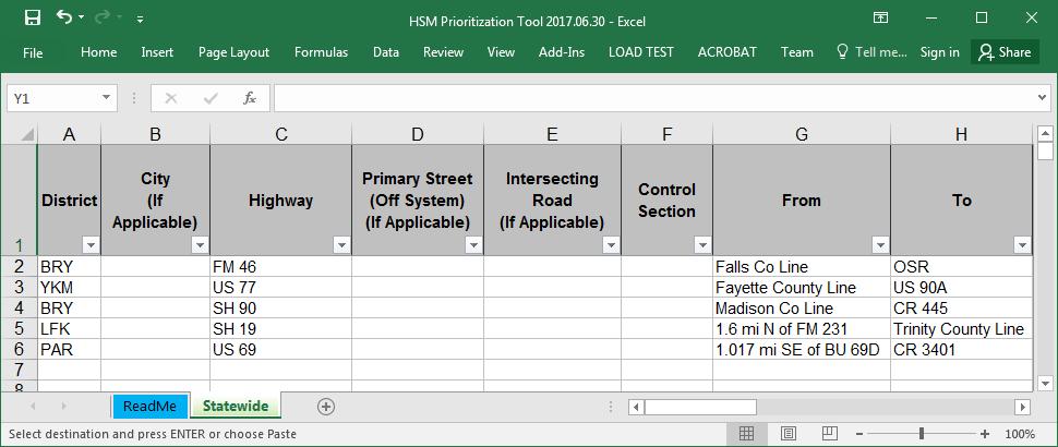
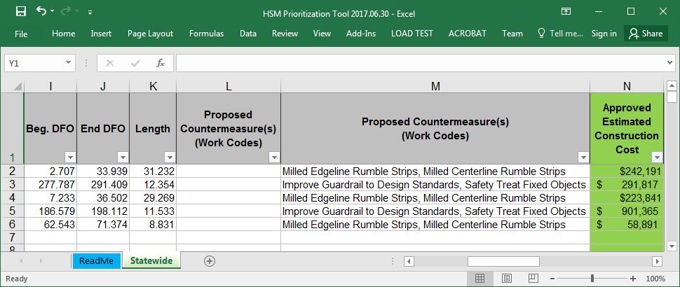
137 Figure 42. Screenshots of Project Prioritization Tool. 121