AN INTEGRATED GROUNDWATER RECHARGE AND FLOW MODEL TO PREDICT BASE FLOW

Transcription

1 AN INTEGRATED GROUNDWATER RECHARGE AND FLOW MODEL TO PREDICT BASE FLOW By XIAOJING NI A THESIS Submitted to Michigan State University in partial fulfillment of the requirements for the degree of Civil Engineering - Master of Science 2014

2 ABSTRACT AN INTEGRATED GROUNDWATER RECHARGE AND FLOW MODEL TO PREDICT BASE FLOW By Xiaojing Ni As with many environmental processes groundwater recharge and stream base flow are complex and not completely understood. The study involved the coupling of an unsteady recharge model and groundwater model to a 150 km 2 watershed in Michigan s Hillsdale and Branch Counties that is drained by a groundwater-dependent stream. The study utilized existing statewide databases with detailed data on land use and cover, soils and root zone depth, climate, glacial and bedrock geology and associated hydraulic conductivity, digital elevation model, and stream and lake topography and topology. Annual base flow in the stream was shown to be significantly smaller than annual recharge primarily due to potentially significant surface seepage from streams to wetlands and lakes. Despite the seasonal variability of recharge, the variability in the base flow was less than expected because of the buffer effect of the aquifer. This buffer effect results in winter base flows being significantly lower than expected (based on classically expected recharge rates) and summer base flows being significantly higher than expected. This situation in which predicted summer base flows are higher than measured stream flows is potentially due to significant surface water evaporation and near-stream saturated soil evapotranspiration.

3 TABLE OF CONTENTS LIST OF TABLES... v LIST OF FIGURES... vi LITERATURE REVIEW... 3 OBJECTIVE... 5 APPROACH... 6 Watershed Model... 6 Canopy interception... 8 Snowpack... 9 Net infiltration Initial capacity of soil Drainage and redistribution of water in soil profiles Evapotranspiration Recharge Transient Coupled Recharge and Groundwater Model Groundwater head Base flow APPLICATION Description of the Study Area Input Data Digital elevation model and bedrock elevation Hydraulic conductivity Topsoil type Land use and cover Other input Conceptual model Calibration Results and Discussion Results of calibration Results of groundwater head iii

4 Results of annually recharge Results of Monthly Recharge CONCLUSIONS APPENDIX REFERENCES iv

5 LIST OF TABLES Table 1. Soil type parameters Table 2. Land use and cover parameters v

6 LIST OF FIGURES Figure 1. Modeling System... 6 Figure 2. Study Area Figure 3. Digital Elevation Model Figure 4. Cross Sections of Study Area Figure 5. Hydraulic Conductivity Figure 6. Clay Distribution Figure 7. Land Use and Cover Figure 8. Conceptual Model Figure 9.Average Seepage Area Figure 10. Direct Base Flow and Total Base Flow Figure 11. Base Flow and Seepage Figure 12. Base Flow and Recharge Figure 13. Recharge and Base Flow in Regular Scale Figure 14. Storage Release in Summer Figure 15. Statewide Well Data Calibration Figure 16. Groundwater Head vi

7 Figure 17. Distribution of Annual Recharge Figure 18. Monthly Recharge vii

8 INTRODUCTION Groundwater is a critical source of stream, since it can influence stream temperature and provide a suitable year-round habitat for fish (Barlow and Leake, 2012). The State of Michigan limits large quantity groundwater withdrawals to a fraction of the stream index flow, which is defined as the 50 percent exceedance (median) flow during the summer months of the flow regime (Hamilton et al.,2008). Implementing / complying with the State s limits requires knowing the base flow in the streams, especially during the summer. In the summer, evaporation rates and plant growth/transpiration rates increase, so that the water level / flow in the stream is at its lowest annual level, which will affect fish in the stream. Most of flow in stream is base flow from groundwater in summer. The current approach to predicting base flow involves direct stream flow measurements where USGS gaging stations are available. However, most streams of interest especially smaller headwater streams have no nearby USGS gaging station. In these cases, prediction of base flow is based on the use of a statewide regression model based on USGS gaging station base flow measurements indexed based on watershed area. Preliminary analyses of the accuracy of this regression model show that the predicted base flow has significant errors, especially for small streams. These small streams are extremely important for groundwater dependent ecosystems. This research focuses on predicting base flow both spatially and temporally through the 1

9 use of several grid-based models. The fundamental technical approach involves using a process-based simulation approach to calculate base flow. In the study discussed throughout this paper, a watershed model using forty years of climate records was developed and used to predict annual average recharge and average moisture conditions in the soil. The predicted groundwater level was used for calibration. Finally, a transient watershed model coupled with a groundwater model was constructed and used to calibrate the watershed model against ten-years worth of stream flow measurements. 2

10 LITERATURE REVIEW Based on the measurements of stream flow, base flow recession analysis gives analytical solution of base flow based on theoretical equation of groundwater flow which is derived from the Boussinesq equation. The use of the base flow recession model was based on the assumption that the aquifer is a Depuit-Boussinesq -type aquifer (Hall, 1968). This model shows that the relationship of logarithmic base flow and time is linear during the summer. Based on their base flow recession study, an automated method for the estimation of base flow was introduced by Arnorld and Allen (1999). They used the digital filter with empirical parameters (without physical basis) to extract surface runoff values from stream flow. The statistical method which is used by USGS (Hamilton et al., 2008) for implementing this approach is to predict total stream flow using a regression model based on many hydrologic characteristics including: percentage of the basin where land cover is classified as forest; precipitation in inches; and numerous other parameters. The regression model has the ability to predict index flow on a large scale. The chosen characteristics, which are used to derive the regression model, are not supported by physical reality. The regression model has an inherent failure to deal with the influence-points problem in statistics. As such, large stream flows will greatly impact the slope of the linear regression and thus negatively affect the overall performance of the 3

11 regression model. Because of these problems, errors can range from 0.059% to 529%. According to 2008 Michigan Legislation, the largest cumulative percentage reduction in stream index flow allowed is 25%. The large-capacity withdrawal of ft 3 /s (Hamilton and Seelbach, 2010) would cause an adverse impact with the average index flow of the stream being ft 3 /s. If the error is 200%, the index flow would be ft 3 /s, and the withdrawal limit would be ft 3 /s, which means that all the water in the stream would be withdrawn by pumping. 4

12 OBJECTIVE The objective of the research was to investigate the use of a process-based numerical model as an alternative to estimating base flow in small watersheds. The spatial and temporal variations in base flow produced by the process-based and traditional approaches are presented and discussed as the basis for evaluation. Additionally, any other characteristics of the relationship between recharge and base flow that are illuminated by the investigation are also discussed. 5

13 APPROACH The basic approach involved integrated recharge and groundwater modeling. The approach consisted of three steps: 1) calculating annual recharge and average soil saturated condition in the watershed model. Interception, snowpack, evapotranspiration, runoff and percolation were taken into account in the watershed model; 2) constructing a groundwater model which was then used for simulating groundwater flow; and 3) developing a transient coupled recharge and groundwater model, which was used to calibrate both the watershed model and the groundwater model. This modeled base flow was then compared with available stream base flow measurements. Figure 1. Modeling System Watershed Model A distributed parameter watershed model was used to estimate the recharge to 6

14 groundwater. The watershed model used a rectangular grid-base model to solve the water balance equations. The Environmental Protection Agency (EPA) defines a watershed as the area of land where all of the water that is under it or drains off of it goes into the same place. The physical process of water flowing through the watershed can be summarized through the following cycle: 1) water falls towards earth through precipitation; 2) some of this water is physically intercepted by vegetation; 3) the water that reaches the ground either flows over land or seeps into the ground; 4) as water seeps through the root zone, some of it will be taken by plant roots dues; 5) the intercepted and taken-up water will return to the atmosphere through evapotranspiration; 6) water will also evaporate from the topsoil layer under the right conditions. Seasonal conditions will impact this process, the most drastic example being that of precipitation in the form of snow being stored on land and later running off in great quantities when the temperature rises. All important seasonal variability has been taken into account. The water balance equation used to calculate net infiltration is NI = PRCP-Interception+Qin-ET-Qout-S (1) Where NI is net infiltration PRCP is precipitation including rainfall and water from snow melt Interception is water intercepted by vegetation canopy 7

15 Q in is water from adjacent cells Q out is water to adjacent cells ET S is potential evaporation from soil and evapotranspiration from vegetation is storage in soil To estimate recharge, IGW uses a method based on INFIL model to calculate daily recharge. The rectangular grid-base model uses DEM, daily precipitation, daily temperature, soil type, vegetation and root zone depth as its input. These inputs are distributed across the grid s cells. When using the water balance approach to calculate the recharge of each cell, the model uses the particular input of each cell. Canopy interception In a given area, the actual amount of rainfall that reaches the ground is reduced by physical interception. The intercepted water evaporates over time, and thus the actual interception capacity changes over time, ranging from its maximum capacity to zero, depending on when the following precipitation event occurs. A simple estimation of canopy interception is Water falls onto ground={ (2) Where P is precipitation, in mm 8

16 a is interception of vegetation canopy, in mm R is amount of water falling onto ground a is interception capacity after precipitation Snowpack Snowfall affects the magnitude and distribution of recharge, and will thus affect the infiltration capacity of soil. When snow is accumulating, precipitation does not easily infiltrate into the soil. IGW uses the method in SWB (Westenbroek al et. 2010) to define snow pack temperature as ( ) (3) Where T SG is snow pack temperature, C T max is maximum temperature of a day, C T min is minimum temperature of a day, C The snow pack temperature is a function of the maximum temperature and minimum temperature during the preceding days. And when snow pack occurs, infiltration capacity of soil is reduced to one third of original capacity. The SWAT method (Neitsch, 2000) is used to estimate snow melting as a function of 9

17 maximum temperature and snowpack temperature, specifically Where SNO mlt is the amount of snow melt on a given day, mm [ ] (4) b mlt is the melt factor for the day, mm /(day* C) sno cov is the depth of snow covering the cell, mm T SG is the snow pack temperature on a given day, C T max is the maximum air temperature on a give day, C T mlt is the base temperature above which snow melt is allowed, C Seasonal variation is considered when estimating melt factor. ( ) ( ( )) (5) Where b mlt6 is the melt factor for June 21, mm/(day* C) b mlt12 is the melt factor for December 21, mm/(day* C) d n is the day number of the year Net infiltration Hortonian runoff processes and Dunnian runoff processes are used to describe infiltration and runoff. There are four primary steps when simulating runoff for each cell in a model 10

18 grid. The first step is calculating the initial infiltration capacity of soil. Any excess water causes a Hortonian runoff process. The second step is redistributing the infiltration in the root zone and estimating the storage in the soil. The third step is the calculation of evapotranspiration. The fourth step is estimating the net infiltration and Dunnian runoff due to the saturation of soil. 1. Initial capacity of soil In IGW, the seasonal infiltration capacity, or maximum rate at which water can infiltrate into the soil, is calculated based on the initial capacity of the soil as represented by (6) Where IC is the infiltration capacity K sat is saturated vertical hydraulic conductivity, m/day T is event occurring duration (default = 12, summer = 2, winter = 4, snow melt =8), hours If the intensity of rainfall and snowmelt are less than IC, then soil still has capacity to take water. Otherwise, the water flows into a downstream cell as runoff. 2. Drainage and redistribution of water in soil profiles A modified gravity-drained rectangle model introduced by Jury et al. (1991) is used to 11

19 estimate the movement of water down through the six layers in the root zone soil profile. It is formulated as ( ) (8) Where D j is drainage through layer j into layer j+1 in a particular cell is initial volumetric water content is final volumetric water content d is thickness of layer j ( ) (9) ( ) (10) ( ) (11) ( ) (12) (13) Where n is porosity of the soil is 2*n+3, a constant for particular soil is time step 12

20 is simulated water content 3. Evapotranspiration Evapotranspiration where water evaporates/transpires from the soil and from plants before it infiltrates into deeper soil layers has two functional components: potential evapotranspiration and plant evapotranspiration. The mechanics of these two processes are discussed separately. 1) Potential Evapotranspiration A modified Priestley-Taylor equation (Davies and Allen, 1973; Flint and Childs, 1991) is used to estimate potential evapotranspiration in bare soil. Potential evaporation is assumed to occur in first two layers (USGS, 2008) as given by ( ) (14) Where PET is potential evapotranspiration is modified Priestley Taylor coefficient s is slope of the saturation vapor density curve is the psychrometric constant R n is radiation G is soil heat flux 13

21 α' is a function of water content of soil, which is defined as following equations. ( ) ( ) (15) Where are bare-soil coefficients is relative saturation at cell i and layer j is vegetation cover for cell i (16) Where is the water content of soil is porosity is the residual soil-water content 2) Evapotranspiration from plant roots A modified Priestley-Taylor equation was used to simulate this process. Similar to the modified Priestley-Taylor equation used to describe potential evapotranspiration, is used instead of, in this Priestley-Taylor equation and is given as { [ ( ) ]} (17) Where W is weighting factor 14

22 is soil-transpiration coefficient is relative saturation at cell i and layer j is vegetation cover for cell i ( ) (18) Where is relative saturation at cell i for layer j is root density factor at cell I for layer j 4. Recharge Based on the previous three steps, recharge to the groundwater is equal to the net infiltration. After storage, drainage, and evapotranspiration are considered, the remaining water enters deep soil where hydraulic conductivity controls the percolation into the water table through (USGS, 2008) { (19) Where NI is net infiltration K s is saturated hydraulic conductivity of deep soil D is drainage is water content of deep soil 15

23 SC is storage capacity of deep soil K is unsaturated hydraulic conductivity of deep soil Transient Coupled Recharge and Groundwater Model A two-dimensional transient groundwater model with transient recharge from the watershed model was applied to calibrate both the watershed and groundwater models. Other data used to develop the groundwater model includes topographic elevations, bedrock elevations, and hydraulic conductivity from the statewide groundwater database. calculated by the watershed model is the initial condition of the soil in the transient groundwater model. Base flow is defined as the component of stream flow that is derived from groundwater, and it is controlled by both groundwater head and surface water head. In this model, a digital elevation model (DEM) was used to simulate the head in the river. Recharge has a direct impact on the groundwater head, which in turn determines relative to stream head if groundwater flows into a stream as base flow (which it does if it is greater than stream head). Groundwater head The daily recharge calculated by the watershed model is an input into the groundwater model ( ). The transient water balance based on Darcy s law is calculated to simulate 16

24 the amount of water flow into a stream from groundwater as represented by [( ) ] [( ) ] (20) Where h is hydraulic head is bottom elevation of aquifer and are hydraulic conductivity in x and y directions, respectively is storativity is sources and sinks at time t (21) Where is recharge at time t, is leakage from river or lake at time t is pumping from aquifer at time t is base flow at time t D is drainage to surface a, b, c, d and e are 1 or 0. If the source or sink term occurs, they equal 1. Otherwise, they equal 0. Base flow 17

25 Base flow is the portion of groundwater that flows into a stream. We can predict base flow by calculating the water balance of groundwater after the groundwater table level is elevation is determined. In order to solve for the groundwater table elevation, Equation 20 is dissolved using a finite difference method. After solving for the groundwater table elevation, then accounts for all sources and sinks of groundwater for grid i and equation 21 is modified to show this as (22) Where is recharge at grid i is leakage from river or lake at grid i is pumping from aquifer at grid i is base flow is surface water drainage a, b, c, d and e are 1 or 0. If the source or sink term occurs, they equal 1. Otherwise, they equal 0. When Where K d is leakance of surface 18

26 A i is area of cell Leakage (L i ) is a function of head difference between the lake/river level and groundwater level as defined as (23) Where A i is area of cell is leakance of river or lake is hydraulic head of river or lake in the grid h i is hydraulic head of groundwater at the grid 19

27 APPLICATION Description of the Study Area The representative small area watershed is between Hillsdale County and Branch County, MI. The area consists of two sub-watersheds with area about 150 km 2. There are second and third order streams and fifth and fourth order lakes in this area. The aquifer in this area is thin due to bedrock elevation is high. A stream flow gaging station is placed in the outlet of the watershed. The result of recharge from regression model used by USGS shows the recharge is high in and along the rivers. Input Data Input data include Digital Elevation Model (DEM), bedrock elevation, topsoil type, land use, land cover, hydraulic conductivity, precipitation and temperature. 20

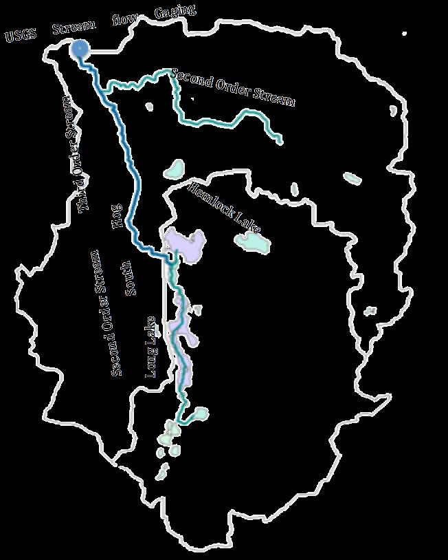
28 Figure 2. Study Area 21

29 Digital elevation model and bedrock elevation The digital elevation model is a representation of topography. In the watershed model, the 30 m resolution DEM was used to estimate overland flow direction. And in the groundwater model, the DEM defines the aquifer top for the model groundwater level. Figure 3 is the DEM model. The thickness of the glacial layer is variable in this watershed. According to well data, the depth to the bedrock can reach up to 60 ft. 22

30 Figure 3. Digital Elevation Model Hydraulic conductivity 23

31 Hydraulic conductivity of the glacial layer is also calculated from the well data. And the hydraulic conductivity of bedrock, which is Coldwater shale in this area, is defined as 5 ft/day, - a typical value of fractured rock hydraulic conductivity (El-Naqa, 2000). The weighted arithmetic mean of hydraulic conductivities of the two layers is considered as the hydraulic conductivity of the modeled layer. Cross section Figure 4. Figure Cross 4. Sections Cross sections of Study Area 24

32 Figure 5. Hydraulic Conductivity Topsoil type Topsoil type affects potential evaporation and percolation. Different soil has different properties, such as saturated hydraulic conductivity and water content. According to percentage of clay, sand and silt, 12 classifications used by Soil Texture are determined to 25

33 describe all kinds of soil. The topsoil type data is from SSURGO database. Some missing area is set as default soil texture value by different properties. For river well connected with aquifer, recharge is not taken into account as net infiltration to groundwater. And for lake, the bottom is covered by less permeable material to prevent water infiltrated. So lake and river bottom are defined as less permeable area using soil texture of 70% clay, 10%sand and 20%silt. Some permeable missing area such as beaches is set as default permeable soil texture of 5% clay, 80% sand and 15% silt. Figure 6 shows the clay distribution through the whole area. Land use and cover According to NLCD Land Cover Class Definition, land use and cover is divided into 20 classifications including barren land, deciduous forest, evergreen forest, shrub and grassland etc. 26

34 Figure 6. Clay Distribution 27

35 Figure 7. Land Use and Cover Other input 28

36 The climate station is in Branch County about 15 kilometer away from the stream outlet. When using the watershed model to estimate annual recharge, daily precipitation and maximum and minimum temperature records for 40 years ( ) from the Global Historical Climatology Network-Daily Database (GHCN-D) were used. Ten year ( ) records were used in the transient groundwater model. Missing data was set as a default value which is the daily average precipitation for each year. The hydraulic conductivity used in the model was interpolated from well data. Conceptual model The following considerations were utilized in developing the conceptual model: Evapotranspiration and snowpack were considered in the watershed model. Pumping was not taken into account for this site. The watershed boundary was defined as a no flow boundary for both surface water and groundwater. Streams were modeled in such a way that water only flows into them. Small streams do not supply water during the summer. All lakes were considered as seepage sources. In order to solve differential equations, a finite difference method was used. 29

37 Watershed no flow boundary In the watershed model for estimating annual recharge, the time step is one day. The resolution of the model is 116*121m. There are two different ways to model streams: two way, which means the water can flow from and to the stream this method affects the slope of the base flow one way, which means the water can only flow into the stream from the aquifer. Precipitation Evapotranspiration 2-D Conceptual Model Snowpack One-way stream Recharge Groundwater flow Base flow Seepage One layer Coldwater shall - no flow boundary Figure 8. Conceptual Model Calibration Water level from the steady state groundwater model was compared with data from the statewide well database to calibrate groundwater parameters such as hydraulic 30

38 conductivity and aquifer thickness. There are 63 wells in this watershed. A transient model coupled to the groundwater model was used to calibrate the watershed model. To estimate initial condition of groundwater, a 13 year time series was used to simulate average conditions of groundwater. And ten years of results were used to calibrate the model. Base flow calculated in the transient groundwater model with transient recharge from watershed model was compared with stream flow records from the USGS stream flow gaging station to calibrate base flow. Results and Discussion Results of calibration A water budget analysis was performed to compute stream base flow. Drain leakance was defined as 0.01/day. When the streams are considered as a polyline, the magnitude of base flow is very sensitive to surface drain rate. Drain leakance is adjusted from 1 1/day to /day, which caused the magnitude of base flow to ranges from 10 2 to 10 5 m 3 /day. According to seepage area in Figure 9, which shows seepage occures along the stream where elevation is low, seepage should be considered as base flow. 31

39 Figure 9.Average Seepage Area 32

40 The leakance is 10 m/day for third order stream and 0.5 m/day for second order stream. Leakance changed from 1 to 500 for third order, but the magnitude of the base flow is the same. Figure 10 shows a comparison of the direct base flow and total base flow. In log scale, the slope of direct and total base flow in summer is the same. When the stream is treated as a polyline, direct base flow is the water directly flowing into the stream in a river cell. But water seeped to ground over wetland areas around the stream does not evaporate directly. Some of the seeped water flows into the streams due to low elevation. Figure 11 shows recharge and seepage over the whole modeled area and base flow directly into the streams. Long-term recharge is equal to the sum of base flow and water drained to surface. Water drained to the surface is defined as when the calculated groundwater head is higher than DEM. In this case water flows onto the ground and evaporates directly. 33

41 Discharge, cfs Precipitation, inch/day Precipitation Stream Flow Direct Base Flow Total Base Flow Figure 10. Direct Base Flow and Total Base Flow 34

42 1/1/03 3/7/03 5/11/03 7/15/03 9/18/03 11/22/03 1/26/04 3/31/04 6/4/04 8/8/04 10/12/04 12/16/04 2/19/05 4/25/05 6/29/05 9/2/05 11/6/05 1/10/06 3/16/06 5/20/06 7/24/06 9/27/06 12/1/06 2/4/07 4/10/07 6/14/07 8/18/07 10/22/07 12/26/07 2/29/08 5/4/08 7/8/08 9/11/08 11/15/08 1/19/09 3/25/09 5/29/09 8/2/09 10/6/09 12/10/09 2/13/10 4/19/10 6/23/10 8/27/10 10/31/10 1/4/11 3/10/11 5/14/11 7/18/11 9/21/11 11/25/11 Discharge, cfs Precipitation, inch/day Precipitation Baseflow and Seepage within whole area Recharge Figure 11. Base Flow and Seepage 35

43 Focusing on one of the simulated years, figure 12 shows the results of calibration. From calibration results, the calibration can catch the trend of change of base flow, but not runoff into stream. In spring, recharge is highest dues to plenty of water infiltrated into aquifer dues to snow melting. The recharge and base flow are high when precipitation is high. Recharge is higher than base flow in spring, because water was stored in aquifer. In summer, base flow is higher than recharge dues to that water is released from storage in the aquifer. The predicted base flow in summer is higher than base flow in summer. One guess of this is evaporation in the stream is not taken into account. The evaporation from dry stream bed can be up to 0.55 mm/day during dry summer (Fox, 1968). Thus, evaporation from stream can be a significant part of the discharge in stream. Also, the stream is modeled as constant head. In winter, elevation of stream should higher than modeled, where surface water drain should be taken into account. But in summer, stream elevation is low and evaporation rate is high, so that most of surface water drain evaparate directly. 36

44 Discharge, cfs Precipitation, inch/day /1/06 2/1/06 3/1/06 4/1/06 5/1/06 6/1/06 7/1/06 8/1/06 9/1/06 10/1/06 11/1/06 12/1/06 1/1/07 Precipitation Stream Flow Recharge Total Base Flow Figure 12. Base Flow and Recharge 37

45 1/1/03 3/14/03 5/25/03 8/5/03 10/16/03 12/27/03 3/8/04 5/19/04 7/30/04 10/10/04 12/21/04 3/3/05 5/14/05 7/25/05 10/5/05 12/16/05 2/26/06 5/9/06 7/20/06 9/30/06 12/11/06 2/21/07 5/4/07 7/15/07 9/25/07 12/6/07 2/16/08 4/28/08 7/9/08 9/19/08 11/30/08 2/10/09 4/23/09 7/4/09 9/14/09 11/25/09 2/5/10 4/18/10 6/29/10 9/9/10 11/20/10 1/31/11 4/13/11 6/24/11 9/4/11 11/15/11 1/26/12 4/7/12 6/18/12 8/29/12 11/9/12 Discharge, cfs Precipitation, inch/day Precipitation Recharge Total Base Flow Figure 13. Recharge and Base Flow in Regular Scale 38

46 Discharge, cfs Precipitation, inch/day Figure 13 shows relationship of recharge and total base flow in regular scale. From 2003 to 2012, average of recharge is cfs for whole study area. Average base flow in summer is 8.39 cfs. The difference between recharge and base flow is surface water drain including lake area. Figure 14 shows how the different specific yield affects the slope of storage releasing. Recharge in summer is set as zero by limiting the infiltration initial capacity of soil, so that the storage releasing should be linear to time in semi-log scale. Storage releasing Precipitation Stream flow Sy=0.05 Sy= /1/2008 5/1/2008 6/1/2008 7/1/2008 8/1/ Figure 14. Storage Release in Summer Groundwater model calibration (Figure 15) was performed utilizing static water level data available from the domestic water well records. Hydraulic conductivity is 30% of weighted arithmetic mean hydraulic conductivity. Specific yield is 0.01 and Storage coefficient is 1.0E-7. The figures below show the simulated static water levels and base flow. The water level compared with data from statewide well data shows most of points are in the confidential interval of one standard deviation. The RMS error is 4.32 and 39

47 mean error is The reason why some of modeled head are closed to 310ft which are different from data is that stream level is modeled as constant based on DEM. Figure 15. Statewide Well Data Calibration Results of groundwater head Figure 16 shows the groundwater head at the site. Water from the boundary of the watershed flows into the stream. 40

48 Figure 16. Groundwater Head Results of annually recharge Recharge in this area is shown below. Locations with small K s have small recharge. The high value appears beside the lake. Because the cells in lake area are set as less permeable and the cell beside the lake is sandy loam which is permeable material, water flows into cells with low DEM, the lake area, and infiltrate into ground in cells with permeable 41

49 material. Figure 17. Distribution of Annual Recharge Results of Monthly Recharge The figure below shows average monthly precipitation, modeled actual evapotranspiration and modeled recharge for one selected point. Precipitation of this area has little seasonal change. Average monthly recharge is low in summer due to high 42

50 Inch of water per year evapotranspiration. Average recharge is lowest in summer and evaporation is highest due to high temperature. The highest recharge occurs in March when the temperature increases and snow starts to melt Recharge Precipitation Potential Evapotranspiration Actual Evapotranspiration 0 Jan Feb Mar Apr May Jun Jul Aug Sep Oct Nov Dec Figure 18. Monthly Recharge 43

51 CONCLUSIONS The simulation and model sensitivity analysis illuminate numerous interesting characteristics of this particular watershed/stream/groundwater system. Expectedly, the results show that recharge exhibits extreme spatial variability due primarily to local soil variability. The recharge is also shown to be significantly seasonally variable, with highest levels in the spring due in large part to thawing and snow melt and lowest levels in the summer due to high evapotranspiration. Annual base flow in the stream was shown to be significantly smaller than annual recharge even without considering any groundwater withdrawals (i.e. pumping) primarily due to potentially significant surface seepage from streams to wetlands and lakes. Despite the seasonal variability of recharge, the predicted variability in the base flow is less than expected primarily because of the buffer effect of the aquifer. This buffer effect results in predicted winter base flows being significantly lower than expected (based on classically expected recharge rates) and predicted summer base flows being significantly higher than expected. This situation in which predicted summer base flows are higher than measured stream flows is potentially due to significant surface water evaporation and near-stream saturated soil evapotranspiration. 44

52 FUTURE WORK The model did not perform well in summer. Evaporation in the stream needs to be considered. And drainage area measurement or more research on modeling seepage is needed in the future. Additional research is also needed for the quantity of water from seepage that should be included in base flow. Future work should also include calculating the index flow and comparing with regression method. 45

53 APPENDIX 46

54 APPENDIX Class Table 1. Soil type parameters Root Root Root Root Root Root Root Root Root Root Index Intercept Canopy Depth Depth Depth Depth Depth Density 1 Density 2 Density Density Density Class Name Manning ion(mm) Cover(%) (%) (%) 3(%) 4(%) 5(%) Open Water Perennial Ice/Snow Developed/Open Space Developed/Low Intensity Developed/Medium Intensity Developed/High Intensity Barren Land(Rock/Sand/Clay) Deciduous Forest Evergreen Forest Mixed Forest Dwarf Scrub Shrub/Scrub Grassland/Herbaceous Sedge/Herbaceous Lichens

55 Table 1 (cont d) Moss Pasture/Hay Cultivated Crops Woody Wetlands Emergent Herbaceous Wetlands

56 Table 2. Land use and cover parameters Class Name Ks (cm/h) Hav(cm) θs θr θ0 θc λ Sand Loamy sand Sandy loam Loam Silt loam Silt Sandy clay loam Clay loam Silty clay loam Sandy clay Silty clay Clay

57 REFERENCES 50

58 REFERENCES Arnold, J. G., Allen, P. M., Muttiah, R. and Bernhardt, G. (1995), Automated Base Flow Separation and Recession Analysis Techniques. Groundwater, 33: doi: /j tb00046.x Barlow, P.M., and Leake, S.A., 2012, Streamflow depletion by wells Understanding and managing the effects of groundwater pumping on streamflow: U.S. Geological Survey Circular 1376, 84 p. (Also available at ) Davies, J.A., and Allen, C.D., 1973, Equilibrium, potential and actual evaporation from cropped surfaces in southern Ontario: Journal of Applied Meteorology, v. 12, p El-Naqa, A. (2000) The hydraulic conductivity of the fractures intersecting Cambrian sandstone rock masses, central Jordan, Environmental Geology 40: Flint, A.L., and Childs, S.W., 1991, Use of the Priestley-Taylor evaporation equation for soil water limited conditions in a small forest clearcut: Agricultural and Forest Meteorology, v. 56, p Fox, Michael J., 1968: A Technique to Determine Evaporation from Dry Stream Beds. J. Appl. Meteor., 7, Gupta, Ram S.. "Horton's Infiltration Model." Hydrology and hydraulic systems. 2nd ed. Prospect Heights, Ill.: Waveland Press, Print. Hamilton, D.A., Sorrell, R.C., and Holtschlag, D.J., 2008, A regression model for computing index flows describing the median flow for the summer month of lowest flow in Michigan: U.S. Geological Survey Scientific Investigations Report , 43 p. Date Posted: August 1, 2008: available only at [ Hall, F.R., Base flow recessions--a review. Water Resour. Res., 4(5): Hamilton, D. A. and Seelbach, P. W Determining environmental limits to streamflow depletion across Michigan, volume 42. In The book of the states, 2010 edition, Edited by: Wall, A. S Lexington,, Kentucky: The Council of State Governments. Jury, W.A., Gardner, W.R., and Gardner, W.H., 1991, Soil physics (5th ed.): New York, John Wiley and Sons, 328 p. 51

59 Neitsch, S.L., Arnold, J.G., Kiniry, J.R., and Williams, J.R., 2002, Soil and Water Assessment Tool Theoretical Docu- mentation, version 2000: Temple, Texas, Grassland, Soil and Water Research Laboratory, Agricultural Research Service. U.S. Geological Survey, 2008, Documentation of computer program INFIL3.0 A distributed-parameter watershed model to estimate net infiltration below the root zone: U.S. Geological Survey Scientific Investigations Report , 98 p. ONLINE ONLY Westenbroek, S.M., Kelson, V.A., Dripps, W.R., Hunt, R.J., and Bradbury,K.R., 2010, SWB A modified Thornthwaite-Mather Soil-Water-Balance code for estimating groundwater recharge: U.S. Geological Survey Techniques and Methods 6 A31, 60 p. 52